The Shannon Sampling Theorem states that if a signal f(t) contains no frequencies greater than W. 2 cycles per second, then the signal is completely determined ...
Using the Shannon Sampling Theorem to Design Compact Discs Susan E. Kelly Abstract The Shannon Sampling Theorem states that if a signal f (t) contains no frequencies greater than W 2 cycles per second, then the signal is 1 completely determined by its values at a sequence of points spaced W seconds apart. Using this theory, music can be stored on a compact disc by recording the function’s amplitude at points sampled at the correct rate. This material, including the proof provided for the theorem, is accessible to students who have done some work with Fourier series and transforms. With modifications, the same ideas could be given to Calculus students to illustrate the usefulness of series. The author has used this material with students at both of these levels.
Have you ever wondered how music is stored on a compact disc and then reproduced? Mathematically the music can be viewed as a function in time. To record the music on a disc, the function is converted to a series of numbers which represent the function’s amplitude at evenly spaced points in time. These numbers are what are stored on the disc. The Shannon Sampling Theorem explains how many amplitude readings are needed and how these numbers are used as the coefficients of a series which will reproduce the music. To understand this theorem, it is necessary to examine a small amount of Complex Number theory and some Fourier Analysis. The Shannon Sampling Theorem will then be given and we will see how it can be applied to the design of compact discs and players.
1
Background in Complex Numbers
A few basic facts from Complex numbers are needed. In this theory i is defined as the square root of -1. The complex numbers are defined to be 1
the collection of all elements of the form z = x + iy, where x and y are real numbers. In Calculus courses several series representations for real valued functions are studied. For example, ex = 1 +
x x2 x3 + + + ... , 1! 2! 3!
sin x = x −
x3 x5 + − ... , 3! 5!
and
x2 x4 + − ... . 2! 4! These series converge absolutely and uniformly if x lies in any finite interval. These formulae can be extended to complex valued functions of a complex variable. For example, cos x = 1 −
ez = 1 +
z2 z3 z + + + ... 1! 2! 3!
.
It can be shown that the above series is uniformly convergent if |z| ≤ N , for each N > 0. Letting z = ix, where x is a real number, yields Euler’s formula, eix = cos x + i sin x.
(1)
From this it is easy to show that cos(x) =
eix + e−ix 2
(2)
and
eix − e−ix . (3) 2i These last three formulas are all that we shall need from Complex numbers. sin(x) =
2
Fourier Analysis
Some background in Fourier Analysis is also needed. A Fourier sine and nt nt ∞ cosine series is based on the fact that the set { √12 , cos( W ), sin( W )}n=1 is an
2
orthogonal set in the interval [−πW, πW ]. That is, for elements g1 and g2 of the set, ( Z πW 0 if g1 6= g2 g1 (t)g2 (t)dt = (4) πW if g1 = g2 . −πW This can be verified using several cases. The work can be simplified using properties of even and odd functions and the complex exponential representations of sine and cosine functions given in Equations (2) and (3). With this result we wish to represent a 2πW -periodic function in terms of a sine and cosine series, ∞ X 1 nt nt f (t) = a0 + [an cos( ) + bn sin( )]. 2 W W n=1
(5)
If this series is valid, all that is needed are the values for the coefficients. For nt ) and example, to solve for an , multiply both sides of Equation (5) by cos( W integrate. (This process uses term-by-term integration which requires special convergence conditions on the series. For example, uniform convergence would be sufficient. We will not deal with the convergence issue in this paper.) After changing the index on the summation, Z πW −πW
f (t) cos(
nt )dt = W
1 a0 2 +
Z πW −πW
∞ X
[am
cos(
nt )dt W
Z πW
m=1
+bm
−πW
cos(
Z πW −πW
nt mt ) cos( )dt W W
sin(
nt mt ) cos( )dt]. W W
By property (4), all terms drop out of the right hand side except for the an term, Z πW nt f (t) cos( )dt = an πW. W −πW Thus, Z πW 1 nt an = f (t) cos( )dt. πW −πW W With similar work the bn coefficients can be found. A 2πW -periodic function f (t) can now be represented by an infinite series. The sine and cosine form of the Fourier Series for f (t) is ∞ X nt nt 1 [an cos( ) + bn sin( )]. f (t) ∼ a0 + 2 W W n=1
3
(6)
where the Fourier coefficients are defined to be Z
πW nt 1 f (t) cos( )dt πW −πW W Z πW 1 nt = f (t) sin( )dt πW −πW W
an =
for n = 0, 1, 2, ...
bn
for n = 1, 2, ...
Dirichlet’s Theorem states that if a function has a finiteRnumber of extrema πW and discontinuities on the interval [−πW, πW ] and if −πW |f (t)|dt < ∞, then the Fourier series in (6) converges to f(t) at all points where the function is continuous. The series converges to the midpoint of the jumps at points of discontinuity. This pointwise convergence result is what is meant by the ∼ symbol used in Equation (6). Similar work can be done with the orthogonal set {eint/W }n∈Z . The complex exponential form of the Fourier series for a 2πW -periodic function is ∞ X
f (t) ∼
cn eint/W ,
(7)
n=−∞
where
1 2πW
cn =
Z πW −πW
f (t)e−int/W dt.
Note that this series could also represent a nonperiodic function on the interval [−πW, πW ]. This last idea can be extended to piecewise smooth L1 (R) function, R∞ −∞ |f (t)|dt < ∞. The following approach illustrates the idea, but is not rigorous. A formal proof would require additional conditions on the function. Define fW to be the 2πW -periodic function equal to f on (−πW, πW ). Then from Equation (7) fW (t) ∼
∞ X
(
n=−∞
Z πW
1 2πW
−πW
f (x)e−inx/W dx)eint/W .
Letting ξn = n/W and ∆ξn = ξn+1 − ξn = 1/W , ∞ X
1 fW (t) ∼ ( 2πW n=−∞ ∞ X
1 ( = 2π n=−∞
Z πW −πW
Z πW −πW
f (x)e−iξn x dx)eiξn t W ∆ξn
f (x)e−iξn x dx)eiξn t ∆ξn .
4
Now, as W → ∞, fW → f and 1 f (t) ∼ √ 2π
Z ∞
1 (√ 2π −∞
Z ∞ −∞
f (x)e−iξx dx)eiξt dξ.
This motivates the definition for the Fourier transform. Definition 2.1 For f ∈ L1 (R), the Fourier transform of f is 1 fˆ(ξ) = √ 2π
Z ∞ −∞
f (t)e−iξt dt
and the inverse Fourier transform is 1 fˇ(t) = √ 2π
Z ∞ −∞
f (ξ)eiξt dξ.
We can think of f (t) as a function in the time domain and fˆ(ξ) as the functions frequency content. The Fourier Inverse Theorem states that if f and fˆ are in L1 (R), then (fˆ)ˇ= (fˇ)ˆ= f almost everywhere. This equality is true everywhere if f is continuous. The above presents all the Fourier analysis needed for our work.
3
Shannon Sampling Theorem
We are now ready to look at the Shannon Sampling Theorem. This result was know to Borel by 1897 and Shannon introduced it to engineering literature in the 1940’s. Independent research on this result was done by others in Russia, Japan and England. Theorem 3.1 (Shannon Sampling Theorem) If a continuous function f (t) ∈ L1 (R) contains no frequencies higher than W 2 cycles per second, that ˆ is f (ξ) is only non-zero on the interval [−πW, πW ], then f (t) is completely 1 determined by a sequence of points spaced W seconds apart. Specifically, f (t) =
∞ X n=−∞
f(
n )sinc(W t − n), W
where sinc(x) = sin(πx) πx . The slowest possible sampling rate, W samples per seconds , is called the Nyquist rate.
5
Remark. In general an infinite number of curves can be found that will pass n n through our sample data points ( W , f(W )). The unique function comes from the fact that our function’s frequency is bounded. If our sample values are sufficiently close in relation to the highest allowed frequency, the function is controlled as far as how it can fast it can change and thus only one function will pass through the give data points. Proof. One of the conditions of our theorem states that fˆ(ξ) is only nonzero on the interval [−πW, πW ]. From the remark after Equation (7) we can represent fˆ(ξ) on the region [−πW, πW ] by a Fourier series, fˆ(ξ) =
Z πW
∞ X
1 ( 2πW n=−∞
−πW
fˆ(y)e−iny/W dy)einξ/W
for ξ ∈ [−πW, πW ].
This formula can be extended to all values of ξ by introducing a characteristic function, (
χ[−πW,πW ] (ξ) =
0 1
if |ξ| > πW if |ξ| ≤ πW .
Since fˆ is zero off of [−πW, πW ], fˆ(ξ) =
∞ X
(
n=−∞
1 2πW
Z πW −πW
fˆ(y)e−iny/W dy)einξ/W χ[−πW,πW ] (ξ)
for all ξ .
As above, since fˆ is zero off of [−πW, πW ], fˆ(ξ) = = =
∞ X
(
n=−∞ ∞ X
1 2πW
Z ∞ −∞
fˆ(y)e−iny/W dy)einξ/W χ[−πW,πW ] (ξ)
1 n √ (fˆ)ˇ(− )einξ/W χ[−πW,πW ] (ξ) W 2πW n=−∞ ∞ X
1 n √ f (− )einξ/W χ[−πW,πW ] (ξ). W 2πW n=−∞
By the Fourier Inverse Theorem, the last equation is true since f (t) is continuous. With the substitution of −n in place of n, fˆ(ξ) =
∞ X
1 n √ f ( )e−inξ/W χ[−πW,πW ] (ξ). W 2πW n=−∞ 6
Again, since f (t) is continuous f (t) = (fˆ)ˇ(t) =
1 √ 2π
Z ∞ −∞
∞ X
∞ X
1 n √ f ( )e−inξ/W χ[−πW,πW ] (ξ)]eiξt dξ 2πW W n=−∞
[
n 1 f( ) = W 2πW n=−∞ = = =
∞ X n=−∞ ∞ X n=−∞ ∞ X n=−∞
Z πW
−πW
ei(t−n/W )ξ dξ
f(
n 1 ei(W t−n)π − e−i(W t−n)π ) W π(W t − n) 2i
f(
n sin[π(W t − n)] ) W π(W t − n)
f(
n )sinc(W t − n). W
Note that term-by-term integration was once again used in the above work. 2 This theorem tells us that if for a continuous function whose Fourier transform has finite support, zero off of [−πW, πW ], all information about 1 seconds apart. In the function is known from its value at points spaced W the next section this theorem will be applied to the design of compact discs.
4
Storing Information on a Compact Disc
Let us begin with a continuous analog signal that we wish to record on a compact disc. Since the human ear can only hear in a range up to about 20 kHz, our function can be considered to have bounded frequency. With these assumptions, the necessary conditions for the Shannon Sampling Theorem are met. To make a compact disc, our analog signal is sampled at a rate of 44.1 kHz. This rate is greater than the Nyquist rate necessary for reproducing the signal. These sampled values are now recorded on the compact disc as 32 bit binary codes, 16 for the right speaker and 16 for the left. These n codes represent the amplitude of each sampled point f ( 44100 ). This binary number is entered on the disc using a pattern of lands and pits (see Fig. 1). Changes from lands to pits or pits to lands represent a 1. Maintaining the same height represents a 0. 7
land
protective layer
pit reflective layer transparent layer 0 0 0 1 0 0 0 1 0 1 0 1 1 0 0 1
Figure 1: Cross Section of Compact Disc To play our compact disc (see Fig. 2), a laser light is shown on a half silvered mirror which allows part of the light to pass through and reflects the remaining light towards photo diodes. The light which passes through the mirror then passes through two lenses. The first lens focuses the light and the second lens makes divergent laser beams parallel. After this, the light reaches our disc. The light passes through the protective transparent layer of the disc and is reflected back to the mirror when it hits the reflective layer. The pits, shown in Figure 1, are about one quarter wavelength deep. After this light is reflected back to the mirror, it is sent towards the photo diodes. The light that hit the disc now mixes with the light originally reflected off the mirror. The depth of the pits causes the light which hit these spots to be out of phase with the originally reflected light. This interference means little light reaches the diodes. Mathematically this is seen by adding two sine signals whose phase is off by half a wavelength. On the other hand, light which hit the lands will be in phase with the reflected light and much more light will hit the diodes for these locations. In this way, the samples recorded on the disc are read. The compact disc player now has the sampled values. Jumps between the amplitudes sampled would produce high frequencies. These frequencies are above the audio range but the power contained in them can overload the player amplifier. Thus, the frequencies above the audio range must be reduced to a lower power level. To shorten these jumps and thus reduce the power contained in these frequencies, a digital transversal filter (DTF) over samples our signal by a factor of four and interpolates. This interpolation can be understood best if we think of the filter as holding 96 elements at any time. Each of the 1 96 cells contains a value considered to be 4(44100) seconds apart. For the 24 cells which line up with the actual sampled data, the sampled values are recorded in the cells. To fill in the remaining cells, three between each pair of actual sampled data, the filter uses the pattern of the 24 known
8
disc
lenses
half silvered mirror
photo diodes
laser
Figure 2: Reading the Compact Disc cells to compute the new values. In other words, the filter finds a curve, with desirable properties which fits the 24 sampled values and uses this curve to compute the remaining needed values. In other words, the filter produces three extra readings between each pair of original sampled data. This amounts to producing data with smaller jumps between the values. This new data is now sent to a digital-to-analog converter (DAC). The DAC takes each data value and generates an electric current of that mag1 nitude until the next code arrives 4(44100) seconds later. This produces a staircase function which approximates the original analog signal. To further smooth the staircase function before it is sent to the speakers the signal is passed through a lowpass filter which further reduces the high frequency content to a level which will not harm the player. The function of this lowpass filter can be explained mathematically. The basic idea is to cut off frequencies outside the audio range. This is like multiplying the Fourier transform of the staircase function by a characteristic function on [−πW, πW ], that is a function which is one on the interval [−πW, πW ], and 0 elsewhere. This multiplication takes place in the frequency domain. In terms of the time domain, this is equivalent to multiplying our sample values by sinc functions. These last ideas go deeper into Fourier Analysis. The interested reader should look at the definition of a convolution integral, the Convolution The9
orem and properties of the Dirac Delta function. For a more of the engineering details on lowpass filters the reader can refer to pages 514-526 of [6]. For the necessary background mathematics for the lowpass filter the reader can refer to pages 82-87 and 249-250 of [7] or material in a similar Fourier text. In practice there are a few ideas which work in theory but which are slightly altered in actual circuits. References [2], [3] and [6] give more details. The central idea behind reproducing our signal is done by applying the result of the Shannon Sampling Theorem.
5
Conclusion
In this paper some Complex Analysis and Fourier Analysis were used to understand the Shannon Sampling Theorem. Series have many applications in current technology. Series are used to store information on computers, to send signals from satellites, to record fingerprints digitally (forgive the pun) and to gather medical images with MRI’s. This paper can introduce students to one application. A list of some possible further readings on this topic are listed below. References [2] and [3] give more details to the design of compact discs. The other references listed give overviews of much of the work in Sampling Theory.
References [1]
P. Butzer, W. Splettst¨oßer, L. Stens, The Sampling Theorem and Linear Prediction in Signal Analysis, Jahresbericht der Deutschen Mathematiker-Vereinigung, 90 (1988) 1-70
[2]
M. Carasso, J. Peek, J. Sinjou, The Compact Disc Digital Audio system, Phillips Technical Review, 40 (1982), 151-156.
[3]
D. Goedhart, R. van dan de Plassche and E. Stikvoot,Digital-toanalog conversion in playing a Compact Disc, Phillips Technical Review, 40 (1982), 174-180.
[4]
J. Higgins, Five Short Stories About the Cardinal Series, Bulletin of the AMS, 12 (1985), 45-89.
10
[5]
A. Jerri, The Shannon Sampling Theorem - Its Various Extensions and Applications: A Tutorial Review, Proceedings of the IEEE, 65, (1977), 1565-1596.
[6]
A. Oppenheim, A. Willsky and I. Young, Signals and Systems, Prentice-Hall,(1983).
[7]
J. Walker, Fourier Analysis, Oxford University Press, (1988).
11