Jun 7, 2010 - tant domain that can benefit greatly from the application of ... [10, 11], we are unaware of previous efforts to use a utility function ... energy is not necessarily good if this is not what the adminis- ...... resources in hosting centers.
Utility-Function-Driven Energy-Efficient Cooling in Data Centers Rajarshi Das, Jeffrey O. Kephart, Jonathan Lenchner, and Hendrik Hamann IBM Thomas J. Watson Research Center Hawthorne, New York 10532, USA
{rajarshi,kephart,lenchner,hendrikh}@us.ibm.com ABSTRACT
• Power is the second-highest operating cost (after labor) in 70% of all data centers;
The sharp rise in energy usage in data centers, fueled by increased IT workload and high server density, and coupled with a concomitant increase in the cost and volatility of the energy supply, have triggered urgent calls to improve data center energy efficiency. In response, researchers have developed energy-aware IT systems that slow or shut down servers without sacrificing performance objectives. Several authors have shown that utility functions are a natural and advantageous framework for self-management of servers to joint power and performance objectives. We demonstrate that utility functions are a similarly powerful framework for flexibly managing entire data centers to joint power and temperature objectives. After showing how utility functions can capture a wide range of objectives and tradeoffs that an operator might wish to specify, we illustrate the resulting range in behavior and energy savings using experimental results from a real data center that is cooled by two computer room air-conditioning (CRAC) units equipped with variable-speed fan drives. Categories and Subject Descriptors: K.6 [Management of Computing and Information Systems]: System Management General Terms: Management, Performance Keywords: autonomic computing, energy management, data center cooling, utility functions
1.
• Data centers are responsible for the tens of millions of metric tons of carbon dioxide emissions annually – more than 5% of the total global emissions. Data center energy management lies very naturally within the scope of autonomic computing because data centers encompass both the large, complex, difficult-to-manage IT environment that provided the original inspiration for autonomic computing [13] and the analogously complex physical infrastructure that supports that IT environment. In data centers, myriad interacting physical components—such as power distribution units, power supplies, water cooling units, and air conditioning units—interact not just with one another, but also with the software components1 , resulting in a management problem that is both qualitatively similar to and quantitatively harder than that of managing IT alone. If autonomic computing is the solution to managing IT complexity, then a fortiori it is the solution to managing data center complexity—of which data center energy management is an important and inextricable aspect. A powerful, principled and practical approach to self-management that has been advocated [29] since the inception of the International Conference on Autonomic Computing “entails defining high-level objectives in terms of utility functions, and then using a combination of modeling, optimization and learning techniques to set the values of system control parameters so as to maximize the utility” [14]. Authors have used utility functions for diverse autonomic computing applications, including distributed stream management [17], negotiation among autonomic performance managers to resolve conflicting resource demands [7, 28], and managing power-performance tradeoffs in servers [12, 15, 18, 20]. The purpose of this paper is to show that utility functions can be applied fruitfully on the largest scale, to the data center facility as a whole. Administrators who operate at this scale tend not to be concerned with application-level issues such as performance, availability, or security. They are more concerned with issues such as energy utilization, temperature, hardware lifetime, and (at the bottom line) cost. Accordingly, we formulate simple, plausible utility functions that express a tradeoff between energy and temperature considerations, and then show how to combine modeling with
INTRODUCTION
Several authors [12, 15, 18, 20] have argued convincingly that data center energy management is an especially important domain that can benefit greatly from the application of principles and techniques of autonomic computing. An enormous number of references (e.g. [9, 16]) establish the magnitude and growth of the problem, offering statistics such as the following: • 50% of existing data centers will have insufficient power and cooling capacity within two years;
Permission to make digital or hard copies of all or part of this work for personal or classroom use is granted without fee provided that copies are not made or distributed for profit or commercial advantage and that copies bear this notice and the full citation on the first page. To copy otherwise, to republish, to post on servers or to redistribute to lists, requires prior specific permission and/or a fee. ICAC’10, June 7–11, 2010, Washington, DC, USA. Copyright 2010 ACM 978-1-4503-0074-2/10/06 ...$10.00.
1 One example of this IT-facilities coupling is that migration of virtual machines from one physical location to another can result in local temperature changes to which fans or other components of the cooling system might respond.
61
optimization to find a setting of control parameters (in our case, the fan speeds and on/off state of individual Computer Room Air Conditioning (CRAC) units) that maximizes that utility. While there is an extensive body of literature treating reduction of energy at the data center level through intelligent cooling controls, notably by researchers at HewlettPackard labs [22, 23, 26], Duke University [6, 19] and IBM [10, 11], we are unaware of previous efforts to use a utility function framework to manage energy and temperature at the data center scale. Yet, given that cooling may constitute half or more of the total energy consumption in a data center [25], we feel that it is just as important for data center operators to have a way to explicitly define goals and tradeoffs as it is for IT administrators. In this paper, we apply the utility function methodology in a small production data center to demonstrate a 12% reduction in the total energy consumption without violating temperature constraints. Our data center is equipped with variable frequency drives (VFDs) that control the CRAC unit fan speeds programmatically, enabling us to sweep through a range of tradeoffs between energy (and cost) and data center temperature. In order to balance the desire to minimize cooling energy consumption with the need to operate within safe operating temperatures, we establish a utility function and set the fan speeds to optimize that utility. The paper is organized as follows. After a brief account of related work in the next section, section 3 will discuss the main physics and engineering concepts that govern energy consumption and temperature in the data center. Then, in section 4, we will consider the problem of how to formulate a utility function in terms of temperature and energy, and introduce a simple one that we use in section 5, where we describe several experiments from which we derive behavioral models that are needed to solve for the optimal utility. In section 5 we also explore how a substantial change in the physical properties of the data center are accommodated by our framework. Finally, we offer some brief observations and a summary in section 6.
2.
cooling), and the common and wasteful practice of leaving the return temperature/therm-ostatic set point on CRAC units much too low. They also described some of the first applications of computational fluid dynamics modeling to complex data center environments. Later authors [4] characterized how additional control variables such as fan speeds controlled by VFDs or variable-aperture perforated tiles could affect the data center temperature distribution. In 2005, Moore et al. [19] pointed out that workload placement could be used as an additional control parameter for cooling data denters. In a simulated data center environment, they explored temperature-aware workload placement policies that assigned workload to servers based on inlet temperature or heat recirculation considerations, and showed that some of these policies could achieve significant control of cooling. More recently, authors such as Parolini et al. [21] have combined workload control (e.g. load balancer weights) with control of cooling devices (e.g. CRAC set points) to demonstrate significant energy savings in a very simple simulated data center environment. Just as we do, Parolini et al. construct models of how the data center responds to the various control variables, and they formulate the determination of control variable settings as an optimization problem. However, their models are network-based and highly discretized (as opposed to our use of interpolation from empirical data), their constrained Markov decision process approach to optimization is quite different from ours, and the objective function that they optimize is baked in rather than being flexible (and thus they do not observe as we do the impact of different objective (utility) functions). Moreover, our study is conducted in a real data center with real live sensor readings, rather than in a simulated environment. A final work that bears similarity to our own is that of Bash et al. [3], who considered a data center instrumented with temperature sensors and cooled by a set of VFD CRAC units. Identifying critical temperature sensors within the zone of influence of each of the various CRACs, they devised control algorithms that manipulated the fan speeds and supply air temperatures to keep the critical temperatures below a prescribed maximum. While the authors were able to achieve notable costs savings, they did not attempt a detailed characterization of the tradeoff between energy (or cost) and temperature, as we do.
RELATED WORK
The introduction has already touched upon some of the prior literature on the application of utility functions in autonomic systems. We believe our experimental data center to be the largest spatial domain in which utility functions have been applied, and the first to explicitly trade energy consumption and temperature. Another important aspect of our work is that, like several previous authors, we demonstrate substantial reductions in the energy required to cool a data center. What distinguishes our work is not the amount of energy saved, as this is not the metric that drives our work; indeed, saving more energy is not necessarily good if this is not what the administrator desires. Rather, our measure of success is the degree to which we provide administrators with a flexible means to specify and realize tradeoffs between energy consumption and other metrics. Nonetheless, although our emphasis is different, there are several noteworthy efforts by previous authors that warrant mention here. Intelligent automated approaches to data center cooling were pioneered by researchers at Hewlett Packard [22, 23, 26], who identified common patterns of data center cooling inefficiencies, including recirculation from hot aisles, failure to recognize unintended cold spots (with concomitant over-
3.
DATA CENTER ENERGY BALANCE
In this section we discuss the relevant physical terms and relationships, which describe the energy consumption of the data center. Typically, the power to run the data center facility, PDC , is split using switch gear equipment into a path to power the IT equipment and a path to power the supporting equipment. The path for supporting equipment may include power • PCRAC for the computer room air conditioning (CRAC) unit fans; • PChiller for refrigeration by the chiller units; • PCDU for the pumps in the cooling distribution unit (CDU), which provide direct cooling water for reardoor and side-car heat exchangers mounted on a few racks; and • PMISC for lights, humidity control and other miscellaneous items.
62
We can summarize the energy reduction attainable by optimally setting the VFDs as follows. By reducing the CRAC fan speeds, the fan power is reduced (Eq. 3), which in turn reduces both the raised floor power and the power needed from the chiller system. On the other hand, reducing fan speed also increases the temperature differentials, potentially increasing the server inlet temperatures. Thus, by sweeping through the CRAC fan speeds we experience a tradeoff between the energy consumption (and associated cost) and the temperature. In the next section, we quantify the desired tradeoff between energy and temperature.
The support path may further include power for pumping coolant (water, in the case of our data center) to and from the CRACs to the chiller and to and from the chiller to the cooling tower. The power path for the IT equipment includes conversion losses due to the uninterruptible power supply (UPS) systems, and losses associated with the power distribution, PPDU . In the data center used for our studies, the UPS systems are located outside the raised floor area. The total power on the raised floor is thus given by PRF = PIT + PPDU + PCRAC + PCDU + PMisc
(1)
4.
where PIT is the power consumed by the IT equipment. The total CRAC fan power and total CDU pump power is given by the sum of the power dissipation for each CRACi and each CDUj (or rear-door/side-car heat exchanger): X X PCRAC = PCRACi , and PCDU = PCDUj . (2) i
j
In this case study, the CRACs are equipped with variable frequency drives (VFDs). We have found (Figure 3) the following empirical relationship between fan power PCRACi and relative fan speed θi for a respective CRAC PCRACi = PCRACi ,100 (θi )2.75
(3)
where PCRACi ,100 is the fan power at θi = 100% (close to the theoretical cubic relationship). The reduced fan speed reduces the air flow (φCRACi ) produced by the CRAC according to: φCRACi = φCRACi ,100 θi
(4)
where φCRACi ,100 is the flow at θi = 100%. Under steady state conditions (i.e. after thermal equilibrium is reached), energy balance requires that the total raised floor power (PRF ) equal the total cooling power (PCool ), which is provided by both the CRACs, PCool(CRAC) , and the rear-door/side-car heat exchangers or CDU, PCool(CDU) X X PCool(CDUj ) . (5) PCool(CRACi ) + PRF = PCool = i
j
where the indices run over all CRACs and CDUs. The cooling power of CRACs and CDUs is the product of the fluid flow rate in cfm (the fluid being air for CRACs and water for CDUs), the density and specific heat of the fluid, and the temperature differential (∆Ti ) between the cold fluid emerging from the unit and the hot fluid returned back to the unit (i.e. the air ceiling temperature for CRACs, and the water return temperature for CDUs): PCool(CRACi ) PCool(CDUj )
= =
φCRACi ∆Ti /3293 [cfm◦ F/kW]
(6)
◦
φCDUj ∆Tj /6.817 [cfm F/kW]. (7)
We note that all raised floor power needs to be cooled by the chilling system, which requires power for refrigeration, which can be approximated as PChiller = PRF /COP,
(8)
with COP as the coefficient of performance of the chiller system. COP values for different chiller systems can vary and are a function of outside temperature. For simplicity we assume an average COP of 4.5, which is somewhat typical for large-scale centrifugal chilling systems [10, 27].
UTILITY FUNCTIONS
Previous studies of the application of utility functions to autonomic systems have explored how they can be used to quantify and manage tradeoffs that lie in the IT domain, including tradeoffs among the performance of multiple applications, or tradeoffs between performance and energy consumption of individual servers. Data center operators responsible for managing the physical environment of the data center tend not to be concerned with application-level issues such as performance, availability, or security. They are more concerned with issues such as cost, energy consumption, temperature, hardware lifetime, etc. Therefore, it is most natural for the utility function used by such an administrator to be expressed in terms of these variables. In this work, we make the simplifying assumption that the issues of concern can be reduced to temperature and energy consumption. Such a simplification is sensible, for the following reasons. First, we can eliminate either cost or energy because the two are related by a multiplicative constant: the cost per kWh2 . Second, a key reason why temperature is of concern is because excessively high temperatures significantly reduce equipment lifetimes and endanger people. Thus temperature constraints can serve as a proxy for ensuring acceptable equipment lifetime. Thus we seek a utility function U (E, T~ ), a scalar function of E, the energy consumed during a specified time interval τ , and T~ , a temperature vector that represents a set of temperatures that are either measured directly by sensors or inferred from sensor readings. In general, the dependence of utility upon energy could be complex, especially when the energy supplier uses a nonlinear price schedule that includes either volume discounts or energy savings incentives. In this work we avoid these complexities by assuming that the utility is linear in the energy consumption, which is consistent with a flat price per kWh. Once the utility U (E, T~ ) is defined, it is used to control the data center as follows. First, note that the energy and temperature cannot be set directly. Instead, in our production data center we have two CRAC (Computer Room Air Conditioning) units whose fan speeds θ1 and θ2 can be set programmatically. Both the temperature and the energy consumption depend on θ1 and θ2 . As will be detailed in section 5, a series of experiments with many different pairs of settings (θ1 , θ2 ) are run to establish models T (θ1 , θ2 ) and E(θ1 , θ2 ). Then, these models can be substituted into U (E, T~ ) to transform the utility from one expressed in terms 2 It is worth noting that when there are fundamental limits on the power that can be supplied to the data center then energy and cost cannot be equated, and both variables ought to be retained.
63
E and T into a low-level utility U 0 expressed in terms of the control variables θ1 and θ2 : U (E(θ1 , θ2 ), T (θ1 , θ2 )) = U 0 (θ1 , θ2 )
Eqn. 13 Eqn. 14 Eqn. 15 ASHRAE T
1
(9)
ASHRAE T 0.8
4.1
Utility
The optimal pair of fan speed settings (θ1 , θ2 ) is that for which the transformed utility U 0 (θ1 , θ2 ) is maximized. In the remainder of this section, we introduce two types of energy-temperature utility functions, both of which entail some form of separation between the energy and the temperature terms. The first type of utility function is a multiplicative combination of functions of energy and temperature, while the second type is an additive combination.
0 60
70
75
80
85
90
Figure 1: Multiplicative temperature utility functions derived from ASHRAE recommendations. Soft step functions use α = 2. In practice, data center operators do not take the trouble to look up safe temperature ranges for every piece of equipment in the data center. Instead, the common practice is to adhere to guidelines for safe operating limits published by The American Society of Heating, Refrigerating and AirConditioning Engineers (ASHRAE) [1]. In the 2008 publication, a single maximum temperature threshold of Tmax of 80.6◦ F (27◦ C) was recommended for all IT equipment, along with a minimum temperature of 64.4◦ F (18◦ C). This was a broadening of the standards established in 2004, when the minimum and maximum temperatures were 68◦ F and 77◦ F, respectively. If we wish to represent the minimum and maximum temperatures together, we can do so by multiplying two soft step functions, as depicted in Figure 1:
(11)
where the energy utility UE (E) = π(E0 − E) and the temperature constraint in Eq. 10 is expressed as a dimensionless temperature utility (12)
UT (T~ ) = Πi
In Eq. 12, Θ(x) represents the step function, equal to 1 when x > 0 and 0 otherwise. While the utility function expressed by Eqs. 11 and 12 may seem plausible at first, further reflection suggests that the strict inequality is too harsh. Consider two hypothetical data centers: A, in which all of the equipment fails due to sustained high temperature, and B, in which a single piece of equipment fails due to overheating. Clearly, while the failure of one of its components is unfortunate, data center B is still a good deal more valuable than data center A. Yet Eq. 11 ascribes a utility of zero to both. Intuitively, the value of a piece of equipment can not suddenly go to zero when it is running too hot; there ought to be a more graceful degradation in value. One way to obtain a utility function that distinguishes cases A and B is to soften the temperature utility step function of Eq. 12 by replacing it with: 1 1 + e−α(Tmax,i −Ti )
65
Temperature (F)
where E0 is an arbitrary baseline and π is the unit price of energy per kWh. A reasonable choice for the baseline E0 is the energy consumption in a year when no energysaving measures are taken. Here, we will measure U (E, T~ ) in $/year. An equivalent representation for Eq. 10 is the product
UT (T~ ) = Πi UT,i = Πi
0.6
0.2
Multiplicative utility functions
UT (T~ ) = Πi UT,i = Πi Θ(Tmax,i − Ti ).
max
0.4
To motivate multiplicative utility functions, suppose that the administrator wishes to minimize energy consumption subject to the constraint that a set of temperatures of interest (indexed by i) are kept within acceptable bounds. A utility function that captures this objective is: � π(E0 − E) if ∀i Ti < Tmax,i U (E, T~ ) = (10) 0 otherwise
U (E, T~ ) = UE (E)UT (T~ )
min
1 (1 + e−α(Tmax −Ti ) )(1 + e−α(Ti −Tmin ) )
(14)
In the experimental results of the next section, we report results based on the monotonically decreasing temperature utility function expressed in Eq. 13; we have found that the non-monotonic Eq. 14 can yield paradoxical results in some cases because it may be impossible to cool the data center in such a way that all temperatures fall within the band defined by ASHRAE, and thus the temperature utility may be near-zero even for solutions with which any reasonable data center operator would be satisfied. Other functional forms of UT (T~ ) that are not multiplicative over individual UT,i can be employed as well. A prime example is UT (T~ ) = mini (UT,i ). Given that UT,i as expressed in Eq. 13 decreases monotonically with T , this is equivalent to replacing the set of temperatures in T~ with the maximum temperature. Therefore the overall utility in Eq. 11 can be represented succinctly as
(13)
U (E, T~ ) =
The parameter α governs the steepness of the softened step function, which becomes infinitely sharp as α → ∞. This formulation clearly distinguishes between cases A and B. In case A, the temperature for all equipment exceeds the threshold, the individual equipment temperature utility functions UT,i are all substantially less than one, and thus their product is very small. In case B, only one item exceeds the threshold. All but one term in the product is close to one, so the product is much greater than in case A.
π(E0 − E) , 1 + e−α(Tmax −maxi (Ti ))
(15)
the form we shall use for most of the experiments of section 5.
4.2
Additive utility functions
The multiplicative utility function of the previous subsection is appropriate if the data center operator seeks to minimize energy consumption subject to a soft temperature constraint. However, if the data center operator wishes instead
64
to explicitly consider the economic costs of energy consumption and temperature-induced equipment lifetime reduction, then an additive utility function can make more sense: U (E, T~ ) = UE (E) + UT (T~ )
CRAC-1
(16)
15
10
5
0 0
5
10
15
20
25
30
35
40
45
Hot Aisle Racks Cold Aisle Sensors (with Perforated Tiles)
Figure 2: Data center layout. ~ and E(θ) ~ that • experiments to derive the models T (θ) are required to produce the low-level utility function ~ according to Eq. 9; U 0 (θ) • experiments to confirm, using the energy balance equations of section , that our measurements of the power consumption by all of the IT equipment and support equipment were thorough and accurate; and
where L0 represents the natural lifetime of each device i when it endures no thermal stress. Note that, since thermal stress reduces lifetimes, UT (T~ ) is bound to be negative, while UE as defined above is typically going to be positive since we are contemplating reducing the energy expended to cool the data center. The sign difference makes sense, given that turning down the CRAC fan speeds is bound to entail some tradeoff between saving energy and endangering equipment. It remains to propose a form for the lifetime function L(T ). The literature on the dependence of device faults on temperature is far from unanimous. Manufacturers of disk drives often accelerate their tests by deliberately operating at higher temperatures than those for which they are rated, and then using the Arrhenius equation [8] to apply a correction factor to compute an estimated lifetime for the rated operating temperature. Some authors [8] find that the lifetime due to temperature effects is reduced by a factor of about 4 when the temperature is raised by 35◦ C (this could be used to infer α ≈ ln(3)/35 = 0.03 in Eq. 13). Some researchers [24] report that modern-day disk drives degrade very little until a temperature of over 40◦ C is reached. Yet one also hears anecdotes [5] of widespread equipment failures occurring after a few hours of exposure to temperatures of approximately 35◦ C. For the experiments reported in the next section, we assume the following functional form for L(T ):
• experiments that measure the impact upon temperature, utility, and optimal fan speed of special “snorkel” devices that channel cold air to the inlet of equipment mounted high off the floor Taken together, these experiments illustrate effective utility fun-ction-based methods that support service-level objectives specified by administrators.
5.1
Our data center
All experiments reported in this paper were performed on a small, 1050 ft2 , live data center handling commercial workload (Figure 2). The IT infrastructure on the raised floor of this data center included 15 asymmetrically placed racks of servers and one PDU. Also located on the raised floor were two identical CRACs with Variable Frequency Drives (VFDs) at either end of the data center, and one cooling distribution unit (CDU) supplying chilled water to a reardoor heat exchanger and two side-car heat exchangers. To form cold aisles, a total of 18 perforated tiles were laid down in two separate locations, through which air chilled by the CRACs could flow to the inlets of equipment mounted in the racks. The watt meters attached to IT systems and cooling devices were able to accurately portray the power utilization in the raised floor area of the data center. The data center also was instrumented with temperature, pressure, humidity and flow sensors at various locations to provide real-time data. In particular, groups of four thermal sensors were vertically affixed at heights of 0.5 ft, 2.5 ft, 4.5 ft and 5.5 ft in 15 different locations in the cold aisles. Each CRAC was also associated with a pair of thermal sensors to report the supply and return air temperatures. In the months prior to our experiment, the data center operators had run both CRACs simultaneously, with both fans running at full speed. Thus our baseline pair of fan speeds is (θ1 , θ2 ) = (100%, 100%). In order to support our experiments, the data center operators installed control cards in
(18)
This functional form for L(T ) ensures that the lifetime is the natural lifetime L0 when the temperature is less than the critical temperature Tmax , beyond which it decreases in a manner that is approximately consistent with the Arrhenius equation.
5.
CRAC-2
CDU
20
where UE (E) = π(E0 − E) as in the previous subsection. UT (T~ ) can take a variety of forms. Note that, since it is to be added to UE (E), it too must be expressed in financial terms, as an annual cost. What is the annual cost of temperature? We can reason about this as follows. A primary reason for keeping data centers cool is because overheated equipment can fail prematurely. Therefore, U (T~ ) must represent the increase in equipment replacement costs due to raised temperatures. Suppose that the lifetime of IT equipment i is given by L(Ti ), where Ti is the average temperature at which equipment i is maintained. If (for the sake of keeping the example simple) we ignore the cost of labor and the cost of money, the annual cost of i is Ci /L(Ti ), where Ci represents the purchase cost of device i. Again subtracting a baseline, we obtain X 1 1 UT (T~ ) = Ci ( − ) (17) L L(T 0 i) i
L(T ) = L0 (1 − Θ(T − Tmax )(1 − e−α(T −Tmax ) ))
HeatExchangers
EXPERIMENTS
After describing the production data center in which we conducted our experiments, we will detail a series of experiments, including
65
50
12
P CRAC−2 2.75
6.32* θ 12400* θ
10
(a) 0
0
200
400
600
800
1000
1200
1400
1600
1800
2000
80 Air Temp F C1
8
6
Ceiling Floor
70 60 50
4
(b) 0
200
400
600
800
1000
1200
1400
1600
1800
2000
80
2
0
0
20
40
60
80
100
% Fan Speed
(c) 0
200
400
600
800
1000
1200
1400
1600
1800
P Cool−CRAC
2000
C1 C2 Sum
50
(d) 0
0
200
400
600
800
1000
1200
1400
1600
1800
2000
30 P Cool−CDU
CDU 20 10 0
(e) 0
200
400
600
800 1000 1200 Time (minutes)
1400
1600
1800
2000
Figure 4: Cooling power measurements.
tems, PCool . During the experiment, each CRAC was either turned off, turned on at the lowest fan speed, or turned on at the maximum fan speed (i.e, 0%, 60% and 100% fan speed respectively) for a period of three hours to allow the data center to relax towards thermal equilibrium3 . Figures 4a (top) - 4e (bottom) show the results from this experiment, exploring all eight possible pairings of fan speeds for the two CRACS (eight, because the pairing in which both CRACS are turned off is omitted). Knowing the relationship between fan speed and air flow rate (Eq. 19), and given the the supply (at the floor level) and return (at the ceiling level) air temperatures for the two CRACs (Figures 4b-c), we can use Eq. 6 to determine the cooling energy, PCool(CRAC) , provided by each CRAC (Figure 4d). In an analogous fashion, we substitute the measured water flow rate to the three heat exchangers from the CDU and corresponding temperature differentials between the supply and return water temperatures (not shown in the figure) into the second line of Eq. 6 to determine the total cooling energy, PCool(CDU) , provided by the CDU (Figure 4e). The results in Figure 4 make sense intuitively: when just a single CRAC runs at its lowest fan speed, the return air temperature is highest and the total cooling power from the two CRACs is lowest. At the other end of the spectrum, when both CRACs are operating at full speed (which is our baseline), then the total cooling power is highest. The cooling power from the CDU somewhat complements the cooling power from the CRACs, with PCool(CDU) increasing to assume more of the cooling load
(19)
where the flow is measured in cfm. By fitting a curve to measurements taken at intermediate values of fan speed spaced at 5% intervals (Figure 3) from 60% to 100%, we found that the power consumed by the CRAC, PCRAC , was nonlinearly related to fan speed, θ, by PCRACi = 6.32(θi )2.75
60
100
both CRACs that enabled us to turn them on and off and set their fan speeds programmatically anywhere in the range 60% − 100% in steps of 1%. Typically, when a CRAC is functioning in the automatic mode, it is configured to adjust the CRAC return air temperature when the return sensor exceeds a setpoint temperature. This adjustment is achieved via a signal to trigger the actuator (valve or compressor). The relationships governing the sensor and the actuator are complex and are not usually amenable to real-time control [3]. Since our goal is to directly control the fan speed of the CRACs, we avoid both the modeling complications and the triggering of the CRAC actuators by (a) running the CRACs in the manual mode, and (b) fixing the setpoint temperature to 72◦ F which is never exceeded in practice. At θi = 100%, each CRAC i is rated to blow air into the plenum below the raised floor of the data center at the rate of φCRAC = 12400 ft3 /minute while consuming about 6.2 kW of power. Measurements of the air flow through the perforated tiles established that it was linearly proportional to the fan speed, from which we inferred that the air flow rate from the CRACs into the plenum (as illustrated in Figure 3), is given by the linear relation φCRACi = 12400 θi
Ceiling Floor
70
50
Figure 3: Power and flow rate vs. fan speed.
(20)
for both CRACs, where PCRACi is measured in kW. As shown in Figure 3, at 60% fan speed the power consumption has dropped to 1.5 kW, while the corresponding flow rate is estimated to be 7440 ft3 /minute.
5.2
C1 C2
50
Air Temp F C2
Power (kW), Flow−rate (ft
% Fan Speed
100
P CRAC−1
3
/minute)*10 3
14
Energy Balance Model
The purpose of our first experiment is to confirm the energy balance model (and thereby corroborate that we are measuring all quantities accurately) and to understand in detail the contributions of the various data center systems to the total power dissipated on the raised floor, PRF , and the total power being removed by the various cooling sys-
3 PIT remained essentially constant throughout the experiment.
66
% Fan Speed
100
we can confidently use the models for energy E and temperature T to transform the energy-temperature utility function U (E, T~ ) discussed in Section 4 into a low-level utility function U 0 (E, T~ ), as in Eq. 9. Except where noted otherwise, we assume the utility function given by Eq. 15 with (Tmax , α) = (80.6◦ F, 2.0), i.e. the multiplicative form that uses the maximum observed data center temperature. A good approximation to the energy model E(θ1 , θ2 ) can be obtained by summing Eq. 20 over both CRACs and neglecting PCDU , which varies only slightly as a function of the fan speeds and never exceeds 1kW:
C1 C2
50
0
(a) 0
200
400
600
800
1000
1200
1400
1600
1800
2000
P CRAC
15 C1 C2 CSum
10 5 0
(b) 0
200
400
600
800
1000
1200
1400
1600
P RF
100
Energy Balance
E(θ1 , θ2 ) = 6.32((θ1 )2.75 + (θ2 )2.75 )
0
200
400
600
800
1000
1200
1400
1600
50
(d) 0
200
400
600
800
1000
1200
1400
1600
1800
2000
C1 C2 CDU Sum RF 1800
2000
% P saved
20 CRAC Chiller Total
10
0
(e) 0
200
400
600
800
1000
1200
1400
1600
1800
2000
Time (minutes)
Figure 5: Power consumption and energy balance measurements. when PCool(CRAC) decreases — but not by enough to compensate entirely. For the same settings of fan speeds among the two CRACs, Figures 5a-e display the power consumed by various data center systems. Figure 5b shows the power consumed by the CRACs, while Figure 5c shows the total raised floor power, PRF , which is obtained by summing over PIT , PCRAC , PCDU , PMISC = 1 kW, and PPDU = 0.1 ∗ PIT which is typically the case for small data centers[11]. Energy balance is confirmed in Figure 5d: for each pair of fan speed settings, PCool = PCool(CRAC) + PCool(CDU) very nearly approaches PRF after transients ranging from a few minutes to much of the allotted three-hour period. Using the configuration where both CRACs are running at 100% fan speed as the benchmark, Figure 5e displays the power saved under other choices of fan speed settings. There are two components to the saved power, PSaved : (a) reducing PCRAC by running the CRACs at lower speed, and (b) in reducing PCRAC , less heat is dissipated in the raised floor, which ultimately places less stress on the chiller by decreasing PChiller . Given PRF , power saved in the chiller can be determined from Eq. 8 and the previously noted assumption COPChiller = 4.5.
5.3
(21)
where energy is measured during a one hour period, in kWh. To obtain the temperature model, we repeated the experiment represented in Figure 4 at a finer resolution in fan speeds (from 60% to 100% in 5% increments), and recorded the temperature from each of 47 fixed temperature sensors placed in the cold aisles of the data center4 . Then we determined the highest recorded temperature among these sensors for each fan speed pair. The resulting temperature model T (θ1 , θ2 ) is represented in Figure 6b. Substituting the models E(θ1 , θ2 ) and T (θ1 , θ2 ) into Eq. 15 as in Eq. 9, and letting E0 represent the full-power baseline (i.e. E0 (θ1 , θ2 ) = E(100%, 100%)) yields U (θ1 , θ2 ), which is displayed in Figure 6d. A very similar set of results were obtained when the functional form of UT (T~ ) was multiplicative over all 47 UT,i , as in Eqn. 13. The maximal utility occurs at fan speeds (60%, 60%), and the associated CRAC energy savings is 9.1 kWh. Taking into account Eq. 8, an additional 9.1/4.5 = 2.0 kWh of chiller energy savings is added, for a total energy savings of 11.1 kWh. Given the local cost of power of approximately $0.083 per kWh, this amounts to an annual savings of over $8000 US, or about 12% of the total energy budget for the data center. At this setting, the maximum temperature recorded in the data center is 75◦ F, a bit warmer than the highest temperature of 72.6◦ F that is attained when both CRACs are running at full power. Interestingly, the fan speed pair (100%, 0%) would have yielded both a smaller energy savings (6.1 kWh) and a higher maximum temperature (76◦ F) — just one example of the nonlinearities that make the tradeoff and its solution an interesting problem in nonlinear optimization (albeit simple in this case because there are only two control variables). To illustrate how the choice of utility function can affect the optimal solution, suppose the data center operator opts for the multiplicative utility of Eq. 11, but with (Tmax , α) 6= (80.6◦ F, 2.0). Figure 7 explores how the optimal fan speed settings and the corresponding utility depend on Tmax and α. If instead the data center operator wishes to use the additive utility function expressed in Eqs. 1618, the resulting optimal fan speed settings and utility are as shown in Figure 8. In Figure 8 we assume a baseline equipment lifetime L0 of three years and an equipment cost associated with each sensor i of Ci ≈ $40K (obtained by dividing the total cost of the IT equipment in the data center, $2M, by the number of sensors, 47). Both figures show the same trend: as the temperature threshold is relaxed by increasing Tmax , the optimal fan speeds first converge to (60%, 60%), and then tend towards (60%, 0%) as Tmax is increased
(c)
100
0
2000
RF Rack CRAC PDU
50
0
1800
Utility-function-driven cooling
The experiments of the previous subsection confirm that energy balance holds in our data center, and therefore suggest strongly that a) we are accurately accounting for all of the important sources of power dissipation and cooling power in our data center, and b) the equations of section 3 from which we inferred cooling power are correct. Thus
4
67
13 of 60 sensors failed to record a complete set of readings.
(a)
(c)
(b)
(d)
Figure 6: (a) Energy saved (kWh/yr), (b) maximum temperature (F), (c) temperature utility, and (d) overall utility ($/yr) as a function of fan speeds for Tmax = 80.6◦ F and α = 2.0. 100
100
(a)
90
max U(E,T) θ
90
θ2
80
1
80
100
(b)
max U(E,T) θ
90
θ2
80
1
100
(a)
(b)
max U(E,T) θ
90
max U(E,T) θ
θ2
80
θ2
1
70
70
70
70
60
60
60
60
50
50
50
50
40
40
40
40
30
30
30
30
20
20
20
20
10
10
10
10
0 75
80 85 T max (F)
90
0 75
80 85 T max (F)
0 75
90
80 85 T max (F)
90
0 75
1
80 85 T max (F)
90
Figure 7: Multiplicative utility function sensitivity analysis of fan speeds (%) and utility (103 *$/yr) vs. Tmax . (a) α = 0.5 (b) α = 2.5.
Figure 8: Additive utility function sensitivity analysis of fan speeds (%) and utility (103 *$/yr) vs. Tmax . (a) α = 0.5 (b) α = 2.5.
further. As one might expect, the utility increases monotonically with Tmax ; this reflects the underlying monotonic increase in energy savings as the temperature constraint is relaxed. Increasing the steepness of the soft step function α between Figure 7a and Figure 7b causes the jump in the optimal fan speeds from (60%, 60%) to (60%, 0%) to occur at lower values of Tmax . However, as seen in Figure 8b, a similar change in α has little effect for the additive utility function.
the bottom of the snorkel. The experimental data shown in Figure 10 illustrate this point well. The rack in this example (located at coordinates (20, 15) in Figure 2) was entirely filled with operational and poweredon blade servers. Before installing the snorkels, the temperature half-way up the rack was measured at approximately 74◦ F, while the temperature at the very bottom of the rack was 57◦ F. We instrumented this rack (and other like it) with sensors at two foot intervals, starting at approximately 1 foot above the data center perforated tiles and extending to just below 7 feet above the tiles, or the very top of the rack. As can be seen from the graphs in Figure 10, placing a half rack-height snorkel at the top of this rack lowered the temperature in the vicinity of the air inlets of servers at the top of the rack by about 5◦ F—to the temperature just below the bottom of the snorkel. However, because of the steep temperature gradient in this aisle occurring between 3 and 5 feet above the data center floor, the most dramatic effect was noticed after we placed full-height snorkels. After placing these taller snorkels, temperatures dropped another 15◦ F—again to the temperature just below the bottom of the snorkel. Suppose that we install full-height snorkels throughout the data center. Then, even with ceiling temperatures in the 80◦ F range (the conditions under which the experiments yielding the graphs of Figure 10 were obtained) we can keep all air inlet temperatures below 60◦ F. Under these conditions, sensors lying at the top of a rack in a cold aisle
5.4
Snorkels
In this subsection, we illustrate how the same energytemperat-ure utility function U (E, T ) can generate a different (and better) solution for (θ1 , θ2 ) when steps are taken to alter one of the models used to transform U (E, T ) to U 0 (θ1 , θ2 ). In particular, we show what happens when the model T (θ1 , θ2 ) is changed by fitting the air inlet side or racks (in the cold aisles) with plexiglass casings, known as ”snorkels”, thereby greatly reducing the air temperature delivered to servers housed in these racks. In these experiments, we considered two varieties of snorkels: a first model that was just slightly less than half rack-height (illustrated in Figure 9) and a second type formed by fusing pairs of snorkels together to obtain a snorkel that was just slightly less than full rack-height. The effect of placing either variety of snorkel on a rack was to deliver air at the temperature at the very bottom of the snorkel up to the air intake of all servers in the rack at or above the level of
68
6.
We have demonstrated that the same utility function methodology that has been applied successfully in many autonomic computing applications can be applied successfully at a data center scale, enabling in our case a reduction in total data center energy consumption by over 12% (and by nearly 14% when snorkels are used). The methodology seamlessly accommodates changes in objectives and in data center technology (in our case, the introduction of snorkels), treating this merely as a change in one of the models without any need to reconsider the original utility function. This work is just a first step. We were not able to explore the dynamical aspects of utility-function-driven cooling control in our data center because, over the course of the several weeks during which we conducted our experiments, the power consumed by the IT equipment did not vary by more than a few percent. We expect this to change in the next year, as virtualization becomes more widely adopted, because dynamic server consolidation techniques that capitalize on virtualization by vacating unneeded servers and turning them off have the potential to create substantial variations in the IT power. We expect that, given the long transients observed in the some of the data in Figures 4 and 5, the control could become a bit tricky. Techniques that combine dynamic workload scheduling and dynamic workload migration, which can be more responsive than cooling controls, may be used in conjunction with adjustments to the cooling parameters, as some researchers are beginning to explore on a smaller spatial scale [2].
Figure 9: Snorkels installed on the bottom half of racks. 85
Installed 1/2 height snorkel at top of rack
Temperature (F)
80
Replaced 1/2 height snorkel with full−length snorkel
75 Sensor 1 (7 ft) Sensor 2 (5 ft) Sensor 3 (3 ft) Sensor 4 (1 ft)
70
Acknowledgments
65
We gratefully acknowledge the help of Hoi Chan, James Hanson and Canturk Isci, as well as Casey Bartlett and Steven Kamalsky of the Southbury data center.
60
55
CONCLUSIONS
0
100
200
300
400
7.
500
Time (minutes)
REFERENCES
[1] ASHRAE Publication. 2008 ASHRAE environment guidelines for datacom equipment: Expanding the recommended environmental envelope. Technical report, American Society of Heating, Regrigerating and Air-Conditioning Engineers, Inc., 2008. [2] R. Ayoub and T. Rosing. Cool and save: cooling aware dynamic workload scheduling in multi-socket cpu systems. In Proceedings of ASPDAC 2010, 2010. [3] C. E. Bash, C. D. Patel, and R. K. Sharma. Dynamic thermal management of air cooled data centers. In Proc. of the 10th Int’l Conf. on Thermal and Thermomechanical Phenomena in Electronics Systems (ITHERM), pages 445–452, San Diego, CA, May 2006. [4] T. Boucher, D. Auslander, C. Bash, C. Federspiel, and C. Patel. Viability of dynamic cooling control in a data center environment. In Proc. of the 9th Int’l Conf. on Thermal and Thermomechanical Phenomena in Electronics Systems (ITHERM), pages 445–452, Las Vegas, NV, August 2004. [5] R. G. Brown and J. Hughes. Skimp on server room air conditioning? At your peril. http://www.openxtra.co.uk/articles/skimp-serverroom-ac, 2009. [6] J. S. Chase, D. C. Anderson, P. N. Thakar, A. N. Vahdat, and R. P. Doyle. Managing energy and server
Figure 10: Effect of snorkels upon rack inlet temperature. are no longer a good surrogate for the worst-case temperature experienced by the IT equipment; instead, sensors lying close to the floor in a cold aisle are a much more realistic choice. Now, re-employing Eq. 15, we can apply the same methodology as in the previous subsection with everything exactly as before except that the model T (θ1 , θ2 ) is based upon measurements from the 9 thermal sensors positioned 0.5 ft above the floor of the data center5 . The results are shown in Figure 11. Now the optimal solution is (θ1 , θ2 ) = (0%, 60%), i.e. one can turn off CRAC 1 and run CRAC 2 at minimal fan speed, thereby saving an additional 1.3 kW while further lowering the temperature to 67◦ F. Over the course of a year, this would amount to an additional savings (over those reported in the previous subsection) of about $950 annually. Given that the manufacturing cost of the snorkels is approximately $50 each, and one needs one for each of the 15 racks in the data center, this implies a payback period of about 9 months.
5 We received a complete set of temperature recordings from 9 of the 15 thermal sensors placed at this height.
69
(a)
(b)
(c)
(d)
Figure 11: With snorkels: (a) Energy saved (kWh/yr), (b) max. temperature (F) among 9 sensors at height 0.5 ft, (c) temperature utility, and (d) overall utility ($/yr) vs. fan speeds for Tmax = 80.6◦ F and α = 2.0.
[7]
[8]
[9]
[10]
[11]
[12]
[13] [14]
[15]
[16]
[17]
[18]
resources in hosting centers. In Proc. 18th Symposium on Operating Systems Principles (SOSP), 2001. D. Chess, G. Pacifici, M. Spreitzer, M. Steinder, A. Tantawi, and I. Whalley. Experience with collaborating managers: Node group manager and provisioning manager. In Proc. 2nd Int’l Conference on Autonomic Computing, 2005. G. Cole. Estimating drive reliability in desktop computers and consumer electronics systems. Technical report, Seagate TP-338.1, 2000. Gartner Inc. Gartner Says 50 Percent of Data Centers Will Have Insufficient Power and Cooling Capacity by 2008. Press Release, November 29, 2006. H. Hamann, T. van Kessel, M. Iyengar, J.-Y. Chung, W. Hirt, M. A. Schappert, A. Claassen, J. M. Cook, W. Min, Y. Amemiya, V. Lopez, J. A. Lacey, and M. O’Boyle. Uncovering energy efficiency opportunities in data centers. IBM Journal of Research and Development, 53(3):10:1–10:12, 2009. H. F. Hamann, M. Schappert, M. Iyengar, T. van Kessel, and A. Claassen. Methods and techniques for measuring and improving data center best practices. In Proceedings of 11th Intersociety Conference on Thermomechanical Phenomena in Electronic Systems, pages 1146–1152, May 2008. J. O. Kephart, H. Chan, R. Das, D. W. Levine, G. Tesauro, F. L. R. III, and C. Lefurgy. Coordinating multiple autonomic managers to achieve specified power-performance tradeoffs. In Proc. 4th Int’l Conf. on Autonomic Computing, pages 24–33, 2007. J. O. Kephart and D. M. Chess. The vision of autonomic computing. Computer, 36(1):41–52, 2003. J. O. Kephart and R. Das. Achieving self-management via utility functions. IEEE Internet Computing, 11:40–48, 2007. B. Khargharia, S. Hariri, and M. S. Yousif. Autonomic power and performance management for computing systems. In Proc. Third Int’l Conference on Autonomic Computing, pages 145–154, 2006. J. G. Koomey. Estimating total power consumption by servers in the U.S. and the world. http://enterprise.amd.com/Downloads/ svrpwrusecompletefinal.pdf, 2007. V. Kumar, B. Cooper, and K. Schwan. Distributed stream management using utility-driven self-adaptive middleware. In Proc. 2nd Int’l Conference on Autonomic Computing, pages 3–14, 2005. D. Kusic, J. O. Kephart, J. E. Hanson,
[19]
[20]
[21]
[22]
[23]
[24]
[25] [26]
[27]
[28]
[29]
70
N. Kandasamy, and G. Jiang. Power and performance management of virtualized computing environments via lookahead control. In Proc. Fifth Int’l Conference on Autonomic Computing, pages 3–12, 2008. J. Moore, J. Chase, and P. Ranganathan. Making scheduling “cool”: Temperature-aware workload placement in data centers. In Proc. 2005 USENIX Annual Technical Conference (USENIX ’05), 2005. R. Nathuji, C. Isci, and E. Gorbatov. Exploiting platform heterogeneity for power efficient data centers. In Proc. Fourth Int’l Conference on Autonomic Computing, pages 5–14, Washington, DC, USA, 2007. IEEE Computer Society. L. Parolini, B. Sinopoli, and B. H. Krogh. Reducing data center energy consumption via coordinated ˇ cooling and load management. HotPower S08: Workshop on Power Aware Computing and Systems, December 2008. C. Patel, C. Bash, and C. Belady. Computational fluid dynamics modeling of high compute density data centers to assure system inlet air specifications. Proc. ASME Int’l Electronic Packaging Technical Conference and Exhibition, 2001. C. Patel, C. Bash, R. Sharma, A. Beitelmal, and R. Friedrich. Smart cooling of datacenters. Proc. IPACK’03 – The PacificRim/ASME Int’l Electronics Packaging Tech. Conference and Exhibition, July 2003. E. Pinheiro, W.-D. Weber, and L. A. Barroso. Failure trends in a large disk drive population. In Proc. of the 5th USENIX Conference on File and Storage Technologies (FAST07), pages 17–29, 2007. N. Rasmussen. Electrical efficiency modeling of data centers, document 113 version 1, 2006. R. Sharma, C. Bash, C. Patel, R. Friedrich, and J. Chase. Balance of power: Dynamic thermal management for internet data centers. IEEE Internet Computing, 9(1):42–49, January 2005. H. W. Stanford III. HVAC Water Chillers and Cooling towers: Fundamentals, Application, and Operation. Dekker Mechanical Engineering, 2003. G. Tesauro, R. Das, W. E. Walsh, and J. O. Kephart. Utility-function-driven resource allocation in autonomic systems. In 2nd Int’l Conference on Autonomic Computing, 2005. W. E. Walsh, G. Tesauro, J. O. Kephart, and R. Das. Utility functions in autonomic systems. In First Int’l Conference on Autonomic Computing, 2004.