Utility-Oriented K-Anonymization on Social Networks Yazhe WANG1 , Long XIE1 , Baihua ZHENG1 , and Ken C. K. LEE2 1
Singapore Management University {yazhe.wang.2008, longxie, bhzheng}@smu.edu.sg 2 University of Massachusetts Dartmouth
[email protected]
Abstract. “Identity disclosure” problem on publishing social network data has gained intensive focus from academia. Existing k-anonymization algorithms on social network may result in nontrivial utility loss. The reason is that the number of the edges modified when anonymizing the social network is the only metric to evaluate utility loss, not considering the fact that different edge modifications have different impact on the network structure. To tackle this issue, we propose a novel utility-oriented social network anonymization scheme to achieve privacy protection with relatively low utility loss. First, a proper utility evaluation model is proposed. It focuses on the changes on social network topological feature, but not purely the number of edge modifications. Second, an efficient algorithm is designed to anonymize a given social network with relatively low utility loss. Experimental evaluation shows that our approach effectively generates anonymized social network with high utility. Keywords: social networks, privacy,k-anonymity, utility, HRG
1
Introduction
With the rapid growing of social network applications and the proliferation of the social network data in recent years, social network data privacy has attracted more and more attentions from academia [1–4]. Among various privacy problems on social networks, identity disclosure [1] in publishing social network data is most concerned. Usually, a social network is modeled as a complex graph. Given a social network G, a published social network G∗ has identity disclosure problem if there is a vertex v in G∗ that can be mapped to an original entity t in G with a high probability. It has been demonstrated that even after removing all identifiable personal information (e.g., names and identity card numbers), an attacker is still able to identify an original entity in a published social network with high confidence based on the knowledge of the topological structure around the entity, such as degree, neighborhood and subgraph. To tackle this issue, various anonymization models have been proposed based on the principle of k-anonymity. They all have to make changes to the original social networks in order to protect the privacy. Generally, from privacy protection
a
e c
b
d
i
h
g
a
f
(a) Social network G
b
a
e c
d
i
h
g
(b) Published G∗1
e c
f
b
d
i
h
g
f
(c) Published G∗2
Fig. 1. An example of the impact of adding edges to achieve 2-degree anonymity.
point of view, more changes on the original social network are preferred. However, it will greatly affect the utility of the social network. Ideally, we prefer that a modified social network does not disclose the true identity of each vertex, and meanwhile it still provides comparable level of accuracy with the original data for the corresponding mining and analysis activities. The trade-off between privacy and utility in publishing tabular data has been well studied [5], however, it is still new in the field of social network publishing. To the best of our knowledge, most of previous works use the total number of modified edges to measure the social network utility loss. In other words, they try to achieve anonymity with minimum number of edge modifications. However, this measurement is not effective as it assumes each edge modification has an equal impact on the original social network properties. For example, a social network G is given in Fig. 1(a). Its vertices are naturally divided into two communities, as indicated by the dash circles. The vertices within the same community are strongly connected, while connections between the vertices of different communities are weak. Assume there are two corresponding social networks G∗1 and G∗2 published based on G, as illustrated in Fig. 1(b) and Fig. 1(c) respectively. In terms of privacy, both G∗1 and G∗2 satisfy 2-degree anonymity, that is for any given vertex, there is at least one other vertex sharing the same degree. In terms of utility, they are same as they both only add one edge to the original social network. However, the change that G∗1 makes (i.e., adding edge between vertex g and vertex c) is more significant, compared with the change made by G∗2 (i.e., adding edge between vertex g and vertex e), as G∗2 remains the two-community structure of G, while G∗1 blurs the boundary of the communities. Based on the above observations, we believe that the number of edge modifications alone is not a good measurement of the utility loss and hence the existing k-anonymization algorithms based on this measurement have nature flaws in providing high-utility anonymized social network data. To address this concern, we propose a novel utility-oriented social network anonymization approach in this paper to achieve high privacy protection and low utility loss. First, a proper utility model is proposed based on the hierarchical community structure of the social network, to measure the utility loss of a published social network. It focuses on social network topological feature changes instead of purely the number of edge modifications. Second, an efficient k-anonymization algorithm is designed to modify a given social network G to G∗ , where G∗ satisfies the privacy requirement (e.g., k-degree anonymity) with relatively low utility loss.
The rest of the paper is organized as follows. Section 2 presents some background knowledge and reviews related works about social network privacy protection. Section 3 details the new utility model based on the hierarchical community structure of the social network. Section 4 presents the k-anonymization algorithm based on the proposed utility model. Section 5 reports the experiment results. Finally, section 6 concludes the paper.
2
Preliminaries and Related Work
We first present the terminology that will be used in this paper. Similar as other works, we model the social network as an undirected graph G(V, E), where vertex set V represents the entities (e.g., persons, organizations, et al), and edge set E represents the relationships between two entities (e.g., friendship, collaboration, et al). An edge between vertex vi and vj is denoted as e(vi , vj ) ∈ E. 1 2.1
Structural Re-identification Attack and K-Anonymity
Social network data publishing faces various privacy challenges, and we only focus on the identity privacy problem in this work. We assume the entities’ true identities in the original social network G are sensitive, and hence they are eliminated in the released social network G0 . An attacker tries to locate a target entity in G0 based on her background knowledge about the target. We use F to denote the type of background knowledge that an attacker uses and F (t) to represent the evaluated value of F for a target t. If F is based on the structure of the graph, such as degree, neighborhood and subgraph, this attack is called structural re-identification attack (SRA) [6], as defined in Definition 1.2 Definition 1 (Structural Re-identification Attack (SRA)). Given a social network G(V, E), its published graph G0 (V 0 , E 0 ), a target entity t ∈ V and the attacker’s background knowledge F (t), the attacker performs the structural re-identification attack by searching for all the vertices in G0 that could be mapped to t, i.e., VF (t) = {v ∈ V 0 |F (v) = F (t)}. If |VF (t) | > L(HG L(HG L(HG ) does not necessarily reflect a good community organization of a social network G. Thus, the Monte Carlo sample algorithm which is developed based on L(HG ) cannot return the best HRG that preserves most, if not all, the topological structure properties of a given social network G as we expect, not to mention its extremely high construction cost. To overcome the shortcomings of the existing HRG construction approach, we propose a simple greedy bottom-up construction algorithm. Initially, the algorithm forms each vertex of G as one community (i.e. the leaf nodes of HG ). Thereafter, communities (i.e. subtrees) with strong connections are merged from bottom to up until one unified community is achieved. The connection strength of two community Ci and Cj is again evaluated by the connection probability pCi ,Cj = |Eij |/(|Ci ||Cj |), with |Eij | the number of edges connecting vertices of Ci with vertices of Cj , and |Ci | (|Cj |) the number of vertices of Ci (Cj ). Due to the limitation of the space, we omit the detailed HRG construction algorithm. 3.3
Hierarchical Community Entropy
As mentioned above, we use an HRG HG to represent the topological features of a given social network G. In this subsection, we introduce an information entropy based utility function to quantify the information (i.e. utility) of G reflected by HG . In the literature, there are various graph entropy definitions available, based on different focuses. For example, entropy of the degree distribution, target
entropy and road entropy [11]. However, none of the above entropy definitions considers the graph’s hierarchical community information. Consequently, we propose a new Hierarchical Community Entropy (HCE) to represent the information embedded in the graph community structure. HCE is defined based on the edge grouping. Given a graph G(V, E) and its community structure represented by HG , there are |V | − 1 internal nodes in HG as HG is a complete binary tree with |V | leaf nodes. Each internal node r in HG roots a subtree corresponding to a group of crossing edges Er of G. Given the numbers of vertices in left subtree and right subtree represented by |TrL | and |TrR | respectively, |Er | = |TrL | · |TrR | · pr . The HCE of a given HG of a social network G, denoted as HCE(G, HG ) is defined in Equation (2), with pt represents the connection probability. For example, the graph depicted in Fig. 1(a), the HCE of its HG shown in Fig. 3 is 2.807. |V |−1
HCE(G, HG ) = −
X |T L | · |T R | · pt |T L | · |TtR | · pt t t log( t ). |E| |E| t=1
(2)
When we insert/delete an edge on a graph G, the modification will be reflected by the connection probability change of an internal node on HG , thus changing the HCE value. Continue our example. When we add a new edge e(vg , vc ) to G in Fig. 1(a), the connection probability of the lowest common 1 ancestor of vg and vc (i.e. the root) is changed from 18 to 19 , with the new HCE value of the modified graph being 2.840. Similarly, if we add a new edge e(vg , ve ) to G, its HCE value will be 2.790. The utility loss caused by the edge operation is evaluated by the change of the HCE value, as defined in Equation 3. 0 U L(G, G0 ) = |HCE(G, HG ) − HCE(G0 , HG )| ,
(3)
0 is the corresponding HRG derived where G0 is the modified graph, and HG from HG with updated connection probabilities. The main goal of this work is to anonymize the social network while making the utility loss as small as possible. Continue above example. As adding edge e(vg , vc ) causes the utility loss of |2.840 − 2.807| = 0.033, and adding edge e(vg , ve ) causes utility loss of 0.017, the second modification has a less significant impact on the graph structure and hence is preferred. It also confirms our observation in Fig. 1.
4
HRG based K-Anonymization
After introducing the HRG model and the information entropy based utility measurement, we are ready to present HRG-based k-anonymization algorithm that tries to anonymize a given social network via edge operations with the utility loss as small as possible. In the following, we first present the basic idea of HRG-based k-anonymization and then detail its main components individually. Notice that although we only focus on k-degree anonymity in this section, our approach is general and it is applicable to other k-anonymity based privacy protection schemes on social networks (e.g. k-neighborhood anonymity).
Algorithm 1: HRG based k-anonymization algorithm
1 2 3 4 5 6 7 8 9 10
4.1
Input: Graph G(V, E), HG , F , and k Output: K-anonymized graph G0 G0 (V 0 , E 0 ) = G(V, E); D∗ = estimate(G, F, k); while G0 is not k-anonymized do Setop = findcandidateOp(G0 , D∗ , HG ); while Setop 6= ∅ do operation p = Setop .min op(); execute(p, G0 , HG ); Setop = findcandidateOp(G0 , D∗ , HG ); if G0 is not k-anonymized then D∗ =refine(D∗ ,G0 ); return G0 ;
Basic Idea and Algorithm Framework
The optimal k-anonymization problem (i.e. k-anonymization with minimum utility loss) on social networks is NP-hard. 1 To simplify the problem, we assume the utility loss is affected by the number of edge operations performed and the utility loss caused by each edge operation. In other words, we try to solve the problem by reducing the number of edge operations and meanwhile always performing the edge operations that cause smaller utility loss first. A greedy algorithm is designed accordingly. The basic idea of our algorithm is as follows. Given a graph G, the attack model F and the privacy requirement k, we perform edge operations one at a time on G to achieve k-anonymity. To restrain the utility loss, we perform the edge operation that directs the current G towards its “nearest” k-anonymized graph and meanwhile causes the smallest utility loss. Here, “nearest” k-anonymized graph refers to the graph that satisfies k-anonymity with the smallest number of edge operations, which is denoted as G∗ to facilitate our explanation. The knowledge of G∗ is essential for our algorithm. However, G∗ is unknown in advance and it is hard to locate. Given that forming G∗ directly is not always possible, we try to estimate the local structure information of the vertices of G∗ (e.g., the degrees and/or the degrees of the neighbors of each vertex) which, based on the given G, F and k, is possible. Then, according to the local structure information, a set of candidate edge operations are generated to lead G towards G∗ . Algorithm 1 sketches a high-level outline of our HRG based k-anonymization algorithm. It takes a graph G, its HRG HG , attacker’s background knowledge F and privacy parameter k as inputs, and outputs a modified graph G0 that is k-anonymized and meanwhile has small utility loss. Initially, the algorithm sets G0 to G, and sets D∗ as an estimation of G∗ based on G, F and k (lines 1-2). Thereafter, it generates a set of candidate edge operations, maintained 1 The NP-hardness is proved by reducing the traditional set-packing problem [12] to the optimal k-anonymization problem.
by a set Setop with the utility loss caused by each edge operation (line 4). At each step, it gets the edge operation which causes the smallest utility loss, performs that edge operation on G0 , at the same time, updates the corresponding connection probability on HG , and then re-generates the candidate set based on the updated G0 (lines 6-8). This process continues until Setop becomes empty (lines 5-8). After performing all the identified candidate edge operations, there are two possible outcomes, i.e., the current G0 is k-anonymized or not. In case G0 still does not satisfy the privacy requirement, it means the k-anonymized graph which has the local structure information D∗ is not achievable by the current executed operation sequence and we need to refine D∗ via small adjustments and continue previous process (line 9). We would like to point out that when refining D∗ , we only consider additive adjustment, i.e. adjust the graph via adding edges. Thus, in the worst case, G0 will be modified towards a complete graph, which always satisfies the privacy requirement. Therefore, our algorithm is convergent. As highlighted in Algorithm 1, there are three key components, i.e., estimation of local structure information, generation of candidate edge operations, and refinement of D∗ . Each of them will be detailed in following subsections. 4.2
Estimating Local Structure Information
As pointed out earlier, we only focus on k-degree anonymization for presentation simplicity. In the following, we explain how to find a good estimation of the k-anonymized graph with smallest number of edge operations, i.e., G∗ . Our approach is to perform the estimation on the local structure information based on degree sequence. Degree sequence D of a graph G(V, E) is a vector of size |V | with each element D[i] ∈ D representing the degree of vertex vi in G. We further assume the degree sequence is sorted by the decreasing order of its elements. Given a graph G, its degree sequence D and k, we want to estimate the degree sequence D∗ of its “nearest” k-degree anonymized graph G∗ . We list some pre-knowledge that can guide the estimation. First, D∗ shares equal size with D, because we only consider graph modification via edge insertion/deletion but not vertex insertion/deletion. Second, D∗ must be k-anonymized since D∗ is the degree sequence of a k-degree anonymized graph of G. In other word, for each element D∗ [i] ∈ D∗ , there are at least (k − 1) other elements sharing the same value as D∗ [i]. Third, because that D∗ is the degree sequence of the “nearest” k-anonymized graph of G, the L1 distance between D∗ and D should be minimized. Based on the above knowledge, we can employ the dynamic programming method proposed in [1] to find D∗ . We ignore the detail due to space limitation. 4.3
Generating Candidate Edge Operation Set
Once D∗ that represents the target local structure information is ready, we need to find candidate edge operations that convert G0 to a k-anonymized graph with its degree sequence represented by D∗ . Before we introduce the detailed algorithm, we first define three basic edge operations, i.e., edge insertion, edge deletion, and edge shift, denoted as ins(vi , vj ), del(vi , vj ), and shif t((vi , vj ), vk ).
a
e c
b
d
i
h
g
f
Fig. 4. shif t((vc , vd ), ve ).
D
5
4
4
3
3
3
2
2
2
D∗
5
5
4
4
3
3
2
2
2
δ
0
1
0
1
0
0
0
0
V S + = {vi , vg , vc , ve , vf } V S− = ∅
Candidate operations: 0 ins(vg , ve ), ins(vi , vc ), ins(vg , vc )
Fig. 5. HRG based 2-degree anonymization.
As suggested by their names, ins(vi , vj ) is to insert a new edge that links vertex vi to vertex vj and del(vi , vj ) is to remove the edge between vi and vj . Operation shif t((vi , vj ), vk ) is to replace the edge e(vi , vj ) with edge e(vi , vk ). It is motivated by the observation that the HCE value is only sensitive to the number of the crossing edges between two communities. For example, as shown in Fig. 1(a), G is partitioned into two main communities as demonstrated by the dash circles. Edge e(vc , vd ) is the crossing edge connecting those two communities, and their lowest common ancestor is the root (based on HG shown in Fig. 3). If we shift the end point vd of the edge e(vc , vd ) to ve (i.e., shif t((vc , vd ), ve )) as illustrated in Fig. 4, it will not affect the connection probability of the root in HG and hence HCE value, as the number of the crossing edge is not changed. Therefore, edge shift operation should receive a higher priority when modifying the graph to achieve k-anonymity. Definition 3 gives formal definition of this operation. Definition 3 (Edge Shift). Given a graph G(V, E), the corresponding HRG HG , an edge e(vi , vj ) ∈ E, and a vertex vk ∈ V such that e(vi , vk ) 6∈ E, let r be the lowest common ancestor of vj and vk on HG , and assume vi is not in the subtree of r. Edge shift shif t((vi , vj ), vk ) is to replace e(vi , vj ) with e(vi , vk ). The goal of the edge operations is to modify the graph such that its degree sequence D0 matches the target degree sequence D∗ . Consequently, the difference sequence δ = (D∗ − D0 ) can give some guidance. For each element δ[i] ∈ δ with δ[i] > 0 (i.e. D0 [i] < D∗ [i]), it means a vertex in G0 with degree D0 [i] needs to increase its degree, i.e., it should have more edges connected to. We maintain D0 [i] with δ[i] > 0 via set DS + and maintain all vertices v ∈ G0 that have degree of D0 [i] via set V S + which includes all the vertices that may require edge insertion operation. Similarly, for each element δ[j] ∈ δ with δ[j] < 0 (i.e. D0 [j] < D∗ [j]), it means a vertex in G0 with degree D0 [i] needs to decrease its degree, i.e., it should have less edges connected to. We maintain D0 [i] with δ[j] < 0 via set DS − and maintain all the vertices v ∈ G0 that have degree of D0 [j] via set V S − which includes all vertices that may require edge deletion operation. Notice that the degree value of D0 [i] or D0 [j] may correspond to multiple vertices in G0 and we treat them equally in our work. In addition, if the degree D0 [i] (D0 [j]) only appears once in DS + (DS − ), we cannot perform edge insertion (deletion) to connect (disconnect) two vertices vl , vm both with original degree of D0 [i] (D0 [j]) and hence we mark these vertices mutual exclusive, denoted as EX(vl , vm ) = T rue. Back to the graph G depicted in Fig. 1(a). Its degree sequence D and the target 2-degree anonymized degree sequence D∗ are shown in Fig. 5. Based on
δ = (D∗ − D), we find δ[2] = δ[4] = 1 > 0 and hence D[2] (= 4) and D[4] (= 3) are inserted into DS + . Consequently, all the vertices in G with degree being 4 or 3 are inserted into V S + = {vi , vg , vc , ve , vf }. Notice that all pair of vertices among of {vi , vg } and among of {vc , ve , vf } are marked mutual exclusive. As there is no element of δ with its value smaller than 0, DS − = V S − = ∅. The reason that we form V S + set and V S − set is to facilitate the generation of candidate edge operations. As V S + set contains those vertices that need larger degree, a new edge connecting vi to vj (i.e., ins(vi , vj )) is a candidate, if vi , vj (i 6= j) ∈ V S + ∧ e(vi , vj ) 6∈ E 0 ∧ EX(vi , vj ) 6= T rue. We can enumerate all the candidate edge insertion operations based on V S + and preserve them in set Opins . Similarly, removing edge e(vi , vj ) (i.e., del(vi , vj )) forms an edge deletion operation, if e(vi , vj ) ∈ E 0 ∧ vi , vj (i 6= j) ∈ V S − ∧ EX(vi , vj ) 6= T rue. Again, we explore all the candidate edge deletion operations and preserve them in set Opdel . We also consider the candidate edge shift operation. For a pair of vertices (vj , vk ) with vj ∈ V S − ∧ vk ∈ V S + ∧ (j 6= k), if there is a vertex vi , (i 6= j, k) such that e(vi , vj ) ∈ E 0 ∧ e(vi , vk ) 6∈ E 0 ∧ vi is not in the subtree of vj and vk ’s lowest common ancestor on the HRG, shif t((vi , vj ), vk ) is a candidate. All possible edge shift operations form another set Opshif t . We continue the above example shown in Fig. 5. As V S − = ∅, we only need to consider possible edge insertion operations, i.e., Opdel = Opshif t = ∅. Based on V S + = {vi , vg , vc , ve , vf }, we have Opins = {ins(vg , ve ), ins(vi , vc ), ins(vg , vc )}. Given all the candidate edge operations maintained in the operation sets Opins , Opdel , and Opshif t respectively, we can insert them into the candidate operation set Setop that is used by HRG-based k-anonymization algorithm (i.e., Algorithm 1). We sort Setop by the increasing order of the HCE value changes caused by each operations, so that the edge operation that causes smaller utility loss will be performed earlier. Based on the HRG in Fig. 3, the corresponding Setop is set to {hins(vg , ve ), 0.017i, hins(vi , vc ), 0.033i, hins(vg , vc ), 0.033i}. The whole process of finding candidate operations is summarized in Algorithm 2. 4.4
Refining Target Local Structure Information
As mentioned above, our HRG-based k-anonymization algorithm generates D∗ that estimates the local structure information of the “nearest” k-anonymized graph as the target, and performs edge operation to change graph towards D∗ . However, it is possible that k-anonymized graph with degree sequence D∗ is not achievable by the current executed operation sequence. If this happens, we need to refine D∗ and start another round of attempt. To ensure the convergence of our algorithm, we only consider additive adjustment and we prefer that the new target degree sequence is close to that of the original D∗ . The basic idea is to find a point on D∗ to make adjustment and hopefully, after the adjustment, we can find executable candidate operations on G0 . In our work, we take V S + as a candidate set for the adjustable points. It contains the vertices that have not been k-anonymized and need to increase their degrees. For each vi ∈ V S + , we find vj ∈ V, (i 6= j), such that e(vi , vj ) 6∈ E 0 , and EX(vi , vj ) 6= T rue, and preserve ins(vi , vj ) via an operation set Op.
Algorithm 2: findcandidateOp algorithm
1 2 3 4 5 6 7 8 9 10 11 12 13
Input: G0 (V, E 0 ), D∗ , HG Output: Candidate operation set Setop D0 = degree sequence of G0 ; δ = (D∗ − D0 ); DS + = {D0 [i] | δ[i] > 0, 1 ≤ i ≤ |D0 |}; DS − = {D0 [i] | δ[i] < 0, 1 ≤ i ≤ |D0 |}; V S + = V S − = ∅; foreach d ∈ DS + do V S + = V S + ∪ {vi |vi ∈ G0 , vi .degree = d}; foreach d ∈ DS − do V S − = V S − ∪ {vi |vi ∈ G0 , vi .degree = d}; Opins = getOp(V S + , V S + ), Opdel = getOp(V S − , V S − ), Opshif t = getOp(V S + , V S − ); calculate the cost of each operation in Opins , Opdel , and Opshif t ; Setop .insert(Opins , Opdel , Opshif t ); return Setop ;
Within Op, we choose the ins(vi , vj ) that causes smallest utility loss. Notice that this operation changes degree of vj even if the degree of vj does not request adjustment. One simple method to address this issue is to change vj ’s degree in D∗ but it breaks the k-anonymity of D∗ . Therefore, we increase the degree of vj in the original G (i.e., the corresponding element in the degree sequence D is changed), and re-generate D∗ based on the updated D. As the changes made to D are very small, the new D∗ should be very similar as the old one. We consider V S + first because we want to make additive change on D∗ . However, if V S + is empty, we have to use V S − that contains the vertices having not been k-anonymized and need to decrease their degrees. We can decrease the degrees of those vertices of V S − , but it is against our goal of only making additive change. Alternatively, for a vertex vi ∈ V S − , we increase the degree of another vertex vj , whose degree value is close to vi according to G0 . The rationale is that because vi and vj have similar degrees, they are very likely to have the same degree in the anonymized graph. Increasing the degree of vj will cause the degree of vi and vj in the anonymized graph to be increased. In this case, vi will not need to decrease its degree anymore. Still, we increase the degree of vj on the seed degree sequence D instead of D∗ by the same reason mentioned above.
5
Experimental Evaluation
In this section, we compare the utility loss of our HRG-based k-anonymization algorithm, referred as HRG, with the existing k-anonymization approaches that only consider minimizing the number of edge modifications. We choose k-degree anonymity as the privacy requirement, and use two existing k-degree anonymization algorithms proposed in [1] as competitors, namely probing method that
only considers edge addition operations, and greedy swap method that considers both edge addition and deletion operations. We refer them as Prob. and Swap respectively. We implemented all the evaluated algorithms in C++, running on a PC having an Intel Duo 2.13GHz processor and 2GB RAM. We first examine the utility loss by measuring the HCE value change. In addition, we use some common graph structural properties to further evaluate the utility loss of different algorithms, such as clustering coefficient (CC), average path length (APL), and average betweenness (BTN) (see [11] for more information). We use function P CR = |P − P 0 |/|P | to measure the property change ratio, where P and P 0 are the property value (i.e., HCE, CC, APL, or BTN) of the original graph G and the corresponding k-anonymized G0 respectively. Two real datasets are used in our tests, namely dblp and dogster. The former is extracted from dblp (dblp.uni-trier.de/xml), and the latter is crawled from a dog-theme online social network (www.dogster.com). We sampled subgraphs from these datasets with the size changing from 500 to 3000 respectively. 5.1
Utility Loss v.s. Graph Size
In our first set of experiments, we evaluate the impact of graph size in terms of number of vertices on the graph utility loss (i.e., HCE and other graph properties changes) under different k-anonymization methods. We set k = 25. Fig. 6 shows the change ratio of different graph properties with different graph size of two datasets. Generally, our HRG method is most effective in terms of preserving graph properties. Take HCE value as an example. As depicted in Fig. 6(a) and Fig. 6(e), the change ratio of our method (i.e., HRG) is around 0.1% for both dblp and dogster, while that under Prob. is 0.5% for dblp and 3% for dogster, and that under Swap is 60% for dblp and 14% for dogster. The other example is APL value. As depicted in Fig. 6(c) and Fig. 6(g), as number of vertices increases from 500 to 3000, our HRG method causes around 0.4% and 0.07% utility loss on average for dblp and dogster, respectively. On contrary, Prob. causes 4% and 7% utility loss on average, and Swap causes around 11% and 1.6% utility loss for dblp and dogster datasets. All these observations verify that HRG model does successfully capture most, if not all, core features of the social network, as our HRG method which employs HRG model to represent graph feature is most effective. 5.2
Utility Loss v.s. k
In the second set of experiments, we evaluate the impact of k on the graph property change ratio of different k-anonymity methods. Here, the size of the graph is fixed to 2000 vertices. Fig. 7 presents the results. We can observe that, in most cases, our HRG approach outperforms the others. As privacy requirement increases (i.e., k value increases), the utility loss under HRG and Prob. becomes more significant. This is because more edge operations are needed to achieve k-anonymity with large k under both methods. On the other hand, the utility loss caused by Swap algorithm
1.5
2.0
2.5
3.0
10 0.5
12
Swap Prob. HRG
8 4 0 0.5
Chg. ratio (%)
Chg. ratio (%)
16
1.0
1.5
2.0
2.5
3.0
# of vertices (×103)
(e) HCE (dogster)
1.0
1.5
2.0
2.5
3.0
12 Swap 9 Prob. 6 HRG 3 0 0.5 1.0 1.5
Chg. ratio (%)
30
# of vertices (×103)
(a) HCE (dblp)
Swap Prob. HRG
50
2.0
2.5
# of vertices (×103)
# of vertices (×103)
(b) CC (dblp)
(c) APL (dblp)
24 20 16 12 8 4 0 0.5
Swap Prob. HRG
1.0
1.5
2.0
2.5
# of vertices (×103)
(f) CC (dogster)
3.0
3.0
Swap Prob. HRG
3 0 0.5
1.0
1.5
2.0
2.5
Swap Prob. HRG 1.0
1.5
2.0
2.5
3.0
(d) BTN (dblp)
9 6
20 16 12 8 4 0 0.5
# of vertices (×103)
Chg. ratio (%)
1.0
70
Chg. ratio (%)
20
90
Chg. ratio (%)
Swap Prob. HRG
40
0 0.5
Chg. ratio (%)
Chg. ratio (%)
60
3.0
16 12 4 0 0.5
# of vertices (×103)
(g) APL (dogster)
Swap Prob. HRG
8
1.0
1.5
2.0
2.5
3.0
# of vertices (×103)
(h) BTN (dogster)
Fig. 6. Graph property change ratio v.s. the graph size.
is not affected by the change of k value that much. This is because, Swap method has to perform a large number of edge operations even for a small k. When k increases, the number of edge operations does not change much. 1 To sum up, our experiments use different graph properties to evaluate the utility loss, although our HRG method is developed based on HCE values. The experimental results clearly verify that our approach can generate anonymized social networks with much lower utility loss.
6
Conclusion
Privacy and utility are two main components of a good privacy protection scheme. Existing k-anonymization approaches on social networks provide good protection for entities’ identity privacy, but fail to give an effective utility measurement, thus are unable to generate anonymized data with high utility. Motivated by this issue, in this paper, we propose a novel utility-oriented social network anonymization approach to achieve high privacy protection with low utility loss. We define a new utility measurement HCE based on the HRG model, then design an efficient k-anonymization algorithm to generate anonymized social network with low utility loss. Experimental evaluation on real datasets shows our approach outperforms the existing approaches in terms of the utility with the same privacy requirment. Acknowledgment. This study was funded through a research grant from the Office of Research, Singapore Management University. 1 Due to the extremely long converge time of the Prob. method, its results on the dogster graph with k = 100 were missing. However, it should not affect our observations of the experimental trend.
30 10
10 15 20 25 50 100
Chg. ratio (%)
Chg. ratio (%)
12 Swap Prob. HRG
3 0 5
10 15 20 25 50 100 k
(e) HCE (dogster)
3
10 15 20 25 50 100
5
Swap Prob. HRG
15 12 9 6 3 0
10 15 20 25 50 100
10 15 20 25 50 100 k
(f) CC (dogster)
Swap Prob. HRG
5
10 15 20 25 50 100 k
(c) APL (dblp) Swap Prob. HRG
12 9 6 3 0
5
18 15 12 9 6 3 0
k
(b) CC (dblp)
15
6
Swap Prob. HRG
6
k
(a) HCE (dblp)
9
9
0 5
k
Chg. ratio (%)
5
Swap Prob. HRG
50
12
Chg. ratio (%)
10
70
5
(d) BTN (dblp) Chg. ratio (%)
Swap Prob. HRG
30
90
Chg. ratio (%)
Chg. ratio (%)
Chg. ratio (%)
50
10 15 20 25 50 100 k
(g) APL (dogster)
21 18 15 12 9 6 3 0
Swap Prob. HRG
5
10 15 20 25 50 100 k
(h) BTN (dogster)
Fig. 7. Graph property change ratio v.s. k.
References 1. Liu, K., Terzi, E.: Towards Identity Anonymization on Graphs. In: SIGMOD’08. (2008) 93–106 2. Wu, W., Xiao, Y., Wang, W., He, Z., Wang, Z.: K-Symmetry Model for Identity Anonymization in Social Networks. In: EDBT’10. (2010) 111–122 3. Zhou, B., Pei, J.: Preserving Privacy in Social Networks Against Neighborhood Attacks. In: ICDE’08. (2008) 506–515 ¨ M.: K-Automorphism: A General Framework for Privacy 4. Zou, L., Chen, L., Ozsu, Preserving Network Publication. VLDB Endowment 2(1) (2009) 946–957 5. Li, T., Li, N.: On the Tradeoff Between Privacy and Utility in Data Publishing. In: SIGKDD’09. (2009) 517–525 6. Hay, M., Miklau, G., Jensen, D., Towsley, D., Weis, P.: Resisting Structural Reidentification in Anonymized Social Networks. VLDB Endowment 1(1) (2008) 102–114 7. Backstrom, L., Dwork, C., Kleinberg, J.: Wherefore Art Thou R3579X? Anonymized Social Networks, Hidden Patterns, and Structural Steganography. In: WWW’07. (2007) 181–190 8. Hay, M., Miklau, G., Jensen, D.: Anonymizing Social Networks. Technical report, UMass Amberst (2007) 9. Sweeney, L.: K-anonymity: A Model for Protecting Privacy. IJUFKS 10(5) (2002) 557–570 10. Clauset, A., Moore, C., Newman, M.E.J.: Hierarchical Structure and The Prediction of Missing Links in Networks. Nature 453(7191) (2008) 98–101 11. Costa, L.D.F., Rodrigues, F.A., Travieso, G., Boas, P.R.V.: Characterization of Complex Networks: A Survey of Measurements. Advances in Physics 56(1) (2007) 167–242 12. Karp, R.M.: Reducibility among combinatorial problems. In Miller, R.E., Thatcher, J.W., eds.: Complexity of Computer Computations. Plenum Press (1972) 85–103