WSEAS TRANSACTIONS on HEAT and MASS TRANSFER
Bronislav Chramcov
Utilization of Mathematica environment for designing the forecast model of heat demand BRONISLAV CHRAMCOV Tomas Bata University in Zlin Faculty of Applied Informatics nam. T.G. Masaryka 5555, 760 01 Zlin, CZECH REPUBLIC
[email protected] http://web.fai.utb.cz Abstract: - Time series analysis and subsequent forecasting can be an important part of a process control system. By monitoring key process variables and using them to predict the future behavior of the process, it may be possible to determine the optimal time and extent of control action. We can find applications of this prediction also in the control of the Centralized Heat Supply System (CHSS), especially for the control of hot water piping heat output. Knowledge of heat demand is the base for input data for the operation preparation of CHSS. The course of heat demand can be demonstrated by means of the Daily Diagram of Heat Supply (DDHS) which demonstrates the course of requisite heat output during the day. This diagram is of essential importance for technical and economic considerations. The aim of paper is to give some background about analysis of time series of heat demand and identification of forecast model using Time series package which is integrated with the Wolfram Mathematica environment. The paper illustrates using this environment for designing the forecast model of heat demand in specific locality. Key-Words: - Prediction, District Heating Control, Box-Jenkins, Control algorithms, Time series analysis, modelling evaluating drugs used in treating hypertension. Many of the most intensive and sophisticated applications of time series analysis and their forecast exist also in a variety of other problem area, including quality and process control, financial planning or distribution planning [2]. Forecasting can be an important part of a process control system. By monitoring key process variables and using them to predict the future behavior of the process, it may be possible to determine the optimal time and extent of control action. We can find applications of this prediction also in the control of the Centralized Heat Supply System (CHSS), especially for the control of hot water piping heat output. Knowledge of heat demand is the base for input data for the operation preparation of CHSS. The term “heat demand” means an instantaneous heat output demanded or instantaneous heat output consumed by consumers. The term “heat demand” relates to the term “heat consumption”. It expresses heat energy which is supplied to the customer in a specific time interval (generally a day or a year). The course of heat demand and heat consumption can be demonstrated by means of heat demand diagrams. The most important one is the Daily Diagram of Heat Demand (DDHD) which demonstrates the course of requisite
1 Introduction Analysis of data ordered by the time the data were collected (usually spaced at equal intervals), called a time series. Common examples of a time series are daily temperature measurements, monthly sales, daily heat consumption and yearly population figures. The goals of time series analysis are to describe the process generating the data, and to forecast future values. The impact of time series analysis on scientific applications can be partially documented by producing an abbreviated listing of the diverse fields in which important time series problems may arise. For example, many familiar time series occur in the field of economics, where we are continually exposed to daily stock market quotations or monthly unemployment figures. For example, in the paper [1] a multivariate structural time series model is described that accounts for the panel design of the Dutch Labour Force Survey and is applied to estimate monthly unemployment rates. Social scientists follow population series, such as birthrates or school enrollments. An epidemiologist might be interested in the number of influenza cases observed over some period. In medicine, blood pressure measurement traced over time could be useful for
ISSN: 1790-5044
21
Issue 1, Volume 6, January 2011
WSEAS TRANSACTIONS on HEAT and MASS TRANSFER
Bronislav Chramcov
models, solving by means of non-linear models, spectral analysis method, ARMA models, BoxJenkins methodology etc. The methods based on artificial intelligence techniques process mass data. These include expert systems, neural networks, fuzzy neural models etc. However, the models that have received the largest attention are the artificial neural networks [8], [21], [22]. But most applications in the subject consider the prediction of electrical-power loads. Nevertheless was created several works, which solve the prediction of heat demand and its use for control of District Heating System (DHS). A number of these works are based on mass data processing [8], [9]. But these methods have a big disadvantage. It consists in out of date of real data. From this point of view is available to use the forecast methods according to statistical method. The basic idea of this approach is to decompose the load into two components, whether dependent and whether independent. The weather dependent component is typically modeled as a polynomial function of temperature and other weather factors. The weather independent component is often described by a Fourier series, ARMA model, Box-Jenkins methodology or explicit time function. Previous works on heat demand forecasting [5], [7], show that the outdoor temperature, together with the social behaviour of the consumers, has the greatest influence on DDHD (with respect to meteorological influences). Other weather conditions like wind, sunshine etc. have less effect and they are parts of stochastic component. In this paper we propose the forecast model of DDHD based on the Box-Jenkins [6] approach. This method works with a fixed number of values which are updated for each sampling period. This methodology is based on the correlation analysis of time series and works with stochastic models which enable to give a true picture of trend components and also that of periodic components. As this method achieves very good results in practice, it was chosen for the calculation of DDHD forecast. Identification of time series model parameters is the most important and the most difficult phase in the time series analysis. This paper is dealing with the identification of a model of concrete time series of heat demand. We have particularly focused on preparing data for modeling as well as on estimating the model parameters and diagnostic checking. Finally the results of heat demand prediction by means of selected models are presented.
heat output during the day (See Fig. 1). These heat demand diagrams are of essential importance for technical and economic considerations [20]. Therefore forecast of these diagrams course is significant for short-term and long-term planning of heat production. It is possible to judge the question of peak sources and particularly the question of optimal load distribution between the cooperative production sources and production units inside these sources according to the time course of heat demand [3]. The forecast of DDHD is used in this case. In the other work [4], a model for operational optimization of the CHSS in the metropolitan area is presented by incorporating forecast for demand from customers. In the model, production and demand of heat in the region of Suseo near Seoul, Korea, are taken into account as well as forecast for demand using the artificial neural network. Many others works solve the question of economical heat production and distribution in DHS. Some methods able to predict dynamic heat demand for space heating and domestic warm water preparation in DHS, using time-series analysis was presented [19]. Other work present one step ahead prediction of water temperature returned from agglomeration based on input water temperature, flow and atmospheric temperature in past 24 hours [23]. 130
Heat Demand @MWD
120
110
100
90
80
70 Jan 27 Jan 28
Jan 29 Jan 30 Jan 31 Feb 01 Feb 02 Feb 03 Feb 04 Feb 05 Feb 06 Feb 07
Date
Fig. 1: DDHD for the concrete locality Most forecasting models and methods for heat demand prediction have already been suggested and implemented with varying degrees of success. They may be classified into two broad categories: classical (or statistical) approaches and artificial intelligence based techniques. The statistical methods forecast the current value of a variable by using a mathematical combination of the previous values of that variable and previous or current value of exogenous factors, specially weather and social variables. These include linear
ISSN: 1790-5044
22
Issue 1, Volume 6, January 2011
WSEAS TRANSACTIONS on HEAT and MASS TRANSFER
2 Software environment series analysis
for
Bronislav Chramcov
analysis related models. Extensive time series filtering functions and spectral analysis functions are provided. Numerous random number generators are included for both time series, and general statistical analysis. The STSA toolbox aids in the rapid solution of many time series problems, some of which cannot be easily dealt with using a canned program or are not directly available in most analysis software packages. Statistics Toolbox of MATLAB [15] performs statistical analysis, modeling, and algorithm development. It provides a comprehensive set of tools to assess and understand data. Statistics Toolbox includes functions and interactive tools for modeling data, analyzing historical trends, simulating systems, developing statistical algorithms, and learning and teaching statistics. The toolbox supports a wide range of tasks, from calculating basic descriptive statistics to developing and visualizing multidimensional nonlinear models. It offers a rich set of statistical plot types and interactive graphics, such as polynomial fitting and response surface modeling. Our workplace is equipped with a Mathematica environment, which is used for education and academic research. Mathematica is renowned as the world's ultimate application for computations. But it's much more—it's the only development platform fully integrating computation into complete workflows, moving you seamlessly from initial ideas all the way to deployed individual or enterprise solutions. Mathematica environment is the product of the Wolfram Research company [16], and is one of the world's most powerful global computation system. Time Series is a package of Wolfram Mathematica [17]. It is a fully integrated environment for time-dependent data analysis. Time Series performs univariate and multivariate analysis and enables you to explore both stationary and nonstationary models. It is possible to fit data and obtain estimates of the model's parameters. This package can choose from standard methods such as Yule-Walker, Levinson-Durbin, long autoregression, Hannan-Rissanen, and others. After reading in and plotting data, use the built-in Time Series transforms for linear filtering, simple exponential smoothing, differencing, moving averages, and more to transform raw data into a form suitable for modeling. Calculating and plotting the correlation and partial correlation functions which help spot patterns, are included. Time series package makes it easy to estimate the model parameters and check its validity using residuals and tests such as the portmanteau, turning points, difference-sign, and others. Best linear predictor and approximate best linear predictor are among the
time
Currently, there is a wide range of free and commercial products intended for the Windows and UNIX platforms, which offer an extremely wide spectrum of possibilities for the time series analysis and subsequent forecast of these time series. These environments can be broken down into three main classes. The first includes free or open source software like Zaitun Time Series, TISEAN, or Gretl. Zaitun Time Series [11], for example, is open source software designed for statistical analysis of time series data. It provides easy way for time series modeling and forecasting. It provides several statistics and neural networks models, and graphical tools that will make your work on time series analysis easier. It is free software and can be used for any purpose, includes for commercial use. TISEAN [12] is free software project for the analysis of time series with methods based on the theory of nonlinear deterministic dynamical systems, or chaos theory, if you prefer. The software has grown out of the work of groups in Frankfurt and Dresden Universities during the last 15 years. The second class of these environments includes software, which can be freely downloaded, but are usually restricted or limited in some way. GeneXproTools, DTREG or Prognosis belong to this class. DTREG [13] is software for predictive modeling and forecasting. DTREG implements the most powerful predictive modeling methods that have been developed. We can use decision tree based methods including TreeBoost and Decision Tree Forests as well as Neural Networks, Support Vector Machine, Gene Expression Programming and Symbolic Regression, K-Means Clustering, Linear Discriminant Analysis, Linear Regression models and Logistic Regression models. DTREG also can perform time series analysis and forecasting. DTREG includes Correlation, Factor Analysis, Principal Components Analysis, and PCA Transformations of variables. The third such class is that of the generation of software which is the part of extensive interactive environments. Representatives of this class include for instance STSA - Statistical Time Series Analysis toolbox for O-Matrix, Statistics Toolbox for MATLAB, LabView Time Series Analysis Tools and Time Series package for Wolfram Mathematica. The STSA toolbox [14] is an extensive collection of O-Matrix functions for performing time series and statistics related analysis and visualization. The STSA toolbox provides capabilities for ARMA and ARFIMA, Bayesian, non-linear and spectral
ISSN: 1790-5044
23
Issue 1, Volume 6, January 2011
WSEAS TRANSACTIONS on HEAT and MASS TRANSFER
Bronislav Chramcov
Non-negative integer d is degree of differencing the time series, p represents the order of autoregressive process and q is order of moving average process. φ(B) and θ(B) are polynomials of degrees p and q. ARIMA(p,d,q) series can be transformed into an ARMA(p,q) series by differencing it d times. Using the definition of backward shift operator B it is possible to define differencing the time series zt for d=1 in the form (2).
commonly used forecasting techniques included. In addition, Time Series package enables to analyze data in frequency space. The spectral analysis tools inside Time Series use the Fourier transform and other robust numerical methods.
3 Preparing real data for modeling The real data were obtained due to close cooperation of our research workplace with energy plant operations. In our case it is close cooperation with company United Energy a.s. - Power and Heating plant Most-Komořany. Measured data from district heating systems in the region Most, Czech Republic is used in our analysis. This system has a typical day load (winter day) of about 100-140 MW. These time series contain besides time and type of the day, the value of heat demand for every hour. Measured data of period November, 2008 – February, 2009 are available. In order to fit a time series model to data, we often need to first transform the data to render them "wellbehaved". By this we mean that the transformed data can be modeled by a zero-mean, stationary type of process. We can usually decide if a particular time series is stationary by looking at its time plot. Intuitively, a time series "looks" stationary if the time plot of the series appears "similar" at different points along the time axis. Any nonconstant mean or variability should be removed before modeling. The way of transforming the raw data of heat demand into a form suitable for modeling are presented in this section. Time series package enables to use many transformations. These transformations include linear filtering, simple exponential smoothing, differencing, moving average, the Box-Cox transformation and others. Only differencing is considered for time series analysis of heat demand.
∇zt = ( 1 − B ) = zt − zt −1
Determination of a degree of differencing d is the main problem of ARIMA model building. Differencing is an effective way to render the series stationary. In Time series package it is possible to use the function ListDifference[data,d] to difference the data d times In practice, it seldom appears necessary to difference more than twice. That means that stationary time series are produced by means of the first or second differencing. A number of possibilities for determination of difference degree exist. It is possible to use a plot of the time series, for visual inspection of its stationarity. In case of doubts, the plot of the first or second differencing of time series is drawn. Then we review stationarity of these series. Investigation of sample autocorrelation function (ACF) of time series is a more objective method. If the values of ACF have a gentle linear decline (not rapid geometric decline), an autoregressive zero is approaching 1 and it is necessary to difference. The work [10] prefers to use the behaviour of the variances of successive differenced series as a criterion for taking a decision on the difference degree required. The difference degree d is given in accordance with the minimum values of variance σ z2 ,σ ∇2 z ,σ ∇2 2 z ... . Sometimes there can be seasonal components in a time series. These series exhibit periodic behaviour with a period s. For these time series a multiplicative seasonal ARMA model of seasonal period s and of seasonal orders P and Q and regular orders p and q is defined in the form (3).
3.1 Differencing the time series of heat demand The graph [see Fig.1] shows that the values of heat demand signalling a possible nonconstant mean. Therefore it is necessary to use a special class of nonstationary ARMA processes called the autoregressive integrated moving average (ARIMA) process. Equation (1) defines this process with order p, d, q or simply ARIMA(p,d,q).
( 1 − B )d φ ( B )zt = θ ( B )ε t
ISSN: 1790-5044
(2)
( 1 − B )d ( 1 − Bs )Dφ( B )Φ( Bs )zt = θ( B )Θ( Bs )ε t
(3)
Φ(B) and Θ(B) are polynomials of degrees P*s and Q*s. Model in the form (3) is referred to as SARIMA (p,d,q)×(P,D,Q)s. Firstly it is necessary to determine a degree of seasonal differencing - D. In seasonal models, necessity of differencing more than once occurs
(1)
24
Issue 1, Volume 6, January 2011
WSEAS TRANSACTIONS on HEAT and MASS TRANSFER
Bronislav Chramcov
very seldom. That means D=0 or D=1. The first seasonal differencing with period s is defined in the form (4). ∇ sD zt = ( 1 − B s ) zt = zt − zt −s
The course of first regular differenced time series is shown in Fig. 3. The differenced series looks stationary now. This fact is confirmed by the sample ACF of differenced data (see Fig.4).
(4)
It is possible to decide on the degree of seasonal differencing on the basis of investigation of sample ACF. If the values of ACF at lags k*s achieve the local maximum, it is necessary to make the first seasonal differencing (D=1) in the form ∇ s zt . In Time series package it is possible to difference the data d times with period 1 and D times with the seasonal period s and obtain data in the form (5) using function ListDifference[data,{d,D},s]. ∇ d ∇ sD z t = ( 1 − B ) d ( 1 − B s ) D z t
Heat Demand @MWD
20 10 0
- 10 - 20 0
50
100 150 200 number of value
250
Fig. 3: The course of first regular differenced time series of heat demand
(5)
An example of the determination of the difference degree for our time series of heat demand is shown in this part of paper. The course of time series of heat demand [see Fig.1] exhibits an evident nonstationarity and also seasonality. It is necessary to difference. We use the course of sample ACF and values of estimated variance of differenced series for determination of degree of regular differencing and degree of seasonal differencing. The clear periodic structure in the time plot of the heat demand is reflected in the correlation plot [see the Fig.2]. The pronounced peaks at lags that are multiples of 24 indicate that the series has a seasonal period s=24. That represents a seasonal period of 24 hours by a sampling period of 1 hour. We also observe that the ACF decreases rather slowly to zero. This suggests that the series may be nonstationary and both seasonal and regular differencing may be required.
rk 1.0 0.8 0.6 0.4 0.2 24
48
72
96
k
- 0.2 - 0.4
Fig. 4: The course of sample ACF of regular differenced time series of heat demand rk 0.2
24
rk 1.0
48
72
96
k
- 0.2
0.8 0.6
- 0.4
0.4
Fig. 5: The sample ACF of data after regular and seasonal differencing with period 24
0.2 24
48
72
96
k
Seasonal period s=24 confirm also the course of sample ACF for data after regular and seasonal differencing with period 24 [see Fig. 5]. On the basis of the executed analysis, it is necessary to make the first differencing and also the first
- 0.2
Fig. 2: The course of sample ACF of time series of heat demand
ISSN: 1790-5044
25
Issue 1, Volume 6, January 2011
WSEAS TRANSACTIONS on HEAT and MASS TRANSFER
Bronislav Chramcov
Table 2: Behaviour of theoretical autocorrelation and partial autocorrelation function Model ACF PACF AR(p) Tails off Cuts off after p MA(q) Cuts off after q Tails off ARMA(p,q) Tails off Tails off
seasonal differencing with period 24 of time series of the heat demand in the form (6).
∇∇ 24 zt = (1 − B)(1 − B 24 ) zt = = zt − zt −1 − zt −24 − zt −25
(6)
For the comparison, it is possible to calculate the variance of time series and differenced series according to [10]. The results are presented in the Tab. 1. These results confirm transforming the time series of heat demand by differencing in the form (6).
The expression Tails off in Table 1 means that the function decreases in an exponential, sinusoidal or geometric fashion, approximately, with a relatively large number of nonzero values. Conversely, Cuts off implies that the function truncates abruptly with only a very few nonzero values. In the case of SARIMA model, the Cuts off in the sample correlation or partial correlation function can suggest possible values of q + s*Q or p + s*P. From this it is possible to select the orders of regular and seasonal parts. The standard errors of the ACF and PACF samples are useful in identifying nonzero values. As a general rule, we would assume an autocorrelation or partial autocorrelation coefficient to be zero if the absolute value of its estimate is less than twice its standard error.
Table 1: The values of variance of differenced series Raw data of heat demand
σˆ z2 = 221.649
Regular differencing
σˆ ∇2 z = 80.5422
Seasonal differencing
2 σˆ ∇∇ = 35.4418 24 z
σˆ ∇2 z = 131.093 2
Fig. 6 presents the time series of heat demand after regular and seasonal differencing with period 24. These differenced data are prepared for the next modeling and forecasting.
Heat Demand @MWD
20
rk ,k
10
0.2
0
24
- 10
48
72
k
- 0.2 0
50
100 150 number of value
200
250
- 0.4
Fig. 6: Time series of heat demand after regular and seasonal differencing with period 24
Fig. 7: The sample PACF of data after regular and seasonal differencing with period 24 The sample ACF and PACF of our differenced series of heat demand are shown in the Fig. 6 and Fig. 7. The single prominent dip in the ACF function at lag 24 shows that the seasonal component probably only persists in the MA part and Q=1. This is also consistent with the behavior of the PACF that has dips at lags that are multiples of the seasonal period 24. The correlation plot also suggests that the order of the regular AR part is small or zero. Because sample ACF cuts off after 4 lag, order of the regular MA part can achieve the value of 4. Based on these observations, it is possible to consider the models with P=0, Q=1 and p≤1, q≤4.
4 Selecting the orders of model After differencing the time series, we have to identify the order of autoregressive process AR(p) and order of moving average process MA(q) and seasonal orders P and Q. There are various methods and criteria for selecting the orders of an ARMA or an SARIMA model. The sample ACF and the sample partial correlation function (PACF) can provide powerful tools to this. The traditional method consists in comparing the observed patterns of the sample autocorrelation and partial autocorrelation functions with the theoretical autocorrelation and partial autocorrelation function patterns. These theoretical patterns are shown in Tab 2.
ISSN: 1790-5044
26
Issue 1, Volume 6, January 2011
WSEAS TRANSACTIONS on HEAT and MASS TRANSFER
Bronislav Chramcov
repeated. We may need to iterate a few times to obtain a satisfactory model. None of the criteria and procedures are guaranteed to lead to the "correct" model for finite data sets. Experience and judgment form necessary ingredients in the recipe for time series modeling. The Time series package includes different commonly used methods of estimating the parameters of the ARMA types of models. Each method has its own advantages and limitations. Apart from the theoretical properties of the estimators (e.g., consistency, efficiency, etc.), practical issues like the speed of computation and the size of the data must also be taken into account in choosing an appropriate method for a given problem. Often, we may want to use one method in conjunction with others to obtain the best result. The maximum likelihood method and the conditional maximum likelihood method are used for estimating the parameters of our selected model. The maximum likelihood method of estimating model parameters is often favored because it has the advantage among others that its estimators are more efficient (i.e., have smaller variance) and many large-sample properties are known under rather general conditions. The function MLEstimate[data,model,{φ1,{φ11,φ12}},…] fits selected model to data using the maximum likelihood method. The parameters to be estimated are given in symbolic form as the arguments to model, and two initial numerical values for each parameter are required. The exact maximum likelihood estimate can be very time consuming especially for large n or large number of parameters. Therefore, an approximate likelihood function is used in order to speed up the calculation. The likelihood function so obtained is called the conditional likelihood function The Time series package use the function ConditionalMLEstimate[data,model] to fit model to data using the conditional maximum likelihood estimate. It numerically searches for the maximum of the conditional logarithm of the likelihood function using the Levenberg-Marquardt algorithm with initial values of the parameters to be estimated given as the arguments of model. Estimation of the parameters of the models of differenced series of heat demand is presented here. On the base of conclusions in section 4 we consider nine models of time series of heat demand in the That means form SARIMA(p,1,q)×(0,1,1)24. SARIMA(p,0,q)×(0,0,1)24 model for differenced series of heat demand. We use the result from the Hannan-Rissanen estimate (function
4.1 Information criteria for order selection The order of model is usually difficult to determine on the basis of the ACF and PACF. This method of identification requires a lot of experience in building up models. From this point of view it is more suitable to use the objective methods for the tests of the model order. A number of procedures and methods exist for testing the model order [18]. These methods are based on the comparison of the residuals of various models by means of special statistics so-called information criteria. The idea is to balance the risks of underfitting (selecting orders smaller than the true orders) and overfitting (selecting orders larger than the true orders). The order is chosen by minimizing a penalty function. The Time series package in Wolfram Mathematica use the two commonly functions. Formula (7) is called Akaike's information criterion (AIC) and the second function (8) is called Bayesian information criterion (BIC).
AIC( p , q ) = lnσˆ 2 + 2( p + q ) / n
(7)
BIC( p ,q ) = lnσˆ 2 + ( p + q ) ln n / n
(8)
Here σˆ 2 is an estimate of the residual variance and n is a number of residuals. To get the AIC or BIC value of an estimated model in Time series package it is possible simply to use the functions AIC[model,n] or BIC[model,n]. Since the calculation of these values requires estimated residual variance, the use of these functions will be demonstrated later.
5 Estimation of model parameters After selecting a model (model identification), parameter estimation of the selected model has to be looked for. It is necessary to say that selecting a model, parameter estimation and checking the validity of the estimated model (diagnostic checking) are closely related and interdependent steps in modeling a time series. For example, some order selection criteria use the estimated noise variance obtained in the step of parameter estimation, and to estimate model parameters we must first know the model. Other parameter estimation methods combine the order selection and parameter estimation. Often we may need to first choose a preliminary model, and then estimate the parameters and do some diagnostic checks to see if the selected model is in fact appropriate. If not, the model has to be modified and the whole procedure
ISSN: 1790-5044
27
Issue 1, Volume 6, January 2011
WSEAS TRANSACTIONS on HEAT and MASS TRANSFER
Bronislav Chramcov
If the model is inadequate, the calculated value of QK will be too large. Thus we should reject the hypothesis of model adequacy at level α if QK exceeds an appropriately small upper tail point of the chi-square distribution with K-p-q degrees of freedom (10).
HannanRissanenEstimate) as our initial values of AR(p) and MA(q) processes. In addition to that this result was considered by selection of models. The initial value of Θ1 is determined from our sample partial correlation function as −r48 ,48 / r24 , 24 ≅ −0.45 . After definition of models the conditional maximum likelihood estimate of considered models is obtained. Then we use the exact maximum likelihood method to get better estimates for the parameters of models. For comparison of selected model AIC and BIC information criterion are used. The results of estimation are presented in the Tab. 3. Adequacy of these models may be examined by means of Portmanteau test.
QK > χ 12−α (K − p − q )
The Mathematica (Time series package) function PortmanteauStatistic[residual,K] gives the value of QK. The values of Portmanteau statistic using the residuals given the considered models and observed data are displayed in the Tab. 3. These values are compared with 5 percent value chi-square variable with K-p-q-Q degrees of freedom. (we consider K=20 and α=0.95). Based on these results we would conclude that the first 5 models are not satisfactory whereas there is no strong evidence to reject the next 4 models.
Table 3: Evaluation of selected models for differenced series of heat demand Type of model SARIMA(p,d,q)×(P,D,Q)s
Information criterions
(10)
Portmanteau Quantile of statistic Chi-Square Q20 distribution χ 12−α (K-p-q-Q)
AIC
BIC
SARIMA(0,0,1)×(0,0,1)24
3.2716
3.2988
43.01
28.8693
SARIMA(1,0,0)×(0,0,1)24
3.2717
3.2988
43.02
28.8693
6 Forecasting
SARIMA(1,0,1)×(0,0,1)24
3.1791
3.2199
35.77
27.5871
SARIMA(0,0,2)×(0,0,1)24
3.2595
3.3003
57.35
27.5871
SARIMA(0,0,3)×(0,0,1)24
3.1917
3.2460
36.21
26.2962
SARIMA(0,0,4)×(0,0,1)24
3.1308
3.1987
20.88
24.9958
SARIMA(1,0,4)×(0,0,1)24
3.1320
3.2135
19.33
23.6848
SARIMA(0,0,5)×(0,0,1)24
3.1280
3.2095
19.59
23.6848
SARIMA(0,0,6)×(0,0,1)24
3.1297
3.2248
21.47
22.3620
After estimation the parameters of an appropriately chosen model we can turn to one of the main purposes of time series analysis, forecasting or predicting the future values of heat demand. In this section we discuss forecasting methods used in Mathematica environment especially Time series package. Suppose that the stationary time series model that is fitted to the data {z1, z2, …, zn} is known and we would like to predict the future values of the series {Zn+1, Zn+2, …, Zn+h} based on the realization of the time series up to time n. The time n is called the origin of the forecast and h the lead time. A linear predictor is a linear combination of {z1, z2, …, zn} for predicting future values; the best linear predictor is defined to be the linear predictor with the minimum mean square error. In Time series package forecast of time series is possible to realize by means of the function BestLinearPredictor[data,model,h]. This function gives the best linear prediction and its mean square error up to h time steps ahead based on the finite sample data and given model. It uses the innovations algorithm to calculate the forecasts and their errors. The above forecast function can be generalized to the special nonstationary case of an ARIMA process or seasonal SARIMA models. An ARIMA(p,d,q) process after differencing d times is an ARMA(p,q) process, and if it is stationary, we can use the function outlined above to forecast future values and then transform back ("integrate") to get the forecast for the ARIMA model. For
5.1 Diagnostic checking - Portmanteau test After fitting, a model is usually examined to see if it is indeed an appropriate model. There are various ways of checking if a model is satisfactory. The commonly used approach to diagnostic checking is to examine the residuals. If the model is appropriate, then the residual sample autocorrelation function should not differ significantly from zero for all lags greater than one. We may obtain an indication of whether the first K residual autocorrelation considered together indicate adequacy of the model. This indication may be obtained by means of Portmanteau test. The Portmanteau test is based on the statistic in the form (9), which has an asymptotic chi-square distribution with K-p-q degrees of freedom. rk2 ( εˆ ) k =1 n − k K
QK = n( n + 2 ) ⋅ ∑
(9)
Where n is a number of residuals, rk2 (εˆ ) is value of sample ACF of residual at lag k.
ISSN: 1790-5044
28
Issue 1, Volume 6, January 2011
WSEAS TRANSACTIONS on HEAT and MASS TRANSFER
Bronislav Chramcov
SARIMA models, we can expand its seasonal and ordinary polynomials and write it as an ordinary ARIMA model, and the prediction methods above can be used similarly. In this case we use also the function IntegratedPredictor. Now example of heat demand forecast for specific locality is presented. We used one of the selected models for differenced series of heat demand from the Tab. 3. The SARIMA(0,0,5)×(0,0,1)24 model was chosen. Because the original values of heat demand is used to forecast, the model in the form SARIMA(0,1,5)×(0,1,1)24 is supposed. The model was tested on data from the locality MostKomořany from 13 following days (3.2.2009 – 15.2.2009). 24 hours-ahead forecast were made twice a day at 6.00 AM and 6.00 PM. Accuracy of the forecast is analyzed and summarized by means of Mean Absolute Percent Error (MAPE) in the form (11). MAPE =
100 n ei ⋅∑ n i =1 zi
Fig. 8: The sample PACF of data after regular and seasonal differencing with period 24
7 Conclusion This paper presents possibility of model design of time series of heat demand in Mathematica environment – Time series package. The results of this paper confirm supposition that this package is applicability to analysis of time series of heat demand. Some models were proposed and the adequacy of these models was tested by means of Portmanteau statistic. The proposed model is possible to use for prediction of heat demand in the concrete locality. Accuracy of forecast is possible to increase by means of inclusion of outdoor temperature in calculation of prediction. This prediction of heat demand plays an important role in power system operation and planning. It is necessary for the control in the Centralized Heat Supply System (CHSS), especially for the qualitative-quantitative control method of hot-water piping heat output – the Balátě System.
(11)
where: ei is the difference between the original value of time series zi and the forecast value, n is the number of forecasted values The accuracy of results of 24 hour-ahead forecast are presented in the Tab.4. Table 4: Accuracy of forecast Date, Time
MAPE [%]
Date, Time
MAPE [%]
3.2.2009, 6:00
4.604
9.2.2009, 18:00
5.937
3.2.2009, 18:00
5.212
10.2.2009, 6:00
7.209
4.2.2009, 6:00
5.521
10.2.2009, 18:00
5.865
4.2.2009, 18:00
5.242
11.2.2009, 6:00
8.079
5.2.2009, 6:00
5.076
11.2.2009, 18:00
6.003
5.2.2009, 18:00
5.809
12.2.2009, 6:00
5.576
6.2.2009, 6:00
5.043
12.2.2009, 18:00
5.831
6.2.2009, 18:00
8.429
13.2.2009, 6:00
6.058
7.2.2009, 6:00
9.071
13.2.2009, 18:00
3.371
7.2.2009, 18:00
7.647
14.2.2009, 6:00
3.988
8.2.2009, 6:00
12.483
14.2.2009, 18:00
4.056
8.2.2009, 18:00
14.268
15.2.2009, 6:00
4.494
9.2.2009, 6:00
11.249
15.2.2009, 18:00
5.595
Average value
6.605
Acknowledgement: This work was supported in part by the Ministry of Education of the Czech Republic under grant No. MSM7088352102 and National Research Programme II No. 2C06007. References: [1] VAN DEN BRAKEL, Jan; KRIEG, Sabine. Structural Time Series Modelling of the Monthly Unemployment Rate in a Rotating Panel. Survey methodology. 2009, 35, 2, s. 177. ISSN 0714-0045. [2] CRYER, Jonathan; CHAN, Kung-sik. Time Series Analysis : with applications in R. 2nd ed. New York : Springer, 2008. 491 s. ISBN 0387-75958-1 [3] BALÁTĚ, Jaroslav. Design of Automated Control System of Centralized Heat Supply.
The sample of the graphic output of the forecast at 6.00 AM on 6.2.2009 is shown in the Fig. 8. From the results, we conclude that the prediction model for the locality Most-Komořany satisfactory results. MAPE for the test period is mostly less than 10 percent. Average value of MAPE in the test period is approximately 6.6%.
ISSN: 1790-5044
29
Issue 1, Volume 6, January 2011
WSEAS TRANSACTIONS on HEAT and MASS TRANSFER
Bronislav Chramcov
Brno, 1982. 152 s. Thesis of DrSc. TU Brno, Faculty of Mechanical Engineering. [4] PARK, Tae Chang, et al. Optimization of district heating systems based on the demand forecast in the capital region. Korean journal of chemical engineering. 2009, 26, 6, s. 14841496. ISSN 0256-1115. [5] ARVASTSON, Lars. Stochastic modelling and operational optimization in district-heating systems. Lund, 2001. 240 s. Doctoral thesis. Lund University, Centre for Mathematical Sciences. ISBN 91-628-4855-0. [6] BOX, George E; JENKINS, Gwilym M. Time series analysis : forecasting and control. Rev. ed. San Francisco : Holden-Day, 1976. 575 s. ISBN 0-8162-1104-3.. [7] DOTZAUER, Erik. Simple model for prediction of loads in district-heating systems. Applied Energy. November-December 2002, Volume 73, Issues 3-4, s. 277-284. ISSN 0306-2619. [8] HIPPERT, H.S.; PEDREIRA, C.E.; SOUZA, R.C. Neural networks for short-term load forecasting : a review and evaluation. IEEE Transactions on Power Systems . February 2001, Volume 16, Issue 1, s. 45-55. ISSN 08858950. O., SEPPÄLÄ, J., [9] LEHTORANTA, KOIVISTO, H., KOIVO, H. Adaptive district heat load forecasting using neural networks. Proceedings of Third international Symposium on Soft Computing for Industry, Maui, USA, June, 2000. [10] ANDERSON, O. D. Time Series Analysis and Forecasting – The Box-Jenkins approach. London and Boston: Butterworths,1976. 180 p., ISBN: 0-408-70926-X. [11] Zaitun Time Series: Time Series Analysis and Forecasting Software [online]. c2008 [cit. 2011-03-17]. Available from WWW: . [12] HEGGER, Rainer; KANTZ, Holger; SCHREIBER, Thomas. Nonlinear Time Series Routines [online]. c2000 [cit. 2011-03-17]. Available from WWW: . [13] DTREG: predictive modeling software [online]. 2003 [cit. 2011-03-17]. Available from WWW: . [14] STSA: the time series analysis toolbox [online]. c2009 [cit. 2011-03-17]. O-Matrix. Available from WWW: . [15] Statistics Toolbox [online]. c1994 [cit. 201103-17]. MathWorks. Available from WWW:
ISSN: 1790-5044
. [16] Wolfram Research: Mathematica, technical and scientific software [online]. c2011 [cit. 2011-03-17]. Available from WWW: . [17] Time Series: A Fully Integrated Environment for Time-Dependent Data Analysis [online]. c2011 [cit. 2011-03-17]. Wolfram Research. Available from WWW: . [18] CROMWELL, J.B., LABYS W.S., TERRAZA M. Univariate Tests for Time Series Models. Thousand Oaks-California: SAGE Publication, 1994. ISBN 0-8039-4991-X. [19] POPESCU, D., F. UNGUREANU F., SERBAN, E. Simulation of Consumption in District Heating Systems. In Environmental problems and development: Proceedings of the 1st WSEAS International Conference on Urban Rehabilitation and Sustainability (URES 08), Bucharest: WSEAS Press, 2008. s. 195. ISBN 978-960-474-023-9, ISSN 1790-5095. [20] TORKAR, J., GORICANEC, D., KROPE, J. Economical heat production and distribution. In Proceedings of 3rd IASME/WSEAS Int. Conf. on Heat Transfer, Thermal Engineering & Environment, Corfu: WSEAS, 2005. s. 445. ISBN 960-8457-33-5. [21] TSAKOUMIS, A.C., et al. Application of Neural Networks for Short Term Electric Load Prediction, WSEAS Transactions on Systems, July 2003, Volume 2, Issue 3, s. 513-517. ISSN 1109-2777. [22] TSEKOURAS, G.J., et al. Short Term Load Forecasting in Greek Intercontinental Power System using ANNs: a Study for Input Variables, In Recent advances in Neural Networks: Proceedings of the 10th WSEAS International Conference on Neural Networks, Prague: WSEAS Press, 2009. s. 193. ISBN 978-960-474-065-9, ISSN 1790-5109. [23] VAŘACHA, P. Impact of Weather Inputs on Heating Plant - Aglomeration Modeling, In. Recent Advances in Neural Networks: Proceedings of the 10th WSEAS International Conference on Neural Networks, Prague: WSEAS Press, 2009. s. 193. ISBN 978-960474-065-9, ISSN 1790-5109.
30
Issue 1, Volume 6, January 2011