Dec 22, 2005 - plest model of this type is due to Abrams and Strogatz. [27] which ...... It is peaked near the boundaries when m1 and m2 are both less than.
Utterance Selection Model of Language Change G. J. Baxter,1 R. A. Blythe,1, 2 W. Croft,3 and A. J. McKane1
arXiv:cond-mat/0512588v1 [cond-mat.stat-mech] 22 Dec 2005
1
School of Physics and Astronomy, University of Manchester, Manchester M13 9PL, U.K. 2 School of Physics, University of Edinburgh, Mayfield Road, Edinburgh EH9 3JZ, U.K. 3 School of Languages, Linguistics and Cultures, University of Manchester, Manchester M13 9PL, U.K. (Dated: February 3, 2008) We present a mathematical formulation of a theory of language change. The theory is evolutionary in nature and has close analogies with theories of population genetics. The mathematical structure we construct similarly has correspondences with the Fisher-Wright model of population genetics, but there are significant differences. The continuous time formulation of the model is expressed in terms of a Fokker-Planck equation. This equation is exactly soluble in the case of a single speaker and can be investigated analytically in the case of multiple speakers who communicate equally with all other speakers and give their utterances equal weight. Whilst the stationary properties of this system have much in common with the single-speaker case, time-dependent properties are richer. In the particular case where linguistic forms can become extinct, we find that the presence of many speakers causes a two-stage relaxation, the first being a common marginal distribution that persists for a long time as a consequence of ultimate extinction being due to rare fluctuations. PACS numbers: 05.40.-a, 87.23.Ge, 89.65.-s
I.
INTRODUCTION
Stochastic many-body processes have long been of interest to physicists, largely from applications in condensed matter and chemical physics, such as surface growth, the aggregation of structures, reaction dynamics or pattern formation in systems far from equilibrium. Through these studies, statistical physicists have acquired a range of analytical and numerical techniques along with insights into the macroscopic phenomena that arise as a consequence of noise in the dynamics. It is therefore not surprising that physicists have begun to use these methods to explore emergent phenomena in the wider class of complex systems which—in addition to stochastic interactions—might invoke a selection mechanism. In particular, this can lead to a system adapting to its environment. The best-known process in which selection plays an important part is, of course, biological evolution. More generally, one can define an evolutionary dynamics as being the interplay between three processes. In addition to selection, one requires replication (e.g., of genes) to sustain a population and variation (e.g., mutation) so that there is something to select on. A generalized evolutionary theory has been formalized by biologist and philosopher of science David Hull [1, 2] that includes as special cases both biological and cultural evolution. The latter of these describes, for example, the propagation of ideas and theories through the scientific community, with those theories that are “fittest” (perhaps by predicting the widest range of experimental results) having a greater chance of survival. Within this generalized evolutionary framework, a theory of language change has been developed [3–5] which we examine from the point of view of statistical physics in this paper. Since it is unlikely that the reader versed in statistical physics is also an expert in linguistics, we spend
some time in the next section outlining this theory of language change. Then, our formulation of a very simple mathematical model of language change that we define in Sec. III should seem rather natural. As this is not the only evolutionary approach that has been taken to the problem of language change, we provide—again, for the nonspecialist reader—a brief overview of relevant modeling work one can find in the literature. The remainder of this paper is then devoted to a mathematical analysis of our model. A particular feature of this model is that all speakers continuously vary their speech patterns according to utterances they hear from other speakers. Since in our model, the utterances produced represent a finitesized sample of an underlying distribution, the language changes over time even in the absence of an explicit selection mechanism. This process is similar to genetic drift that occurs in biological populations when the individuals chosen to produce offspring in the next generation are chosen entirely at random. Our model also allows for language change by selection as well as drift (see Sec. III). For this reason, we describe the model as the “utterance selection model” [3]. As it happens, the mathematics of our model of language change turn out to be almost identical to those describing classical models in population genetics. This we discover from a Fokker-Planck equation for the evolution of the language, the derivation of which is given in Sec. V. Consequently, we have surveyed the existing literature on these models, and by doing so obtained a number of new results which we outline in Sec. VII and whose detailed derivation can be found elsewhere [6]. Since in the language context, these results pertain to the rather limiting case of a single speaker—which is nevertheless nontrivial because speakers monitor their own language use—we extend this in Sec. VIII to a wider speech community. In all cases we concentrate on properties indicative of change,
2 such as the probability that certain forms of language fall into disuse, or the time it takes for them to do so. Establishing these basic facts is an important step towards realizing our future aims of making a meaningful comparison with observational data. We outline such scope for future work and discuss our results in the concluding section.
II.
LANGUAGE CHANGE AS AN EVOLUTIONARY PROCESS
In order to model language change we focus on linguistic variables, which are essentially “different ways of saying the same thing”. Examples include the pronunciation of a vowel sound, or an ordering of words according to their function in the sentence. In order to recognize change when it occurs, we will track the frequencies with which distinct variants of a particular linguistic variable are reproduced in utterances by a language’s speakers. Let us assume that amongst a given group of speakers, one particular variant form is reproduced with a high frequency. This variant we shall refer to as the convention among that group of speakers. Now, it may be that, over time, an unconventional—possibly completely new—variant becomes more widely used amongst this group of speakers. Clearly one possibility here is that by becoming the most frequently used variant, it is established as the new convention at the expense of the existing one. It is this competition between variant forms, and particularly the propagation of innovative forms across the speech community, that we are interested in. We have so far two important ingredients in this picture of language change: the speakers, and the utterances they produce. The object relating a speaker to her [47] utterances we call a grammar. More precisely, a speaker’s grammar contains the entirety of her knowledge of the language. We assume this to depend on the frequencies she has heard particular variant forms used within her speech community [7, 8]. In turn, grammars govern the variants that are uttered by speakers, and how often. Clearly, a “real-world” grammar must be an extremely complicated object, encompassing a knowledge of many linguistic variables, their variant forms and their suitability for a particular purpose. However, it is noticed that even competent speakers (i.e., those who are highly aware of the various conventions among different groups) might use unconventional variants if they have become entrenched [3]. For example, someone who has lived for a long time in one region may continue to use parts of the dialect of that region after moving to a completely new area. This fact will impact on our modeling in two ways. First, we shall assume that a given interaction (conversation) between two speakers has only a small effect on the established grammar. Second, speakers will reinforce their own way of using language by keeping a record of their own utterances. Another observed feature of language use is that there
is considerable variation, not just from speaker to speaker but also in the utterances of a single speaker. There are various proposals for the origin of this variation. On the one hand, there is evidence for certain variants to be favored due to universal forces of language change. For instance articulatory and acoustic properties of sounds, or syntactic processing factors—which are presumed common to all speakers—favor certain phonetic or syntactic changes over others [9, 10]. These universals can be recognized through a high frequency of such changes occurring across many speech communities. On the other hand, variation could reflect the wide range of possible intentions a speaker could have in communicative enterprise. For example, a particular nonconventional choice of variant might arise from the desire not to be misunderstood, or to impress, flatter or amuse the listener [11]. Nevertheless, in a recent analysis of language use with a common goal [12], it was observed that variation is present in nearly all utterances. It seems likely, therefore, that variation arises primarily as a consequence of the fact that no two situations are exactly alike, nor do speakers construe a particular situation in exactly the same way. Hence there is a fundamental indeterminacy to the communicative process. As a result, speakers produce variant forms for the same meaning being communicated. These forms are words or constructions representing possibly novel combinations, and occasionally completely novel utterances. Given the large number of possible sources of variation and innovation, we feel it appropriate to model these effects using a stochastic prescription. In order to complete the evolutionary description, we require a mechanism that selects an innovative variant for subsequent propagation across the speech community. In the theory of Ref. [3] it is proposed that social forces play this role. This is based on the observation that speakers want to identify with certain subgroups of a society, and do so in part by preferentially producing the variants produced by members of the emulated subgroup [13, 14]. That is, the preference of speakers to produce variants associated with certain social groups acts as a selection mechanism for those variants. This particular evolutionary picture of language change (see Sec. IV for contrasting approaches) places an emphasis on utterances (perhaps more so than on the speakers). Indeed, in Ref. [3] the utterance is taken as the linguistic analog of DNA. As speakers reproduce utterances, linguistic structures get passed on from generation to generation (which one might define as a particular time interval). For this reason, the term lingueme has been coined in [3] to refer to these structures, and to emphasize the analogy with genetics. One can then extend to analogy to identify linguistic variables with a particular gene locus and variant forms with alleles. We stress, however, that the analogy between this evolutionary formulation of language change and biological evolution is not exact. The distinction is particularly clear when one views the two theories in the more general
3 framework of Hull [1, 2, 4]. The two relevant concepts are interactors and replicators whose roles are played in the biological system by individual organisms and genes respectively. In biology, a replicator (a gene) “belongs to” an interactor (an organism), thereby influencing its survival and reproductive ability of the interactor. This is then taken as the dominant force governing the makeup of the population of replicators in the next generation. The survivability of a replicator is not due to an inherent “fitness”: it is the organism whose fitness leads to the differential survival or extinction of replicators. Also, the relationship between genotype and phenotype is indirect and complex. Nevertheless, there is a sufficient correlation between genes and phenotypic traits of organisms such that the differential survival of the latter causes the differential survival of the former (this is Hull’s definition of “selection”), but the correlation is not a simple one. In the linguistic theory outlined here, the interactors (speakers) and replicators (linguemes) have quite different relationships to one another. The replicators are uttered by speakers, and there is no one-to-one relationship between a replicator (a lingueme) and the speaker who produces it. Nevertheless, Hull’s generalized theory of selection can be applied to the lingueme as replicator and the speaker as interactor. Linguemes and lingueme variation is generated by speaker intercourse, just as new genotypes are generated by sexual intercourse. The generation process is replication, that is, speakers are replicating sounds, words and construction they have heard before. Finally, the differential survival of the speakers, that is, their social “success”, causes the differential survival of the linguemes they produce, and so the social mechanisms underlying the propagation of linguistic variants conforms to Hull’s definition of selection. In short, we do not suppose that the language uttered by an interactor has any effect on its survival, believing the dominant effects on language change to be social in origin. That is, the survivability of a replicator is not due to any inherent fitness, but arises instead from the social standing of individuals associated with the use of the corresponding variant form. It is therefore necessary that in formulating a mathematical model of language change, one should not simply adapt an existing biological theory, but start from first principles. This is the program we now follow.
III.
DEFINITION OF THE UTTERANCE SELECTION MODEL
The utterance selection model comprises a set of rules that govern the evolution of the simplest possible language viewed from the perspective of the previous section. This language has a single lingueme with a restricted number V ≥ 2 variant forms. At present we simply assume the existence of multiple variants of a lingueme: modeling the the communicative process and the means by which indeterminacy in communication (see
Gij
FIG. 1: Speakers in the society interact with different frequencies (shown here schematically by different thicknesses of lines connecting them). The pair of speakers i, j is chosen to interact with probability Gij .
Sec. II) leads to the generation of variation is left for future work. In the speech community we have N individuals, each of whose knowledge of the language—the grammar—is encoded in the set X(t) of variables xiv (t). In a manner shortly to be defined precisely, the variable xiv (t) reflects speaker i’s (1 ≤ i ≤ N ) perception of the frequency with which lingueme variant v (1 ≤ v ≤ V ) is used in the speech community at time t. At all times these variables are normalized so that the sum over all variants for each speaker is unity, that is V X
xiv (t) = 1 ∀i, t .
(1)
v=1
For convenience we will sometimes use a vector notation ~xi = (xi1 , . . . , xiV ) to denote the entirety of speaker i’s grammar. The state of the system X(t) at time t is then the aggregation of grammars X(t) = (~x1 (t), . . . , ~xN (t)). After choosing some initial condition (e.g., a random initial condition), we allow the system to evolve by repeatedly iterating the following three steps in sequence, each iteration having duration δt. 1. Social interaction. A pair i, j of speakers is chosen with a (prescribed) probability Gij . There is no notion of an ordering of a particular pair of speakers in this model, and so we implicitly have Gij P = Gji , normalized such that the sum over distinct pairs hi,ji Gij = 1. See Fig. 1. 2. Reproduction. Both the speakers selected in step 1 produce a set of T tokens, i.e., instances of lingueme variants. Each token is produced independently and at random, with the probability that speaker i utters variant v equal to the production probability x′iv (t) which will be determined in one of two ways (see below). The numbers of tokens ni1 (t), . . . , niV (t) of each variant are then drawn
4
M
γγβαβγ
βγβαβγ
βγααββ
βγααβγ
FIG. 2: Both speakers i and j produce an utterance, with particular lingueme variants appearing with a frequency given by the value stored in the utterer’s grammar when no production biases are in operation. In this particular case three variants are shown (α, β and γ) and the number of tokens, T , is equal to 6.
from the multinomial distribution � � T ′ P (~ni , ~xi ) = (x′i1 )ni1 · · · (x′iv )niV ni1 · · · niV
(2)
where ~xi′ = (x′i1 , . . . , x′iV ), ~ni = (ni1 , . . . , niV ), PV v=1 niv = T , and where we have dropped the explicit time dependence to lighten the notation. Speaker j produces a sequence of tokens according to the same prescription, with the obvious replacement i → j. The randomness in this step is intended to model the observed variation in language use that was described in the previous section. The first, and simplest possible prescription for obtaining the reproduction probabilities is simply to assign x′iv (t) = xiv (t). Since the grammar is a function of the speaker’s experience of language use—the next step explains precisely how—this reproduction rule does not invoke any favoritism towards any particular variants on behalf of the speaker. We therefore refer to this case as unbiased reproduction, depicted in Fig. 2. We shall also study a biased reproduction model, illustrated in Fig. 3. Here, the reproduction probabilities are a linear transformation of the grammar frequencies, i.e., X x′iv (t) = Mvw xiw (t) (3) w
in which the matrix M must have column sums of unity so that the production probabilities are properly normalized. This matrix M is common to all speakers, which would be appropriate if one is considering effects of universal forces (such as articulatory considerations) on language. Furthermore, in contrast to the unbiased case, this reproduction model admits the possibility of innovation, i.e., the production of variants that appear with zero frequency in a speaker’s grammar. 3. Retention. The final step is to modify each speaker’s grammar to reflect the actual language used in the course of the interaction. The simplest approach here is to add to the existing speaker’s grammar additional contributions which reflect both the tokens produced by her and by her interlocutor. The weight given to these tokens,
M
FIG. 3: In the biased reproduction model, the probability of uttering a particular variant is a linear combination M of the values stored in the grammar.
λHij γγβαβγ λ
λ βγααββ
λHji
FIG. 4: After the utterances have been produced, both speakers modify their grammars by adding to them the frequencies with which the variants were reproduced in the conversation. Note each speaker retains both her own utterances as well as those of her interlocutor, albeit with different weights.
relative to the existing grammar, is given by a parameter λ. Meanwhile, the weight, relative to her own utterances, that speaker i gives to speaker j’s utterances is specified by Hij . This allows us to implement the social forces mentioned in the previous section. These considerations imply that � � �� ~ni (t) ~nj (t) ~xi (t + δt) ∝ ~xi (t) + λ (4) + Hij T T for speaker i, and the same rule for speaker j after exchanging all i and j indices. Fig. 4 illustrates this step. The parameter λ, which affects how much the grammar changes as a result of the interaction is intended to be small, for reasons given in the previous section. We must also ensure that the normalization (1) is maintained. Therefore, ~xi (t + δt) =
~xi (t) + Tλ (~ni (t) + Hij ~nj (t)) . 1 + λ(1 + Hij )
(5)
Although we have couched this model in terms of the grammar variables xiv (t), we should stress that these are not observable quantities. Really, we should think in terms of the population of utterances produced in a particular generation, e.g., a time interval ∆t ≫ δt as indicated in Fig. 5. However, since the statistics of this population can be derived from the grammar variables— indeed, in the absence of production biases they are the same—we shall in the following focus on the latter.
5
ββαβγγ
γγβγαα ββαααβ
βαββγβ
ββαααγ
αγγγβα αγβγαβ
γγααβγ γγββββ
γβαβαα γαββββ
βββγγα αγαβββ
γγγαγγ
αβαββγ ααγααα
∆t
αγαβγα βγβγβγ
FIG. 5: A generation of a population of utterances in the utterance selection model could be defined as the set of tokens produced by all speakers in the macroscopic time interval ∆t.
IV.
COMPARISON WITH OTHER MODELS OF LANGUAGE CHANGE
Evolutionary modeling has a long history in the field of language change and development. Indeed, at a number of points in The Origin of the Species, Charles Darwin makes parallels between the changes that occur in biological species and in languages. Particularly, he used our everyday observation that languages tend to change slowly and continuously over time to challenge the then prevailing view that biological species were distinct species, occupying immovable points in the space of all possible organisms. As evolutionary theories of biology have become more formalized, it is not surprising that these there have been a number of attempts to apply more formal evolutionary ideas to language change (see, e.g., [15]). In this Section we describe a few of these studies in order that the reader can see how our approach differs from others one can find in the literature. One area in which biological evolution plays a part is the development of the capacity to use language (see, e.g., [16] for a brief overview). Although this is in itself an interesting topic to study, we do not suppose that this (presumably) genetic evolution is strongly related to language change since the latter occurs on much shorter timescales. For example, the FOXP2 gene (which is believed to play a role in both language production and comprehension) became fixed around 120,000 years ago [17], whereas the patterns in the use of linguistic variables can change over periods as short as tens of years. Given an ability to use language, one can ask how the various linguistic structures (such as particular aspects of grammar or syntax) come into being [18]. Here evolutionary models that place particular emphasis on language learning are often employed. Some aspects of this type of work are reviewed in [19]—here we remark that in order to see the emergence of grammatical rules, one must model a grammar at a much finer level than we have done here. Indeed, we have left aside the (nevertheless interesting) question of how an innovation is recognized as “a different way of saying the same thing” by all speakers
in the community. Instead, we assume that this agreement is always reached, and concentrate on the fate of new variant forms. Similar kinds of assumptions have been used in a learning-based context by Niyogi and Berwick [20] to study language change. In learning-based models in general, the mechanism for language change lies in speakers at an early stage of their life having a (usually finite) set of possible grammars to choose from, and use the data presented to them by other speakers to hypothesize the grammar being used to generate utterances. Since these data are finite, there is the possibility for a child listening to language in use to infer a grammar that differs from his parents’, and becomes fixed once a speaker reaches maturity. Our model of continuous grammatical change as a consequence of exposure to other speakers at all stages in a speaker’s life is quite different to learning-based approaches. In particular, it assumes an inductive model of language acquisition [21], in which the child entertains hypotheses about sets of words and grammatical constructions rather than about entire discrete grammars. Thus, our model does not assume that a child has in her mind a large set of discrete grammars. The specific model in [20] assigns grammars (languages) to a proportion of the population of speakers in a particular generation. A particular learning algorithm then implies a mapping of the proportions of speakers using a particular language from one generation to the next. Since one is dealing with nonlinear iterative maps, one can find familiar phenomena such as bifurcations and phase transitions [22] in the evolution of the language. Note, however, that the dynamics of the population of utterances and speakers are essentially the same in this model, since the only thing distinguishing speakers is grammar. In the utterance selection model, we have divorced the population dynamics of speakers and utterances, and allow the former to be distinguished in terms of their social interactions with other speakers (which is explicitly ignored in [20]). This has allowed us to take a fixed population of speakers without necessarily preventing the population of utterances to change. In other words, language change may occur if the general structure of a society remains intact as individual speakers are replaced by their offspring, or even during a period of time when there is no change in the makeup of the speaker population; both of these possibilities are widely observed. An alternative approach to language change in the learning-based tradition is not to have speakers attempt to infer the grammatical rules underpinning their parents’ language use, but to select a grammar based on how well it permits them to communicate with other members of the speech community. This path has been followed most notably by Nowak and coworkers in a series of papers (including [23, 24]) as well as by members of the statistical physics community [25]. This thinking allows one to borrow the notion of fitness from biological evolutionary theories—the more people a particular
6 grammar allows you to communicate with, the fitter it is deemed to be. In order for language use to change, speakers using a more coherent grammar selectively produce more offspring than others so that the language as a whole climbs a hill towards maximal coherence. The differences between this and our way of thinking should be clear from Sec. II. In particular we assume no connection between the language a speaker uses and her biological reproductive fitness. Finally on the subject of learningbased models, we remark that not all of them assume language transmission from parents to offspring. For example, in [26] the effects of children also learning from their peers are investigated. Perhaps closer in spirit to our own work are studies that have languages competing for speakers. The simplest model of this type is due to Abrams and Strogatz [27] which deems a language “attractive” if it is spoken by many speakers or has some (prescribed) added value. For example, one language might be of greater use in a trading arrangement. In [27] good agreement with available data for the number of speakers of minority languages was found, revealing that the survival chances of such languages are typically poor. More recently, the model has been extended by Minett and Wang [28] to implement a structured society and the possibility of bilingualism. One might view the utterance selection model as being relevant here if the variant forms of a lingueme represent different languages. However, there are then significant differences in detail. First, the way the utterance selection model is set up would imply that all languages are mutually intelligible to all speakers. Second, in the models of [27, 28], learning a new language is a strategic decision whereas in the utterance selection model it would occur simply through exposure to individuals speaking that language. To summarize, the distinctive feature of our modeling approach is that we consider the dynamics of the population of utterances to be separate from that of the speech community (if indeed the latter changes at all). Furthermore, we assume that language propagates purely through exposure with social status being used as a selection process, rather than through some property of the language itself such as coherence. The purpose of this work is to establish an understanding of the consequences of the assumptions we have made, particularly in those cases where the utterance selection model can be solved exactly.
V.
CONTINUOUS-TIME LIMIT AND FOKKER-PLANCK EQUATION
We begin our analysis of the utterance selection model by constructing a Fokker-Planck equation via an appropriate continuous-time limit. There are several ways one could proceed here. For example, one could scale the interaction probabilities Gij proportional to δt (the constant of proportionality then being an interaction rate).
Whilst this would yield a perfectly acceptable continuous time process, the Fokker-Planck equation that results is unwieldy and intractable. Therefore we will not follow this path, but will discuss two other approaches below. The first will be applicable when the number of tokens is large. This will not generally be the case, but will serve to motivate the second approach, which is closer to the situation which we are modeling. A.
The continuous time limit
To clarify the derivation it is convenient to start with a single speaker which, although linguistically trivial, is far from mathematically trivial. It also has an important correspondence to population dynamics, which is explored in more detail in Sec. VI. In this case there is no matrix Hij , and in fact we can drop the indices i and j completely. This means that the update rule (5) takes the simpler form ~x(t + δt) =
~x(t) + Tλ ~n(t) 1+λ
and so δ~x(t) ≡ ~x(t + δt) − ~x(t) is given by � � ~n(t) λ δ~x(t) = − ~x(t) . 1+λ T
(6)
(7)
The derivation of the Fokker-Planck equation involves the calculation of averages of powers of δ~x(t). Using Eq. (2), the average of ~n is T ~x ′ . If we begin by assuming unbiased reproduction, then ~x ′ = ~x and so the average of δ~x(t) is zero. In the language of stochastic dynamics, there is no deterministic component — the only contribution is from the diffusion term. This is characterized by the second moment which is calculated in the Appendix to be hδxv (t)δxw (t)i =
1 λ2 (xv δvw − xv xw ) , (1 + λ)2 T
(8)
where the angle brackets represent an average over all possible realizations. To give a contribution to the Fokker-Planck equation, the second moment (8) has to be of order δt. One way to arrange this is as follows. We choose the unit of time such that T utterances are made in unit time. Thus the time interval between utterances, δt = 1/T , is small if T is large. Furthermore, although the frequency of a particular variant in an utterance, nv /T , varies in steps, the steps are very small. Therefore, when T becomes very large, the time and variant frequency steps become very small and can be approximated as continuous variables. The second jump moment, which is actually what appears in the FokkerPlanck equation, is found by dividing the expression (8) by δt = T −1 , and letting δt → 0: αvw (~x, t) =
λ2 (xv δvw − xv xw ) . (1 + λ)2
(9)
7 Since the higher moments of the multinomial distribution involve higher powers of T −1 = δt, they give no contribution, and the only non-zero jump moment is given by Eq. (9). As discussed in the Appendix, or in standard texts on the theory of stochastic processes [29, 30], this gives rise to the Fokker-Planck equation X ∂2 λ2 ∂P (~x, t) (xv δv,w −xv xw )P (~x, t) , = ∂t 2(1 + λ)2 v,w ∂xv ∂xw
(10) where we have suppressed the dependence of the probability distribution function P (~x, t) on the initial state of the system. The equation (10) holds only for unbiased reproduction. It can be generalized to biased reproduction by noting that as T → ∞, this process becomes deterministic. Thus Eq. (7) is replaced by the deterministic equation δ~x =
λ (~x ′ − ~x) . 1+λ
(11) αvw (~x, t) =
However, we may write Eq. (3) using the condition P w Mwv = 1 as X X x′v − xv = Mvw xw − Mwv xv w
=
X
w
(Mvw xw − Mwv xv ) .
(12)
w6=v
The diagonal entries ofPM are omitted in the last line because the condition w Mwv = 1 means that in each column one entry is not independent of the others. If we choose this entry to be the one with w = v, then all elements of M in Eq. (12) are independent. Thus the diagonal entries of M have P no significance; they are simply given by Mvv = 1 − w6=v Mwv . From Eqs. (11) and (12) we see that in order to obtain a finite limit as δt → 0, we need to assume that the off-diagonal entries of M are of order δt. Specifically, we define Mvw = mvw δt for v 6= w. Then in the limit δt → 0, X dxv (t) λ = (mvw xw − mwv xv ) . dt (1 + λ)
defining new matrices m and h through Mvw = mvw δt for v 6= w and Hij = hij δt. It is the classic way of deriving the Fokker-Planck equations as the “diffusion approximation” to a discrete process. However, for our purposes it is not a very useful approximation. This is simply because we do not expect that in realistic situations the number of tokens will be large, so it would be useful to find another way of taking the continuous-time limit. Fortunately, another parameter is present in the model which we have not yet utilized. This is λ, which characterizes the small effect that utterances have on the speaker’s grammar. If we now return to the case of a single speaker with unbiased reproduction, we see from Eq. (8), that an alternative to taking T −1 = δt, is to take λ = (δt)1/2 . Thus, in this second approach, we leave T as a parameter in the model, and set the small parameter λ equal to (δt)1/2 . The second jump moment (9) in this formulation is replaced by
(13)
1 (xv δvw − xv xw ) . T
(14)
Bias may be introduced as before, and gives rise to Eqs. (11) and (12). The difference in this case is that λ has been assumed to be O(δt)1/2 , and so the off-diagonal entries of M (and the entries of H in the case of more than one-speaker) have to be rescaled by (δt)1/2 , rather than δt. This means that in this second approach we must rescale the various parameters in the model according to λ = (δt)1/2
(15) 1/2
Mvw = mvw (δt)
1/2
Hij = hij (δt)
for v 6= w
(16) (17)
as δt → 0. We have found good agreement between the predictions obtained using this continuous-time limit and the output of Monte Carlo simulations when λ was sufficiently small, e.g., λ ≈ 10−3 .
B.
The general form of the Fokker-Planck equation
w6=v
Deterministic effects such as this give rise to O(δt) contributions in the derivation of the Fokker-Planck equation, unlike the O(δt)1/2 contributions arising from diffusion. Therefore, the first jump moment in the case of biased reproduction is given by the right-hand side of Eq. (13). The second jump moment is still given by Eq. (9), since any additional terms involving Mvw are of order δt and so give terms which vanish in the δt → 0 limit. This discussion may be straightforwardly extended to the case of many speakers. The only novel feature is the appearance of the matrix Hij . In order to obtain a deterministic equation of the type (13), a new matrix has to be defined by Hij = hij δt. Thus, in summary, what could be called the “large T approximation” is obtained by choosing δt = T −1 , and
In Sec. V A we have outlined the considerations involved in deriving a Fokker-Planck equation to describe the process. We concluded that, for our present purposes, the scalings given by Eqs. (15)-(17) were most appropriate. Much of the discussion was framed in terms of a single speaker, because the essential points are already present in this case, but here will study the full model. The resulting Fokker-Planck equation describes the time evolution of the probability distribution function P (X, t|X0 , 0) for the system to be in state X at time t given it was originally in state X0 , although we will frequently suppress the dependence on the initial conditions. The variables X comprise N (V − 1) independent grammar variables, since the grammar variable PV xiV is determined by the normalization v=1 xiv = 1.
8 The derivation of the Fokker-Planck equation is given in the Appendix. It contains three operators, each of which corresponds to a distinct dynamical process. Specifically, one has for the evolution of the distribution
∂P/∂t +
P
(bias) = Lˆi
V −1 X v=1
V ∂ X (mwv xiv − mvw xiw ) ∂xiv w=1
(19)
w6=v
arises as a consequence of bias in the production probabilities. Note that the variable xiV appearing in this P −1 expression must be replaced by 1 − Vv=1 xiv in order that the resulting Fokker-Planck equation contains only the independent grammar variables. As discussed above, the finite-size sampling of the (possibly biased) production probabilities yields the stochastic contribution (rep) Lˆi
V −1 V −1 1 XX ∂2 = (xiv δv,w − xiv xiw ) (20) 2T v=1 w=1 ∂xiv ∂xiw
to the Fokker-Planck equation. In a physical interpretation, this term describes for each speaker i an independently diffusing particle, albeit with a spatiallydependent diffusion constant, in the V −1-dimensional space 0 ≤ xi1 + xi2 + · · · + xi,V −1 ≤ 1. On the boundaries of this space, one finds there is always a zero eigenvalue of the diffusion matrix that corresponds to the direction normal to the boundary. This reflects the fact that, in the absence of bias or interaction with other speakers, it is possible for a variant to fall into disuse never to be uttered again. These extinction events are of particular interest, and we investigate them in more detail below. The third and final contribution to (18) comes from speakers retaining a record of other’s utterances. This leads to different speakers’ grammars becoming coupled via the interaction term (int) Lˆij =
V −1 � X
hij
v=1
∂ ∂ − hji ∂xiv ∂xjv
�
(xiv − xjv ) .
(21)
We end this section by rewriting the Fokker-Planck equation as a continuity equation in the usual way:
V X
Gi (mwv xiv − mvw xiw )P (X, t)
w=1 w6=v V −1
1 X ∂ Gi (xiv δv,w − xiv xiw ) P (X, t) − 2T w=1 ∂xiw X − Gij hij (xiv − xjv ) P (X, t) , (22)
hiji
in which Gi = j6=i Gij is the probability that speaker i participates in any interaction. The operator
∂Jiv /∂xiv = 0 [29, 30], where
Jiv (X, t) = −
i ∂P (X, t) X h ˆ(bias) (rep) P (X, t) + Lˆi Gi Li = ∂t i X (int) Gij Lˆij P (X, t) (18) + P
i,v
j6=i
is the probability current. The boundary conditions on the Fokker-Planck equation with and without bias differ. In the former case, the boundaries are reflecting, that is, there is no probability current flowing through them. In the latter case, they are so-called exit conditions: all the probability which diffuses to the boundary is extracted from the solution space. The result (22) will be used in subsequent sections when finding the equations describing the time evolution of the moments of the probability distribution.
VI.
FISHER-WRIGHT POPULATION GENETICS
The Fokker-Planck equation derived in the previous section is well-known to population geneticists, being a continuous-time description of simple models formulated in the 1930s by Fisher [31] and Wright [32]. Despite criticism of oversimplification (see, e.g., the short article by Crow [33] for a brief history), these models have retained their status as important paradigms of stochasticity in genetics to the present day. Although biologists often discuss these models in the terms of individuals that have two parents [34, 35], it is sufficient for our purposes to describe the much simpler case of an asexually reproducing population. The central idea is that a given (integer) generation t of the population can be described in terms of a gene pool containing K genes, of which a number kv have alPV lele Av at a particular locus, with v=1 kv = V and v = 1, . . . , V . In the literature, an analogy with a bag containing K beans is sometimes made, with different colored beans representing different alleles. The next generation is then formed by selecting with replacement K genes (beans) randomly from the current population. This process is illustrated in Fig. 6. The replacement is crucial, since this allows for genetic drift —i.e., changes in allele frequencies from one generation to the next from random sampling of parents—despite maintaining a fixed overall population size. The probability of having kv′ copies of allele Av in generation t + 1, given that there were kv in the previous
9
t (i)
111 000 000 111 000 111 (iv) 111 000 000 111 000 111 000 111
00 11 11 00 00 11 00 11 00 11 000 111 00 11 00 11 000 111 00 11 00 11 00 11 000 111 00 11 000 111 00 0011 000 111 0011 11 00 11 00 11 00 11 000 111 00 11 00 11
(ii)
111 000 000 111 000 111
t+1 (iii)
00 11 00 11 000 111 00 11 11 00 00 11 00 11 000 111 00 11 00 11 000 111 00 11 00 11 000 111
FIG. 6: Fisher-Wright ‘beanbag’ population genetics. The population in generation t + 1 is constructed from generation t by (i) selecting a gene from the current generation at random; (ii) copying this gene; (iii) placing the copy in the next generation; (iv) returning the original to the parent population. These steps are repeated until generation t + 1 has the same sized population as generation t.
generation, is easily shown to be multinomial, i.e., P (k1′ , k2′ , . . . , kV′ ; t + 1|k1 , k2 , . . . , kV ; t) = � �kV � �k1 � �k2 K! k2 kV k1 ··· . (23) k1 !k2 ! · · · kV ! K K K Using the properties of this distribution (see Appendix), it is straightforward to learn that the mean change in the number of copies of allele Av is the population from one generation to the next is zero. If we introduce xv (t) as the fraction kv /K of allele Av in the gene pool at generation t, we find that the second moment of this change is [34] h[xv (t + 1) − xv (t)][xw (t + 1) − xw (t)]i = 1 (xv (t)δv,w − xv (t)xw (t)) . (24) 2K By following the procedure given in the Appendix, one obtains the Fokker-Planck equation ∂P (~x, t) 1 X ∂2 (xv δv,w −xv xw )P (~x, t) (25) = ∂t 2K v,w ∂xv ∂xw to leading order in 1/K. Since one is usually interested in large populations, terms of higher order in 1/K that involve higher derivatives are neglected. Thus one obtains a continuous diffusion equation for allele frequencies valid in the limit of a large (but finite) population. We see by comparing the right-hand side of (25) with (20) that the Fisher-Wright dynamics of allele frequencies in a large biological population coincide with the stochastic component of the evolution of a speaker’s grammar. Because of this mathematical correspondence, it is useful occasionally to identify a speaker’s grammar with a biological population. However, as noted at the end of Sec. III, this should not be confused with the population of utterances central in our approach to the problem of language change.
As we previously remarked, the fact that a speaker retains a record of her own utterances means that the grammar of a single speaker will be subject to drift, even in the absence of other speakers, or where zero weight Hij given to other speaker’s utterances. In this case, a single speaker’s grammar exhibits essentially the same dynamics as a biological population in the Fisher-Wright model. We outline existing results from the literature, as well as some extensions recently obtained by us, in Sec. VII below. The requirement that the population size K is large for the validity of the diffusion approximation (25) of Fisher-Wright population dynamics relates to the largeT approximation of Sec. V A. By contrast, the small-λ approximation relates to an ageing population, i.e., one where a fraction λ/(1 + λ) of the individuals are replaced in each generation. This is similar to a Moran model in population genetics [36], in which a single individual is replaced in each generation. Its continuous-time description is also given by (25) but with a modified effective population size K. It is worth noting that when production biases are present, i.e., the parameters mvw are nonzero, the resulting single-speaker Fokker-Planck equation corresponds to a Fisher-Wright process in which mutations occur [34]. In the beanbag picture, one would realize this mutation by having a probability proportional to mvw of placing a bean of color v in the next population, given that the bean selected from the parent population was of color w. It is again possible to obtain exact results for this model, albeit for a restricted set of mutation rates. We discuss these below in Sec. VII. The remaining set of parameters in the utterance selection model, hij , correspond to migration rates from population j to i in its biological interpretation. It is apparently much more difficult to treat populations coupled in this way under the continuous-time diffusion approximation. A prominent exception is where one has two populations: a fixed mainland population and a changing island population [34]. The assumption that the mainland population is fixed is reasonable if it is much larger than the island population. Since a speaker’s grammar does not have a well-defined size, this way of thinking is unlikely to be of much utility in the context of language change. Therefore in Sec. VIII we pursue the diffusion approximation where all speakers (islands) are placed on the same footing. This work contrasts investigations based on ancestral lineages (“the coalescent”) that one can find in the population genetics literature (see, e.g., [37] for a recent review of applications to geographically divided populations). We shall also make use of these results to gain an insight into the multi-speaker model. Finally in this section we note that a feature ubiquitous in many biological models, namely the selective advantage (or fitness) of alleles, is not relevant in the context of language change. For reasons we have already discussed in Sec. II, we do not consider lingueme variants to possess any inherent fitness.
10 VII.
SINGLE-SPEAKER MODEL
We begin our analysis of the utterance selection model by considering the case of a single speaker which is nontrivial because a speaker’s own utterances form part of the input to her own grammar. We outline both relevant results that have been established in the population genetics literature, along with an overview of our new findings which we have presented in detail elsewhere [6]. We begin with the case where production biases (mutations) are absent.
A.
Unbiased production
V −1 V −1 ∂P (~x, t) ∂2 1 XX (xv δv,w − xv xw )P (26) = ∂t 2T v=1 w=1 ∂xv ∂xw
where V is the total number of possible variants. We see that in this case, T enters only as a timescale and so we can put T = 1 with no loss of generality in the following. One way to study the evolution of this system is through the time-dependence of the moments of xv . Multiplying (26) by xv (t)k and integrating by parts one finds [6] i k(k − 1) h dhxv (t)k i hxv (t)(k−1 )i − hxv (t)k i . (27) = dt 2 We see immediately that the mean of xv is conserved by the dynamics. The higher moments have a timedependence that can be calculated iteratively for k = 2, 3, . . .. For example, for the variance one finds that (28)
Remarkably—and as we showed in [6]—the full timedependent solution of (26) can be obtained under a suitable change of variable. The required transformation is ui =
1−
x Pi
j