Validating a new process tracing method for decision ... - Springer Link

Behavior Research Methods, Instruments, & Computers 2001, 33 (4), 496-512

Validating a new process tracing method for decision making J. D. JASPER University of Toronto, Toronto, Ontario, Canada and IRWIN P. LEVIN University of Iowa, Iowa City, Iowa In this paper, we describe two experiments in which we assessed the validity of phased narrowing, a new process tracing technique designed to help researchers better understand multiattribute evaluation processes. Specifically, in Experiment 1 we examined the distribution of choices across successive decision stages and the attitudes and perceptions of the decision maker. In Experiment 2, we examined a variety of process data generated via a computerized information monitoring program called MouseTrace. Comparisons, in all cases, are made between experimental conditions that do and do not require decision makers to narrow their choices across successive stages. Taken together, the data indicate that there is little evidence to doubt the validity of a less restrictive version of phased narrowing which allows subjects to choose their own number of options to include at each stage. These results are encouraging for researchers who plan to use the technique to study decision making in its natural context.

All of us at one time or another have made a decision that required a good deal of time and a great amount of deliberation. Consider, for example, buying a car, a common yet complex and difficult task that boils down to making a choice between several options that differ on a number of valued attributes. After deciding to make such a purchase, one typically constructs an initial set of alternatives to be considered and then seeks out more information about those alternatives and the attributes that differentiate them, in an effort to reduce the size of the set. One might, for instance, start by weeding out the cars that one simply cannot afford. Then one might consider this smaller set by focusing on attributes such as styling, gas mileage, performance, and reliability. Finally, one might turn to the country of origin to guarantee a selection that supports America and /or the American economy. Of course, others going through the same process may focus on other attributes, and perhaps at different times. From a descriptivedecision making perspective, the issue here is not which car is chosen per se, but rather how the choices are narrowed to only one. In other words, how does

This project was supported in part by grants from the Department of Psychology, University of Iowa (Experiment 1), and from the University of Toronto (Experiment 2). Portions of this paper were presented at the 1995 and 1999 annual meetings of the Judgment and Decision Making Society, Los Angeles. Correspondence and reprint requests should be addressed to J. D. Jasper, Department of Psychology, University of Toledo, 2801 W. Bancroft, Toledo, OH 43606 (e-mail: jjasper@utnet. utoledo.edu).

Copyright 2001 Psychonomic Society, Inc.

one decide which option is “best”? More specifically, what information does a decision maker use to form such a judgment and exactly how and when is that information used? These are not easy questions to answer, but fortunately the difficulty of understanding them and other similar questions concerning decision processes has been eased somewhat with the advent of a number of process tracing methods, the newest of which is called phased narrowing. As introduced by Levin and Jasper (1995), phased narrowing requires subjects to use a series of discrete steps in narrowing a given set of multiattribute alternatives to a final choice. These steps (or stages) roughly correspond to what researchers studying the formation and use of consideration sets would label as the transition from “awareness set” to “consideration set” to “choice set” to “final choice” (Nedungadi, 1990; Roberts, 1989; Roberts & Lattin, 1991; Shocker, Ben-Akiva, Boccara, & Nedungadi, 1991). What is unique about phased narrowing and what differentiates it from other, more traditional, process tracing techniques such as verbal protocol analysis and information monitoring is that with the aid of special analytic scoring procedures, it can trace, objectively, changes in the relative importance or impact of different attributes during the course of the decision process and can relate these changes to various individual difference factors. Levin and Jasper (1995), for example, found that countryof-origin information (represented as the percentage of American workers employed in manufacturing a product) had diminishing impact for most subjects approaching the final choice of an automobile, but for those scoring

496

VALIDATING A NEW PROCESS TRACING METHOD highest on a scale of nationalism the opposite pattern was observed; that is, the influence of the percentage of American workers actually increased. Although this and other f indings (see, e.g., Levin, Jasper, & Gaeth, 1996) have established phased narrowing as a powerful research tool for studying multiattribute– multioption decisions, its validity as a method has yet to be discerned. One question comes immediately to mind. Do the discrete steps imposed by the method change the way in which the decision maker goes about making his or her decision? In particular, do the constraints imposed by phased narrowing alter final choice and the process by which one arrives at it? If they do, it may be difficult to use phased narrowing to study decisions “naturalistically.” However, it would not preclude one from using it as an artificial context, nor would it rule out the possibility of using the method as a decision aid. The present set of experiments was designed to address this question. There are, of course, any number of ways in which to test the validity of a process tracing method. For practical reasons, though, in Experiment 1, we limited ourselves to three: examining the distribution of choices, examining the attitudes and perceptions of the decision maker, and looking for convergence between choice data and some measure of criterion. EXPERIMENT 1 Distribution of Choices Perhaps the simplest yet most elegant way of addressing validation would be to compare the distribution of choices in conditions with and without the task-imposed methodological requirement or constraint. One would expect that if a method were valid, the distributions would be very similar. In fact, Ericsson and Simon (1993) have cited a number of studies in which the use of this approach has validated verbal protocols; that is, they have demonstrated that verbalizationhas no effect either on basic performance measures or on the gross structure of the thought process. Carroll and Payne (1977), for example, compared thinkaloud subjects with control subjects in a study of parole decision making and found no reliable differences for speed of decision, type of decision, or information requested while subjects were making the decision. In a second example, Fidler (1983) had subjects predict the grade point averages in business school for described undergraduates. Subjects made their judgments under verbalization or “silent” (control) conditions and sometimes gave retrospective reports. Although latencies were longer for the verbalization trials than for the silent ones, no reliable differences in decision outcome were observed. Although our intent in the present study was to follow a similar vein, two distinct differences should be noted. First, in order to focus on the level of constraint imposed by phased narrowing and its consequences, we employed three conditions rather than two. The first condition mirrored that of Levin and Jasper (1995) and required subjects to narrow a set of alternatives in three stages by se-

497

lecting a specified number of options at each stage (as, e.g., when one selects a fixed number of job applicants for interviews before making a final choice); the second required subjects to narrow the same alternatives using the same instructions, but without specification of the number of options to include at each stage, and was akin to what is done in the consideration set literature; and, the third simply required a final choice, without mention of stages, thereby serving as the control. Second, we used attribute standard scores (Levin and Jasper’s measure of attribute impact or importance) instead of discrete choice frequencies as the dependent measure. These scores reflect variations in choice by defining preferred attribute levels, and, more importantly, they can be used in F tests rather than c 2 tests, which are statistically less powerful. This is particularly important when one considers that validation here depends on the acceptance of the null hypothesis. Attribute standard scores represent the number of standard deviations above or below the midpoint of the original levels of a given attribute; the assumption is that the higher the standard score of an attribute, the more impact it had on an individual’s choices. Furthermore, after each subject made his or her final choice, that subject was asked to supply second and third choices, given the scenario that the first choice was not available. (Beach, 1993, also used this procedure, but for a different purpose.) Attribute standard scores averaged over this set of three choices provided additional data for a second set of analysis of variance (ANOVA) tests. Finally, as in Levin and Jasper (1995) and because a nationality cue was included, subjects were asked to complete a nationalism questionnaire following the choice task. The questionnaire was used not to study nationalism per se, but to compare the phased and unphased (or control) conditions in terms of their ability to detect the relationship between attribute standard scores and an established individual difference measure. Key ANOVA terms looked for included a significant attribute main effect, a significant attribute 3 nationalism interaction, and nonsignificant attribute 3 condition and attribute 3 condition 3 nationalism interactions. The attribute and attribute 3 nationalism effects would replicate previous work (Levin & Jasper, 1995); the attribute 3 condition and attribute 3 condition 3 nationalism non-effects would demonstrate comparability across conditions. Finding the attribute and attribute 3 nationalism effects would show that we had sufficient power to detect effects of reasonable size. This, in turn, would increase our confidence in conclusions regarding the equality of conditions. Attitudes and Perceptions A second approach to validationfocuses on the attitudes and perceptions of the decision maker. Although the first approach is fairly common, this second one is not. Nevertheless, one can make a case that without it, validity may at best be incomplete. Indeed, surveys can be developed which include items related to, among other things, task difficulty, “naturalness” of the task, subject

498

JASPER AND LEVIN

involvement, and decision confidence and satisfaction. If responses to these items show that decision makers, for example, are no less satisfied and confident (and perhaps even more so) when using a particular method as compared with the control and that the task itself is no more unnatural, then this too can provide evidence on which to validate the method in question. Smead, Wilcox, and Wilkes (1981) conducted one of the few studies done with this “attitudes and perceptions” approach. They had subjects choose between brands of coffee makers while confronted either with the products or with verbal descriptions of their attributes. Concurrent eye fixations and verbalizations were recorded, and subjects were asked afterward to rate the realism and difficulty of their judgments and their certainty in their final choices. Interestingly, no differences between think aloud and control subjects approached significance, although several differences were found between subjects shown actual products and verbal descriptions, respectively. For our purposes, the survey was restricted to items pertaining only to the decision and the task itself. In addition to the items mentioned above, subjects in the phased conditions were asked whether the phased method helped them make a better decision and whether they would use it in the future. We anticipated that the results for the latter items would have additional implications for the use of phased narrowing as a potential decision aid. Finally, we asked subjects in all three conditions to estimate how much time it took them to complete the task. Our prediction was that subjects would take longer (perceptually) with the phased method than without. Phased narrowing involves two additional sets of instructions, and previous work with verbal protocols had consistently shown think aloud conditions to take longer than silent conditions (Ericsson & Simon, 1993). It is important to note, however, that while a time difference was predicted, a process difference was not. Data Convergence Finally, as a third approach we used the notion of convergent validity. The typical way of doing this in the process tracing literature is to use multiple process tracing methods. For instance, protocol analysis has been combined on a number of occasions with information monitoring (Olshavsky, 1979; Payne, 1976) to provide corroborating data, thereby validating those methods. The unique feature of phased narrowing, however, is its ability to measure attribute weights. We argue, therefore, that if it can be shown that these attribute weights correspond to (or converge with) subjects’ self-estimates of the importance that they place on each attribute in arriving at their decision, then we not only will have provided a third piece of evidence validating phased narrowing but also will have increased our confidence in our basic assumption that attribute standard scores provide valid measures of attribute importance. There are those who argue that self-estimates themselves are not valid. In fact, many investigators who have attempted to determine the validity of self-estimated

weights have reached pessimistic conclusions that selfestimation abilities are very poor (see, e.g., Slovic & Lichtenstein, 1971). Nevertheless, we are encouraged by the work of Anderson (1982; see also Anderson & Zalinski, 1988) and others who argue that what is at fault may not be the subjects, but rather the methods (or criterion) for assessing self-estimates. Using a similar procedure to test models of information integration, Anderson has consistently found a high degree of correspondence between selfestimated and functional weights. Given these findings, we felt quite comfortable in using self-estimates as the standard of measurement. Method Subjects Seventy-two undergraduate psychology students at the University of Iowa participated in the experiment in exchange for either course credit (34 students) or a cash payment of $5 (38 students). Twenty-four students were randomly assigned to each of the three experimental conditions. In the phased specified condition, subjects were asked to narrow a given set of 24 automobile options from 24 to 6 in Stage 1, from 6 to 3 in Stage 2, and from 3 to 1 in Stage 3. In the phased unspecified condition, subjects were given the same instructions (see below) but without specifying the number of options selected at each stage. (The numbers used in the phased specified condition came from pilot work showing that these were the approximate means in an unspecified condition.) In the unphased condition, subjects were asked to choose a single option without the imposition of any stages. This condition served as the control. Stimuli Each option was described by its price, two different quality cues (reliability and safety), and the percentage of American workers (% American workers) employed in the manufacture of that particular automobile. The 24 options created were orthogonal and had the property that no one option dominated any other option on all four attributes. Each attribute had four levels, and the interattribute correlation for the entire set of 24 options was zero. Procedure The subjects were tested in groups of size 1 to 6. Following a brief group introduction, each subject received a self-explanatory , 10- to 12-pp. (depending on condition) experimental booklet and an envelope containing 24 cards, on which the “brand” options (identified by the letters A through X) appeared. The subjects were encouraged to “ask questions at any time” and to “work at [their] own pace.” The entire experimental session took approximately 35 min. The subjects were initially told that the study was designed to examine “how people make difficult decisions between cars.” They were then given a more detailed description of the task itself and of the attributes used to describe the available automobile options. The reliability ratings ranged from -45 to 45 (increment 5 30) and were “based on frequency-of-repair data for the last three model years.” Safety scores ranged from 1 to 4 (increment 5 1) and reflected “the likelihood (if in an accident) of various levels of injury.” Percentages of American workers employed varied from 20 to 80 (increment 5 20) and were “based on the average number of manhours required to make and /or assemble each brand of car and its components.” Finally, prices were described as “base prices” and ranged from $14,350 to $21,850 (increment 5 $2,500). 1 Parts 1, 2, and 3 followed the cover story in the two phased conditions and appeared on separate pages of the booklet. Each part required subjects to select a smaller number of cards from those cards that they either had been given (Stage 1) or had selected previously

VALIDATING A NEW PROCESS TRACING METHOD

(Stages 2 and 3). The critical instructions (phased specif ied condition to the left of the comma, phased unspecif ied condition to the right) for each part, respectively, were as follows: Please open your envelope, and take out all of the cards. After examining each of the 24 brands carefully, choose (6, those) brands that you would be interested in looking at if window shopping for a car. The (6, ) brands that you select should be brands that you would want, at some point in time, to examine first-hand at a dealership. Look over the (six, ) cards again that you selected in Part 1. Choose (3 brands from among those six, from among that set those brands) that you would seriously consider buying. Again, look over the cards. This time examine the (three, ) brands that you selected in Part 2. Which 1 of these (three, ) brands do you think you would actually buy?

The subjects in the unphased condition were not required to use successive stages and thus received only a single set of instructions (labeled Part 1) following the cover story. Those instructions were as follows: Please open your envelope, and take out all the cards. After examining each of the 24 brands carefully, choose the one brand that you think you would actually buy.

Following the choice task, each subject completed two questionnaires. The first was designed to measure the subjects’ satisfaction with their decision and the process by which they arrived at it. Among other questions, the subjects were asked to rate on 10-point scales how satisfied and confident they were with their final decision; how difficult, involving, interesting, and “natural” the task itself seemed; and whether or not they thought the procedure that they had been asked to use helped them to make a better decision ( phased conditions only). In addition, the subjects were asked (1) to estimate, first, the importance that they placed on each attribute 2 and, second, the time that it took to complete the task and (2) to select second and third alternatives, given the scenario that their first choice was unavailable. The second questionnaire was a 10-item attitude survey designed to measure participants’ degree of consumer nationalism/ethnocentrism. Nine of the 10 items in the survey were taken directly from the CETSCALE developed by Shimp and Sharma (1987). The 9 items chosen correspond to the numbers 1, 3, 5, 8, 11, 13, 15, 16, and 17 of that scale. A 10th item, extent of agreement or disagreement with “Buy America first” (used by Levin, Jasper, Mittelstaedt, & Gaeth, 1993), was also included in the survey. Responses to each statement were made on a 7-point Likert-type scale with strongly agree 5 7 and strongly disagree 5 1. The sum of all 10 items def ined our nationalism score; scores could range from 10 to 70. In the present study, nationalism is treated statistically as a continuous measure, and the scores are mean deviated for all analyses, as suggested by Judd and McClelland (1989). However, for expository purposes, the subjects will be classified as high nationalism if their scores were in the top third of scorers on the nationalism scale ($ 43, in this case), whereas those scoring in the bottom two thirds on the scale will be classified as low nationalism . (Previous research has consistently shown that those scoring low or medium tend to respond similarly [Levin & Jasper, 1995, 1996; Levin, Johnson, & Jasper, 1993] ).

Results Because validation of the phased narrowing method depends, in part, on acceptance of null hypotheses, considerable effort was taken to provide powerful tests. To address the effects of specific constraints on final choice, for example, attribute standard scores were used in F tests rather than merely discrete choices in c 2 tests. In addition, recall that after each subject made a final choice, he or she was asked for second and third choices, given that the first

499

choice was not available. Attribute standard scores averaged over this set of three choices provided data for a second set of ANOVAs. Each analysis will be described in turn, followed by tests of stage-related effects, an exposition of the data from the attitudinal questionnaire, and, finally, a comparison of derived standard scores and subjects’ self-estimated attribute weights. Attribute Weighting In examining attribute weighting, the goal is to compare the impact of the different attributes within a stage; to compare the impact of each attribute across stages; and to compare the impact of a given attribute across levels of measured subject variables—in this case, nationalism. The data originate from the attribute values of the options selected at each stage. Therefore, to make these comparisons it is necessary first to compute for each subject the mean attribute values of the options selected in Stages 1 and 2. (In Stage 3, where a final selection is made, the mean attribute values correspond to the attribute values of the final selection.) If a given subject, for instance, selected in Stage 1 two options with % American workers equal to 80, one with 60, one with 40, and two with 20, that subject’s mean value for the nationalistic cue would be 50. Mean attribute values are converted into standard scores. This requires computing the mean and standard deviation of each attribute from the given stimulus levels in the original set of 24 options. Because of the symmetry in the initial attribute levels, the mean always corresponds to the midpoint between the second and third levels of an attribute. Percent American workers, for instance, has a mean (or midpoint) of 50. Standardizing the earlier example of choosing two 80s, one 60, one 40, and two 20s, consequently, would yield a standard score of 0 for the nationalistic attribute in Stage 1 for that particular subject. Standard scores at each stage, then, by definition, are in the form of number of standard deviations above or below the midpoint of the original levels of a given attribute. For analytic purposes, the sign is reversed for safety and price so that positive values represent the selection of safer and lower priced options,respectively. Thus, a positive standard score for any attribute represents the selection of options that are, on the average, above the midpoint and favorable on that attribute; a negative standard score represents the selection of options that are, on the average, below the midpoint and unfavorable on that attribute (but favorable on other attributes). Selection of options whose standard scores are higher for one particular attribute than for others indicates that that attribute played the largest role in the selection process. The higher the standard score of an attribute in a given stage, the more impact it had on subjects’ choices at that stage. It is important to note that because of the orthogonal nature of our design, the scores sum to zero across attributes within each stage, as is usually the case with standard scores. A distinction should also be made between the cumulative and marginal impact of an attribute. The mean standard scores shown in Stages 2 and 3 represent the cu-

500

JASPER AND LEVIN

mulative effects of choices made in earlier stages. For example, if subjects select options primarily on the basis of reliability in Stage 1, it follows that the mean standard scores for reliability will remain high in Stages 2 and 3 because all surviving options are of high reliability. Nevertheless, subjects still have choices to make between options within this reduced range of reliability. Mean standard scores for reliability, therefore, while high in an absolute sense, can still vary up or down across stages. The difference in mean standard scores across stages for an attribute represents what we would term the marginal impact of that attribute. Final choice. Table 1 (see the combined means) gives the mean attribute standard scores for the final choice made by subjects in each condition. Note that the pattern of scores differs somewhat across conditions. The signs of the standard scores show that reliability and safety are the most important factors in each condition and that price and % American workers are the least important. However, the rank ordering of the latter two factors is different for the phased specified condition and the others; only in the phased specified condition was % American workers ranked higher than price. This particular observation was manifested in a significant attribute by condition interaction [F(4,138) 5 3.56, p , .05], when scores were submitted to a 3 (attribute) 3 3 (condition) analysis of variance.3 In fact, follow-up analyses comparing two conditions at a time (i.e., assessing the condition main effect) found that the phased specified condition was different from both the phased unspecified [F(1,46) 5 2.98, p , .10] and unphased [F(1,46) 5 7.61, p , .01] conditions, which were not different from each other [F(1,46) 5 1.72]. Separate attribute ANOVAs revealed that the difference lay in the attributes % American workers [F(2,69) 5 6.30, p , .01] and safety [F(2,69) 5 4.43, p , .05]. Specifically, subjects in the phased specified condition weighted safety significantly less and % American workers significantly more than did subjects in either of the other conditions.

A second, but related, question, is whether the different conditions were able to detect the effect of nationalism on the weights for reliability, safety, % American workers, and price, and whether this effect was comparable across conditions. To address this issue, standard scores were submitted to an attribute 3 condition 3 nationalism ANOVA. Table 1 gives the mean attribute standard scores for subjects in each condition separated into high and low groups on the basis of their nationalism scores. There are four effects of note. The first, a large main effect of attribute [F(2,132) 5 219.05, p , .001], is consistent with earlier observations. Reliability and safety had the greatest impact upon subjects, and price and % American workers had the least. The second, an interaction between attribute and condition [F(4,132) 5 3.73, p , .01], is also consistent with earlier results. Specifically, the phased specified condition was different from the phased unspecified and unphased conditions. This is also seen in the main effect of condition [F(2,66) 5 4.86, p , .05]. The third, an interaction between attribute and nationalism [F(2,132) 5 3.31, p , .05], supports the work of Levin and Jasper (1995) in showing that attribute weighting (particularly the influence of % American workers) is directly related to level of nationalism. Finally, the fourth, and most important effect, a nonsignificant interaction of attribute, condition, and nationalism [F(4,132) 5 .65], indicates that the observed changes in attribute impact across nationalism did not differ across conditions. In other words, all three conditions were equivalent in their ability to detect the relationship between attribute standard scores and consumer nationalism. The low power associated with this noneffect, however, should be noted. 1st, 2nd, 3rd choice set. The analysis described in this section parallels that of the previous section; the only difference is that here we used the mean attribute standard scores for the set of three choices made by subjects in each condition and across each level of nationalism. Close examination reveals that the data in Table 2, except

Table 1 Mean Attribute Standard Scores at Each Level of Nationalism for Each Condition: Final Choice Attribute Nationalism

Reliability (R)

Safety (S)

Phased specified

Low (n 5 17) High (n 5 7) Combined (n 5 24)

1.184 1.086 1.155

Phased unspecified

Low (n 5 15) High (n 5 9) Combined (n 5 24)

Unphased (control)

Low (n 5 18) High (n 5 6) Combined (n 5 24)

Condition

%American (A) -.763 -.064 -.559

Order of Importance

.395 -.064 .261

Price (P) -.816 -.958 -.857

.984 1.242 1.081

.686 .348 .559

-.447 -.646 -.522

-1.222 -.944 -1.118

RSPA RSPA RSPA

.994 .894 .969

.696 .894 .746

-.546 -.894 -.633

-1.143 -.894 -1.081

RSPA RSPA RSPA

RSAP RSAP RSAP

Note—Standard scores represent the number of standard deviations above or below the midpoint of the original levels of a given attribute. The higher the standard score of an attribute, the more impact it had on subjects’ choices.

VALIDATING A NEW PROCESS TRACING METHOD

501

Table 2 Mean Attribute Standard Scores at Each Level of Nationalism for Each Condition: 1, 2, 3 Choice Set Attribute Nationalism

Reliability (R)

Safety (S)

Phased specified

Low (n 5 17) High (n 5 7) Combined (n 5 24)

.973 .916 .956

Phased unspecified

Low (n 5 14) High (n 5 9) Combined (n 5 23)

Unphased (control)

Low (n 5 17) High (n 5 6) Combined (n 5 23)

Condition

%American (A) -.815 .021 -.571

Order of Importance

.622 -.023 .434

Price (P) -.780 -.916 -.820

.873 1.143 .979

.723 .348 .576

-.511 -.712 -.590

-1.086 -.778 -.965

RSPA RSPA RSPA

.921 .994 .940

.692 .745 .706

-.640 -.994 -.732

-.973 -.745 -.914

RSPA RSAP RSPA

RSPA RASP RSAP

Note—Standard scores represent the number of standard deviations above or below the midpoint of the original levels of a given attribute. The higher the standard score of an attribute, the more impact it had on subjects’ choices.

for some minor fluctuations in terms of attribute ordering, are virtually identical to and support the main conclusions reported for the data on f inal choices. The phased specified condition was found to be different from the other two conditions (primarily because of % American workers); this was seen in the attribute by condition interaction [F(4,134) 5 3.33, p , .05], when scores were submitted to a 3 (attribute) 3 3 (condition) ANOVA and in follow-up analyses comparing two conditions at a time. The attribute 3 nationalism interaction was also significant when scores were submitted to an attribute 3 condition 3 nationalism ANOVA [F(2,128) 5 7.80, p , .001]. Last but not least, the latter effect did not differ across conditions, as was indicated by a nonsignificant interaction of attribute 3 condition 3 nationalism [F(4,128) 5 1.48]. There was, in fact, only one notable exception between final choice and the choice set of three. The main effect of condition that was observed in final choice was nonsignificant for the set of three choices [F(2,64) 5 1.72]. In sum, then, except for the main effect of condition, the data mirror those of final choice.4 Changes in attribute weighting across stages. Thus far, our focus has been limited to comparisons within a stage. We have reported analyses conducted across conditions for final choice (Stage 3) as well as a “contrived” second stage made up of subjects’ first, second, and third choices. The strength of phased narrowing, however, lies in its ability to compare the impact of each attribute across stages to observe whether or not that impact changes. Since both the phased specified and phased unspecified conditions were capable of providing such information, the analyses that follow were conducted with both, and with the intention of comparing the two on stage-related effects. The data on attribute standard scores across stages indicate that in each condition the attribute that was most important in Stage 1 (reliability) increased in importance over stages, whereas the attribute(s) that was (were) least important in Stage 1 (price and % American workers for phased specified and % American workers for phased un-

specified) decreased in importance over stages; the intermediate attributes did not change systematically. In fact, for each condition,there was a significant attribute 3 decision stage interaction [F(4,88) 5 4.96, p , .01, and F(4,88) 5 5.75, p , .001, respectively].Nevertheless, those interactions were of the same form, indicated by a nonsignificant triple interaction of attribute 3 condition 3 decision stage [F(4,176) 5 2.27], when scores were submitted to an attribute 3 condition 3 nationalism 3 decision stage ANOVA. Another way of putting it is that the attribute 3 condition interaction evidenced in Stage 3 (i.e., final choice) was the same as that observed in Stages 1 and 2. That is, it did not change across decision stages. Thus, not only does it appear that the two phased conditions were equivalent in their ability to detect the relationship between attribute standard scores and nationalism within a stage (as seen earlier) but they were equivalent in detecting changes in attribute standard scores across stages as well.5 Survey Questions Table 3 summarizes the data dealing with the attitudes and perceptions of decision makers toward the various conditions and addresses the same research question, but from a somewhat different perspective, that of the decision maker. In general, subjects felt that the task was relatively easy and uncomplicated. It required some effort and involvement, and it seemed more natural than unnatural (although only somewhat so). What is particularly notable about the data, though, is that (1) subjects were very satisfied with and confident in their decision, and (2) none of the attitudinal means differed systematically between conditions other than the perceived time it took to complete the task (phased unspecified . phased specified $ unphased). In particular, subjects found both phased conditions no less satisfying, no more unnatural, and no less involving than their unphased counterpart. In fact, the subjects in each phased condition, though they perceived that they took longer, indicated that they thought the method helped

502

JASPER AND LEVIN Table 3 Survey Response Means for Each Condition Condition Phased Specified (n = 24) Attitude/Perception Measure Confident made “best” decision (very confident 5 10) Satisfied with decision (very satisfied 5 10) Made different decision had you been asked to use no phases/phases (definitely yes 5 10) Task seemed “natural” (very natural 5 1) Interesting task (definitely yes 5 10) Task difficulty (very easy 5 10) Task complicated (definitely yes 5 10) Level of involvement (very involved 5 10) Effort required (a lot 5 10) Perceived time to complete task (minutes) Phased method helped make better decision (definitely yes 5 10) Use phased method in future (definitely yes 5 10)

Phased Unspecified (n = 24)

Unphased (n = 24)

M

SE

M

SE

M

SE

7.50

.276

7.67

.364

8.38

.247

8.00

.241

7.79

.404

8.25

.302

5.17

.557

3.67

.473

4.54

.608

4.92

.535

4.54

.442

4.58

.571

6.88

.410

7.38

.394

7.54

.434

7.46

.430

7.79

.454

7.54

.485

3.08

.417

3.04

.410

2.38

.420

6.33

.449

7.00

.381

6.79

.434

3.92

.350

4.46

.371

3.83

.379

7.25

.562

9.42

.619

5.92

.558*

8.08

.356

8.29

.383

–

–

7.75

.347

8.25

.377

–

–

*Significantly different, p , .05.

them make better decisions and that they would use it in the future. In sum, then, the survey data do not reveal that the phased methods differ from the unphased method in any systematic way other than with respect to spending more time on the task. Therefore, this constitutes a second test of validity and strengthens the conclusions made previously. Estimates of Attribute Importance To address validity using the third approach, we asked subjects to estimate the importance that they placed on each attribute in arriving at their decision. These self-estimated weights appear in Table 4. The logic here is to assess the correspondence between these estimates and the derived attribute standard scores; the higher the degree of correspondence, the greater the extent to which a particular method is able to “capture” a decision maker’s policy.

As was noted earlier, the pattern of attribute standard scores in both final choice (Table 1) and the choice set of three (Table 2) differs somewhat across conditions. While the signs of the standard scores show that reliability and safety are the most important and that price and % American workers the least important factors in each condition, the rank-ordering of the latter two factors is different for the phased specified condition and the others. Specifically, only in the phased specified condition was % American workers ranked higher than price. What is interesting about the data in Table 4 is that the same finding holds for selfestimated attribute weights as well. In fact, this similarity between the pattern of results for the two different dependent measures at the group level is also seen at the level of the individual subject. A correlation was computed for each subject between their attribute standard scores in final choice and their self-estimated at-

Table 4 Self-Estimated Attribute Weights Attribute Reliability (R)

Safety (S)

Price (P)

%American (A)

Condition

M

SE

M

SE

M

SE

M

SE

Order of Importance

Phased specified (n 5 24) Phased unspecified (n 5 24) Unphased (n 5 24)

8.75 8.75 8.92

.250 .264 .216

8.12 8.42 8.83

.284 .294 .349

4.33 5.79 5.96

.530 .450 .502

4.79 4.17 3.54

.525 .491 .458

RSAP RSPA RSPA

VALIDATING A NEW PROCESS TRACING METHOD tribute weights. The mean correlation was .87 in the unphased condition,.84 in the phased unspecified condition, and .82 in the phased specified condition. An ANOVA indicated that these values were not significantly different from each other [F(2,69) 5 0.29]. Perhaps just as important though is that the high absolute values of these correlations support the primary assumption of our scoring technique—that attribute standard scores do provide valid measures of attribute impact or importance. Discussion Experiment 1 was conducted to assess the validity of a new process tracing method (or paradigm) that we call phased narrowing. Phased narrowing requires subjects to narrow down a given set of multiattribute choice options into smaller and smaller sets enroute to making a final choice. The long-term goal is to use phased narrowing to understand better how people make decisions. The first challenge, though, is to make sure that asking individuals to use steps (or stages) does not change the way in which they go about doing that. The present study was designed to address this issue in three ways. The first approach focused on whether the constraints imposed by the method altered the distributionof choices. This is not a particularly new idea to process tracing; in fact, as noted earlier, a number of studies have used such an approach to validate other process tracing techniques, such as verbal protocol analysis and information monitoring. What is unusual, however, is the generation of data that can be used in something other than c 2 tests. Because validation depended, in part, on the acceptance of null hypotheses, we used attribute standard scores in F tests to compare phased and unphased conditions rather than relying on frequency counts and c 2. Furthermore, we tested our specific hypotheses, not only on final choice, but also on a set of three choices created by asking subjects for their second and third alternatives, given that their first choice was not available. Our first hypothesis was that although the weighting of each attribute would differ, the pattern of that weighting would not vary across conditions.Our second was that attribute weighting would be directly related to nationalism, and that all three conditions would be equivalent in their ability to detect that relationship. What we found was somewhat surprising. Although the attribute and attribute 3 nationalism effects were supported (for final choice), the anticipated attribute 3 condition noneffect was not. Specifically, the phased specified condition was found to be different from both the phased unspecified and unphased conditions,which were not different from each other. What was encouraging, however, was that although the phased specified condition differed from the others in terms of absolute weighting on some attributes (i.e., % American workers and safety), it still detected the appropriate relationship with nationalism in final choice, and that effect did not vary from the other two conditions. The data from the choice set of three suggested the same conclusions. As with final choice, the attribute and attri-

503

bute 3 nationalism effects were significant. Furthermore, with respect to attribute weighting, the phased specified condition was different from the other two, but the nationalism effect did not differ across conditions.In fact, when we looked across decision stages, we found that the effects (and noneffects) observed in Stage 3 (final choice) were present in Stage 1 and Stage 2 as well. The second approach to testing the validity of phased narrowing centered on how decision makers evaluate it as a method and on whether or not it affects their attitudes and perceptions. We had hypothesized on the basis of previous research that subjects would find both phased tasks more time consuming, but no less satisfying and no more unnatural, than their unphased counterpart. We had also hoped that the phased conditions would be rated highly in terms of being helpful and of being used in the future. As predicted, none of the means differed, save for the perceived time it took to complete the task. The third approach, inspired by the work of Anderson (1982), served as a nice complement to the other two strategies. With this final approach, we were attempting to provide not only another set of data on which to compare the experimental conditions, but also to assess the validity of phased narrowing itself as a method of estimating attribute weights. The idea centers on the notion of convergent validity. Subjects were asked to estimate the weights that they placed on each attribute in arriving at their decisions. What we were looking for was a high degree of correspondence between these self-estimated weights and the derived standard scores for each attribute, and, indeed, we found it. Mean correlations were extremely high in every condition, and they did not differ significantly from each other. Thus, we provided a third piece of evidence with which to validate phased narrowing, and we supported the notion that attribute standard scores do indeed provide valid measures of attribute impact or importance. If one considers all the data, there appears to be little evidence to doubt the validity of the less restrictive (phased unspecified) version of the phased narrowing method, but, on one measure, the more restrictive (phased specified) version is called into question. Although the observed differences in attribute weighting may represent nothing more than sampling error, there may be real differences, and these differences could change the way in which the decision maker arrives at a final choice. For example, when decision makers are forced in Stage 2 to either truncate or extend their search to arrive at exactly three brands that they would “seriously consider buying,” they could use a sorting strategy based on factors other than overall utility. In Experiment 1, for instance, a desire to “look good” or appear patriotic might have led some subjects in the phased specified condition to include options that they otherwise would not. The only way to be sure, of course, was to replicate the findings. Experiment 2 was designed to do just that. Experiment 2, however, differed in the following ways:

504

JASPER AND LEVIN

1. The problem domain was changed from the buying of a car to the selection of graduate schools, which, we would argue, is a more complex, engaging, and realistic task for students. 2. The number of choice options was decreased from 24 to 16, while the number of attributes was increased from 4 to 8. 3. Most importantly, more traditional measures of decision process were gathered, using phased narrowing in conjunction with a computerized information monitoring program known as MouseTrace.6 EXPERIMENT 2 Just as there is typically more than one route between two cities (e.g., Toronto and Iowa City), one might argue that there are multiple ways of arriving at the same choice. For example, although the three conditionsin Experiment 1 were very similar across three different measures of validation, we cannot unequivocally argue that there was no difference in decision processing. Our best indicator (attribute standard scores), in fact, suggested that there might well have been a difference between the phased specified and the other two conditions. We felt, therefore, that it might be of benefit to use more recognized measures of process to evaluate the validity of phased narrowing. Process can be defined in a variety of ways. However, for the purposes of Experiment 2, we chose to characterize it as information acquisition and search behavior and to utilize measures developed by Payne and his associates (see, e.g., Payne, Bettman, & Johnson, 1988). These measures are (1) total number of acquisitions,(2) average time spent per item of information acquired, (3) average time spent per alternative examined, (4) average number of acquisitions made per attribute examined, (5) average number of attributes examined per alternative, (6) variance in the proportion of time spent on each alternative, and (7) the sequence in which information was acquired (as represented by a calculated transition index originally developed by Payne and his colleagues and later modified by Bockenholt & Hynan, 1994). These measures can be related directly to hypotheses. As in Experiment 1, we hypothesized that there would be no difference among the three conditions in terms of final choice (as measured by the attribute standard scores), no stage-related differences in attribute standard scores between the two phased conditions,no difference in subjects’ attitudes and perceptions, and no difference between conditions in the degree of correspondence between the derived attribute standard scores and subjects’ self-estimates of attribute importance. We also had no reason to expect a difference between conditions in terms of variance in the proportion of time spent on each alternative, average time spent per item of information acquired, or the sequence in which information was acquired. However, on the the basis of the results of Experiment 1 and previous process studies, we anticipated differences in the remaining measures. Given that process conditions

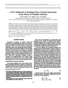
take longer than nonprocess (control) conditions, and assuming that perceived time and effort are directly related to real time and effort, we hypothesized that the phased conditions would lead not only to an increase in total decision time, but also to more total acquisitions, more attributes examined per alternative, more time spent per alternative examined, and a higher number of acquisitions made per attribute examined. Method Subjects Forty-nine students from 3rd and 4th year pharmacy classes at the University of Toronto were randomly assigned to the phased specified (n 5 16), the phased unspecified (n 5 17), and the control (final choice only; n 5 16) conditions. The subjects’ task was to put themselves in the place of a graduating pharmacy student who was interested in going to graduate school in pharmacy and then to decide which school or schools to apply to. The subjects were tested individually and received a cash payment of $10 for their participation. The entire experimental session took approximately 30 min. Stimuli Sixteen graduate school options were presented, and each option was described by its tuition costs ($3,500 or $6,000 per year), its geographical location with respect to Toronto (in Toronto or 1,000 km from Toronto), its reputation (top 10%, 20%, 30%, or 40% of graduate programs in the country), its selectivity in admitting applicants (admitting the top 5%, 15%, 25%, or 35% of its applicants), the likableness of the potential advisor (somewhat or very likable, as rated by former graduate students), the likableness of his/her ongoing research (somewhat or very interesting), the amount of stipend offered ($12,000 or $16,500 per year), and whether or not the GRE exam was required for admission (required or not required). Half the options were presented with complete information such that reputation and selectivity were perfectly correlated and no option dominated the other options. The remaining eight options were identical to the first eight, but were presented with missing information such that one attribute (either reputation or selectivity) was listed as “unavailable” ; the use of missing attribute values lent additional realism to the task. Process Methodology Information acquisition and search behavior were monitored with the software system MouseTrace (Jasper & Shapiro, 2001). MouseTrace is a Windows version of another system called MouseLab (Johnson, Payne, Schkade, & Bettman, 1991); MouseTrace is easier to use for both subjects and experimenters, it accommodates significantly more information than does MouseLab, and most important for our present purposes, it allowed for multiple responses as well as multiple decision stages. 7 MouseTrace uses computer graphics to display available stimuli in an alternative 3 attribute matrix (or grid) of information. When a set of options first appears on the screen, the values for each alternative– attribute combination are “hidden” behind the boxes (or cells) of the resulting matrix. To open a particular box and examine the information, the subject has to move the cursor via the mouse into the box. In Experiment 2, the subject had to click the mouse button to open a box and click again to close it; only one box could be opened at a time. The subjects were asked to choose an alternative (or alternatives, in the phased conditions) after selecting as many information boxes as they desired; options were chosen by clicking on the alternative name in the matrix itself. In terms of raw data, MouseTrace records the identity of the boxes that are opened and closed, the length of time that the boxes are opened (measured to one thousandth of a second), the order in which the boxes are opened, the length of time between the closing of one

VALIDATING A NEW PROCESS TRACING METHOD

505

box and the opening of another, the alternative(s) chosen at each stage and the times at which they are chosen, the order in which alternatives are selected and unselected, and the total decision time for each stage and the entire task.

number of acquisitions made per attribute examined, the average number of attributes examined per alternative, the relative importance of each attribute as assessed through attribute values, and the distribution of options chosen.

Dependent/Process Measures These data are used to derive a variety of process measures, including measures related to depth, sequence, and content. Depth measures refer to the amount of information accessed from the available information environment and are often associated with effort. Experiment 2 utilizes three such measures: the total number of information items accessed (acquisitions), the decision time, and the average time spent per item of information acquired. Sequence measures generally refer to the temporal pattern in which information is acquired and assessed through a comparison of the nth and the nth + 1 pieces of information searched. Here we use one primary measure —search pattern (or transition index) —a measure of the relative number of alternative-based (same alternative but different attribute) and attribute-based (same attribute but different alternative) transitions; the measure was originally developed by Payne (1976) and later modified by Bockenholt and Hynan (1994). A more positive number indicates relatively more alternative-based (compensatory) processing; a more negative number indicates relatively more attribute-based (noncompensator y) processing. A related measure, selectivity, assesses the variance in the proportion of time spent on each alternative; compensatory processing implies a pattern of information acquisition that is low in variance across alternatives, whereas noncompensatory strategies imply higher variance. Finally, content measures refer to exactly what information is acquired and which option(s) are chosen. Indices in Experiment 2 include the average time spent per alternative examined, the average

Procedure Except for the change from automobiles to graduate schools and from a paper and pencil to a computerized information monitoring task, the instructions for the choice task were virtually identical in Experiments 1 and 2. Following an initial cover story and an introduction to MouseTrace and its features (including a tutorial involving choices between automobiles), subjects were presented with a matrix similar to that shown in Figure 1. The subjects in the control condition were told to examine the 16 options carefully, to view as much or as little information as they desired, and to select the one school that they thought would be their first choice. The subjects in the phased conditions were asked in Stage 1 to select the universities that they would be interested in looking at if they were “window shopping” for a university—that is, the “ones that you would probably send away for catalogs describing their programs”— and in Stage 2 to select the universities that they would seriously consider applying to—that is, the “ones that you would want to visit personally.” In Stage 3, they were asked to indicate the one that they would actually select. Instructions were identical for these two conditions except for the number of options to choose—in one case, the subjects were required to narrow the original set of options to a specific a priori number in each of the three stages (6, 3, and 1), whereas in the other, the subjects were allowed to narrow as quickly or as slowly as they wanted across the three stages. Following the choice task, all subjects completed an attitudinal questionnaire similar to the one used in Experiment 1 and estimated (on a scale of 1 to 10) the importance that they placed on each attribute.

Figure 1. Sample MouseTrace matrix screen from Experiment 2.

506

JASPER AND LEVIN

Results The results will be presented in three sections. The first parallels the results section of Experiment 1 and examines the differences among the three conditions in terms of final choice, the attitudinal items, and the relationship between the derived attribute standard scores and subjects’ selfestimates of attribute importance. The second section compares the conditionsacross a variety of aggregate or overall process measures. The third focuses on stage-related effects and assesses temporal changes, using the same set of processing measures. Choices, Attitudes, and Self-Estimated Attribute Weights As in Experiment 1, the subjects’ choices in Experiment 2 were compared across conditions and stages, using attribute standard scores as the dependent variable. The scores for final choice are shown in Table 5. These scores were submitted to a 3 (condition)3 8 (attribute) ANOVA.8 The attribute main effect was significant [F(7,296) 5 8.18, p , .001], while the condition main effect and attribute 3 condition interaction were nonsignif icant [F(2,44) 5 1.69 and F(14,296) 5 1.05, respectively], indicating that the attributes were weighted differently and that all three conditions were comparable in terms of final choice based on attribute standard scores. Graduate school location, stipend amount, and reputation were consistently near the top in terms of attribute importance, while tuition cost and research likableness were consistently near the bottom. A comparison of attribute standard scores across stages for the two phased conditionsalso yielded results very similar to those for Experiment 1. The attribute main effect and attribute 3 decision stage interaction were significant [F(7,217) 5 8.72 and F(14,413) 5 7.10, respectively, p , .001 in both cases], while all other effects were nonsignificant. Thus, as in Experiment 1, it appears that in Experiment 2 the two phased conditions were equivalent in their ability to detect changes in attribute standard scores across

stages. The only notable difference between the two experiments was the nature of the attribute 3 decision stage interaction. In Experiment 1, the attribute that was most important in Stage 1 increased in importance over stages while the attribute that was least important in Stage 1 decreased in importance over stages. In Experiment 2, the two attributes that were most important in Stage 1 (reputation and stipend) remained unchanged in terms of importance while the other six attributes experienced fairly dramatic shifts across stages (tuition, location, selectivity, research likableness, and GRE increased in importance while advisor likeableness decreased). Important to note is that in both experiments, the interaction (regardless of its form) did not differ across conditions, as was indicated by a nonsignificant triple interaction of attribute 3 condition 3 decision stage [F(14,413) 5 1.20, in Experiment 2]. The subjects’ self-estimates of the importance of these attributes appear in Table 6. What stands out immediately is that the patterns of self-estimated weights and attribute standard scores (Table 5) do not match perfectly. In fact, the patterns are fairly dissimilar for all three conditions. As in Experiment 1, correlations were computed for each subject between the attribute standard scores in final choice and the self-estimated attribute weights. The mean correlation was .32 in the unphased condition, .30 in the phased unspecified condition, and .19 in the phased specified condition.These correlations are substantially lower than those in Experiment 1, primarily because there were more attributes to attend to. However, as in Experiment 1, an ANOVA indicated that the correlations were not significantly different from each other [F(2,44) 5 .83]. Finally, the attitudes and perceptions of subjects toward the three conditions in Experiment 2 were much like those in Experiment 1; thus, they will not be reported in detail here. Univariate ANOVAs revealed that there were no significant differences between the conditions.Two items, however, approached significance, suggesting that the phased paradigm (specified or unspecified) may lead to increased confidence and/or satisfaction in one’s deci-

Table 5 Mean Attribute Standard Scores For Final Choice in Experiment 2 Condition Phased Specified (n 5 16) Attribute Stipend (St) Tuition (T) Location (L) Reputation (Re)* Selectivity (Se)† Advisor (A) Research (Rs) GRE (G) Order of importance

M

Phased Unspecified (n 5 15) SE

.625 .806 -.625 .806 .625 .806 .056 .978 -.030 1.01 0 1.03 0 1.03 .375 .957 L St G Re A Rs Se T

M

SE

.467 .915 -.600 .828 .600 .828 .383 1.08 .335 1.11 .200 1.01 -.200 1.01 .067 1.03 L St Re Se A G Rs T

Unphased (n 5 16) M

SE

.625 .806 -.625 .806 .625 .806 .727 .630 -.791 .582 0 1.03 0 1.03 -.125 1.02 Re St L A Rs G T Se

*Sample size for the phased unspecified condition equals 14. †Sample size for the phased specified, phased unspecified, and unphased conditions equals 15, 8, and 13, respectively. Data points were lost because of “unavailable” or missing information.

VALIDATING A NEW PROCESS TRACING METHOD

507

Table 6 Self-Estimated Attribute Weights in Experiment 2 Condition Phased Specified (n 5 16) Attribute

M

Stipend (St) Tuition (T) Location (L) Reputation (Re) Selectivity (Se) Advisor (A) Research (Rs) GRE (G) Order of importance

Phased Unspecified (n 5 17) SE

M

7.00 2.58 5.88 2.55 5.31 3.00 7.44 2.19 7.00 1.97 8.19 1.52 7.25 2.02 4.38 3.20 A Re Rs Se St T L G

Unphased (n 5 16)

SE

5.94 2.10 5.70 1.83 5.65 3.37 7.94 2.33 6.12 2.29 8.12 1.87 8.06 1.34 4.12 2.76 A Rs Re Se St T L G

sion [F(2,46) 5 2.76 and F(2,46) 5 2.67, respectively, p , .10 in both cases]. Overall Process Measures The main focus of this section concerns how people adapt to the graduate school choice task under the context of each condition. Effects are examined for three types of dependent process measures: amount, selectivity, and pattern of processing. For purposes of comparison, data are aggregated across stages for the two phased conditions. To fully characterize the effects of each condition, separate univariate analyses were conducted for each measure. Means are presented in Table 7. Asking subjects to go through stages was predicted to lead to an increase in total decision time, more acquisitions, greater search breadth and depth (i.e., more attributes examined and more time spent per alternative), and a higher number of acquisitions made per attribute examined (i.e., deeper attribute probing). No effects, how-

M

SE

4.44 2.96 4.31 3.30 5.81 2.71 8.44 1.21 7.75 1.34 7.19 2.51 7.75 1.81 2.94 2.46 Re Se Rs A L St T G

ever, were expected for the average time spent on each item of information acquired, selectivity in processing (i.e., variance in the proportion of time spent on each alternative), or the sequence in which information was acquired (based on Bockenholt and Hynan’s transition index). Our hypotheses were generally confirmed, but only for one phased condition. As predicted, there was a significant difference between conditions in terms of amount of processing and effort required. Effects were found for total decision time [F(2,46) 5 7.77, p , .01], number of acquisitions [F(2,46) 5 6.42, p , .01], search breadth [F(2,46) 5 2.54, p , .10], search depth [F(2,46) 5 5.69 and F(2,46) 5 5.74, open box time per alternative and per attribute, respectively, p , .01 in both cases], and attribute probe [F(2,46) 5 4.57, p , .05]. However, follow-up analyses revealed that the phased specified condition was largely responsible for these effects. Statistically, the phased unspecified condition was no different than the unphased (control) condition on any of the aforementioned mea-

Table 7 Mean Information Processing Measures as a Function of Condition Condition Phased Specified (n 5 16) Process Measure Breadth (no. attributes/ alternative examined) Depth (open box time/ alternative examined) Depth (open box time/ attribute examined) Attribute probe (no. acquisitions/ attribute examined) Transition index Selectivity (variance in proportion of open box time/alternative) Total number of acquisitions Total decision time Total open box time Open box time/acquisition

Phased Unspecified (n 5 17)

Unphased Control (n 5 16)

M

SE

M

SE

M

SE

5.98

1.22

5.18

1.41

4.88

1.64

*

18.42

8.98

12.07

5.86

10.63

5.65

***

36.85

17.95

23.95

11.83

21.20

11.32

***

37.18 10.93

23.93 12.27

26.02 11.47

11.30 11.72

19.97 13.47

10.47 12.18

**

0.0024 319.88 701.32 294.80 0.97

0.0011 189.45 311.11 143.62 0.25

0.0037 208.12 457.14 191.63 0.94

0.0024 90.41 184.01 94.67 0.27

0.0042 159.75 390.24 169.59 1.10

0.0023 83.78 192.67 90.60 0.44

** *** *** ***

*Significantly different, p , .10. **Significantly different, p , .05.

***Significantly different, p , .01.

508

JASPER AND LEVIN

sures. Significantly less effort was used and less information was processed in these conditions as compared with the phased specified condition. The pattern of results for the remaining variables also was largely as predicted. There was no difference in terms of average time spent on each item of information acquired [F(2,46) 5 1.02] or the overall sequence in which the information was acquired [F(2,46) 5 .20]. Subjects spent approximately 1 sec per acquisition in all three conditions and utilized more alternative- than attribute-based processing throughout (as indicated by the relatively high positive transition index numbers). However, contrary to prediction, there was a significant difference in terms of selectivity in processing. Specifically, the variance in processing across alternatives differed across conditions [F(2,46) 5 3.61, p , .05]. As seen with previous measures, the effect was largely due to one condition—the

phased specified condition. Apparently, the effect of asking decision makers to narrow their choices, where subjects are asked to produce a specified number of alternatives at each stage, is to decrease one’s selectivity in processing. Stage-Related Process Comparisons As indicated previously, the strength of a phased approach lies in its ability to monitor temporal or stage-related changes in decision making. Thus, in this final section we concentrate on comparing the three conditions on their ability to detect changes in information processing across time. For the two phased conditions,the built-in stages will serve as our stopping points for measuring each process variable. For the unphased condition, it is a bit more complicated. Although there may be a number of solutions to creating a post hoc phased analogue of an unphased task, we have chosen to divide the data (i.e., the number of ac-

Table 8 Mean Information Processing Measures as a Function of Condition and Decision Stage Decision Stage Process Measure

Stage 1

Stage 2

Breadth (no. attributes/alternative examined) Phased specified (n 5 16) 5.80 6.31 Phased unspecified* 5.07 6.55 Unphased (n 5 16) 4.43 4.78 Depth (open box time/alternative examined) Phased specified (n 5 16) 13.16 9.55 Phased unspecified 8.53 7.57 Unphased (n 5 16) 7.73 5.61 Depth (open box time/attribute examined) Phased specified (n 5 16) 26.31 7.85 Phased unspecified 7.95 3.88 Unphased (n 5 15) 16.06 4.44 Attribute Probe (no. acquisitions/attribute examined) Phased specified (n 5 16) 23.04 10.62 Phased unspecified 17.64 6.54 Unphased (n 5 16) 13.18 4.88 Transition Index Phased specified (n 5 16) 10.82 1.04 Phased unspecified 10.99 0 Unphased (n 5 16) 7.78 6.77 Selectivity (variance in proportion of open box time/alternative) Phased specified (n 5 16) .0017 .0061 Phased unspecified .0025 .0076 Unphased (n 5 15) .0039 .0237 Total Number of Acquisitions Phased specified (n 5 16) 199.38 79.62 Phased unspecified 135.93 47.67 Unphased (n 5 16) 100.75 37.75 Total Decision Time Phased specified (n 5 16) 495.00 138.11 Phased unspecified 317.81 95.68 Unphased (n = 16) 264.44 73.39 Total Open Box Time Phased specified (n 5 16) 210.51 57.33 Phased unspecified 133.65 38.42 Unphased (n 5 16) 118.27 33.21 Open Box Time/Acquisition Phased specified (n = 16) 1.11 .77 Phased unspecified 1.03 .77 Unphased (n 5 16) 1.22 .90

Stage 3 7.06 6.17 5.51 8.99 7.19 6.21 3.38 3.18 2.50 5.06 3.89 2.77 -1.82 .85 3.12 .0148 .0260 .0565 40.88 29.60 21.25 68.20 60.01 52.43 26.96 22.28 18.42 .66 .94 .88

*Sample size for the phased unspecified condition equals 17, 16, and 15 for Stages 1, 2, and 3, respectively, for all process measures.

VALIDATING A NEW PROCESS TRACING METHOD quisitions) on the basis of the proportionate number of acquisitions made in the two phased conditions combined. For example, Subject 2 in the control condition made 168 total acquisitions. The average numbers of acquisitions made in Stages 1, 2, and 3 for all participants in the phased conditions were 168.2, 62.8, and 35.4, respectively; the correspondent proportions are 63.1%, 23.6%, and 13.3%. Thus, for Subject 2, we divided the 168 total acquisitions into three groups—the first 106 acquisitions, the middle 40 acquisitions, and the last 22 acquisitions. We also assumed that Subject 1 narrowed his/her alternativesfrom 16 to 4 in Stage 1, 4 to 3 in Stage 2, and 3 to 1 in Stage 3. We based the latter assumption on the number of rows (alternatives) Subject 2 examined at each stage. This assumption is particularly crucial when one is calculating the Bockenholt and Hynan transition index.9 The means for each process measure are shown in Table 8. A significant condition 3 decision stage interaction [F(4,88) 5 2.99, p , .05] was found when transition indices were submitted to a 3 (condition)3 3 (decision stage) ANOVA. While all three conditions revealed a shift from a positive (or less negative) to a negative (or less positive) index, suggesting a shift from more compensatory to more noncompensatory(less compensatory) decision strategies, the control condition showed a less pronounced effect than did the phased conditions. In fact, when we conducted the same analysis with an equal (rather than proportionate) number of acquisitions at each stage, subjects in the control conditiondemonstratedthe reverse pattern—a shift from a negative (or less positive) to a positive (or less negative) transition index, which replicates the work of Payne and his colleagues (Payne, Bettman, & Johnson, 1993). The selectivity measures are supportiveof the same finding; the interactionbetween conditionand decision stage was significant [F(4,86) 5 4.82, p , .01]. Although the variance in open box time per alternativeincreased across stages in all conditions, it increased at a faster rate for the control condition. Again, larger selectivity numbers are indicative of more noncompensatory(less compensatory) processing. The remaining process measures help to distinguish between the three conditions as well. As with the measures above, a univariate ANOVA was conducted with condition (3 levels) and decision stage (3 levels) as factors. Two effects, in particular, will be emphasized here: the decision stage main effect and the condition 3 decision stage interaction. Effort. Subjects in all conditions spent approximately five to eight times as much time (total decision time and open box time) and made about four to five times as many acquisitions of separate pieces of information in Stage 1 than in Stage 3 [F(2,88) 5 158.47, F(2,88) 5 136.77, and F(2,88) 5 108.00, respectively; p , .001, in each case]. However, there was a tendency for these measures to decrease more rapidly across stages in the phased specified condition than in the other two conditions,as can be seen in significant condition 3 decision stage interactions [F(4,88) 5 7.21, p , .001, F(4,88) 5 5.32, p , .001, and F(4,88) 5 4.30, respectively, p , .01]. Subjects also spent

509

10%– 40% less open box time per acquisition in Stage 3 than in Stage 1 [F(2,88) 5 11.32, p , .001]; in this case, though,there was no interaction between condition and decision stage [F(4,88) 5 1.11]. Depth of search. Subjects in the three conditions spent 20%–50% more time examining each alternative in Stage 1 than in Stage 3 [F(2,88) 5 5.84, p , .01]. Nevertheless, there was no significant condition 3 decision stage interaction [F(4,88) 5 .85]. Subjects also demonstrated a similar pattern in terms of time spent on each attribute. Approximately three to eight times as much time was spent by subjects examining each attribute in Stage 1 than in Stage 3 [F(2,86) 5 141.79, p , .001]. For this measure, however, the interaction was significant [F(4,86) 5 4.04, p , .01], showing that the difference in depth of search between the phased specified and the other two conditions was especially evident early in the decision process. Breadth of search. Subjects in the three conditions examined significantly more attributes per alternative in Stage 3 than in Stage 1 [F(2,88) 5 9.35, p , .001], suggesting that decision makers search with more breadth the closer one gets to a final decision. Although phased specified subjects tended to examine more attributes per alternative than did the other subjects, as can be seen in the main effect of condition [F(2,44) 5 2.46, p , .01], there was no interaction between condition and decision stage [F(4,88) 5 1.19]. Attribute probe. Subjects acquired significantly more information about each attribute examined in Stage 1 than in Stage 3 [F(2,88) 5 104.28, p , .001]. There was also a marginally significant interaction between condition and decision stage [F(4,88) 5 2.46, p , .10], suggesting differential rates of probing across stages with the difference in attribute probing being particularly pronounced in Stages 1 and 2. Discussion The results of Experiment 2 replicated the main results of Experiment 1 within a new stimulus domain, with a different number of options and attributes, and within the context of a computerized (rather than a paper and pencil) task designed to monitor traditional process variables. Like Experiment 1, Experiment 2 revealed that asking individualsto go through stages does not necessarily alter their final choices. In Experiment 1, this was true for the phased unspecified condition (in comparison with the unphased condition); in Experiment 2, this was true for both the phased specified and phased unspecified conditions. In addition,there were no detectable differences among the three conditions in terms of subjects’ perceptions of the task or the convergence of derived attribute standard scores and subjects’ self-estimated attribute weights. The only notable differences between the two experiments were the relatively low correlations between the standard scores and self-estimates and the marginally significant effects in confidence and satisfaction ratings, both seen in Experiment 2. The results of Experiment 2 also extended those of Experiment 1. By measuring traditional process variables, we

510

JASPER AND LEVIN

found that in terms of aggregate measures, the phased unspecified and unphased (control) conditions were indistinguishable. Specifically, no differences were detected between these two conditions in terms of total number of acquisitions,total decision time, total open box time, open box time per acquisition, breadth or depth of search, attribute probe, selectivity, or the transition index that served as an indicator of search pattern. The same could not be said of the phased specified condition, which differed in every respect except the aggregate transition index and open box time per acquisition. Because of the more stringent requirements, subjects in the phased specified condition appeared to work harder than subjects in either of the other conditions. The phased specified condition also differed from the other two conditions with respect to many of the temporal or stage-related process measures. Although all three conditions showed a decrease across stages in number of acquisitions, decision time, open box time, and depth of search (i.e., time spent on each attribute), the phased specified condition showed a much more rapid decrease in all of these measures; Stage 1 was responsible for much of this difference. Interestingly enough, the only measures that revealed a process difference between the phased unspecified and unphased conditions were the temporal transition and selectivity measures. In both cases, the phased unspecified and unphased conditions (along with the phased specified condition) showed a shift from more to less compensatory (alternative-based) processing, but it was less pronounced in the control condition. This shift is at odds with previous research (using unphased conditions), which has shown evidence of a shift from more noncompensatory to more compensatory processing. We suspect that it has something to do with task structure (i.e., the alternative 3 attribute axes) and the natural human tendency (at least for those proficient in English) to read left to right. In the present task, attributes were on the x-axis (across the top) and alternativeswere on the y-axis (down the left side). When confronted with a new matrix of information, and if one is unsure where to begin (e.g., one is undecided as to the most important attribute), a common strategy may be to start with the first row (alternative) and begin opening boxes left to right. This, by definition, is a compensatory strategy; however, subjects may not be making, intentionally, tradeoffs between attributes. Nevertheless, this will increase the transition index values. After familiarizing themselves with the matrix, subjects may then begin attending to key attributes across alternatives,which will serve to lower the index values. If this is true, one would predict that if the axes were reversed, the opposite effect would be shown—a shift from more noncompensatory to compensatory processing.10 GENERAL DISCUSSIO N In closing, what we have tried to do here is to describe and validate a technique (or paradigm) which is objective and easy to use and which provides researchers with valu-

able process information. We believe that this may well represent the most complete set of validity tests in the process tracing literature, and we encourage those using other methods to follow suit. The question that we have attempted to answer is the following: Does phased narrowing distort the processes it is designed to uncover? Two experiments were conducted, comparing the following three conditions: a group in which subjects were required to narrow their multiattribute options by using specified numbers at each of three stages; a group in which subjects were required to narrow the same alternatives according to the same instructions, but by using unspecified numbers; and a control group of subjects who were asked simply to make a final choice, without mention of stages. In Experiment 1, no difference was found between conditions with respect to the attitudes and perceptions of the decision maker (save for the perceived time to complete the task), the convergence between attribute standard scores (Levin and Jasper’s measure of attribute importance) and subjects’ self-estimated attribute weights, and the ability to detect an established relationship between attribute standard scores and an individual difference measure—namely, nationalism. However, there were slight differences between conditions in terms of final choice. Specifically, the phased specified condition was found to differ from the phased unspecified and unphased conditions, which were not different from each other. Experiment 2 tended to corroborate this pattern of results. Again, no difference was found between conditions in terms of the attitudes and perceptions of the decision maker and the convergence between attribute standard scores and subjects’ self-estimated attribute weights. In addition, unlike in Experiment 1, no differences were uncovered in Experiment 2 with respect to the distributionof final choices. Nevertheless, many differences were found between the conditions in terms of traditional process variables, and the vast majority of these findings singled out the phased specified condition as being different from the other two conditions. More specifically, subjects in the phased specified condition spent more time looking at information and making their final decision, made a greater number of acquisitions (i.e., looked at more information), searched that information with greater breadth and depth, and probed more deeply into each of the attributes. In addition, although all three conditions demonstrated a decrease in decision time, open box time, and time spent per attribute examined (depth of search) across time, these measures decreased more rapidly across stages in the phased specified condition than in the other two conditions. Taken together, the present results provide strong evidence that if one wants to use phased narrowing to study decision making, then allowing decision makers to determine their own set sizes enroute to making a final decision is the method of choice. The method does not appear to distort the processes that it is designed to uncover, and at the same time, it can allow one to (1) analyze how the impact of each attribute changes as the decision maker

VALIDATING A NEW PROCESS TRACING METHOD approaches a final choice, (2) compare attribute importance within a stage as well as across stages, and (3) examine each of the above at the level of the individual decision maker. Furthermore, the unspecified version allows set size to be used as a dependent variable. We have found this to be particularly useful, for example, in the comparison of inclusion and exclusion decision processes: We have found that subjects instructed to indicate which options they would include for further consideration narrowed their choices more than did subjects instructed to indicate which options they would exclude from further consideration (Levin, Huneke, & Jasper, 2000; Levin, Jasper, & Forbes, 1998), and phased narrowing was instrumental in explaining why. We are not suggesting, however, that phased narrowing can be used in every situation. It may well be that under some contexts, the phased unspecified condition may distort decision processes, and that under other contexts, it may produce a different decision than would another method (e.g., a method that would permit any of the original options to emerge at any point). We are also not suggesting that requiring subjects to narrow their options by using a priori specified numbers at each stage (i.e., the phased specified condition) is a completely useless procedure. There may be situationsin which that particular set of instructions is the natural context, such as when budgetary constraints necessitate that one narrow down to a fixed number of interviews for a job. Furthermore, the finding that such a condition may change one’s processes and/or final decision does not preclude that condition from being used as a decision aid. Decision aids, by their very nature, are designed to change (and improve) decisions. Thus, with future research, decision researchers may find that the phased specified condition is a valuable tool for that endeavor. We will argue, though, that either version of phased narrowing seems particularly well suited for decisions that require a fair amount of forethought and naturally involve discrete steps in which the formation of earlier choice sets precedes the final choice. We have shown that the phased narrowing method is apt to alter the decision process, but only when the subject is restricted by number of options and the number specified may deviate considerably from the number that would have been chosen had the subject not been constrained. Future research should clarify other conditions under which distortions and/or decision changes are likely to occur. In the meantime, researchers who plan to use the method to study decision processes under similar environments should feel confident in using the technique. When combined with an information monitoring program such as MouseTrace, it offers a rich array of prechoice data for understanding decision behavior. REFERENCES Anderson, N. H. (1982). Methods of information integration theory. New York: Academic Press. Anderson, N. H., & Zalinski, J. (1988). Functional measurement ap-

511

proach to self-estimation in multiattribute evaluation. Journal of Behavioral Decision Making, 1, 191-221. Beach, L. R. (1993). Broadening the definition of decision making: The role of prechoice screening of options. Psychological Science, 4, 215-220. Bockenholt, U., & Hynan, L. S. (1994). Caveats on a process tracing measure and a remedy. Journal of Behavioral Decision Making, 1, 103-117. Carroll, J. S., & Payne, J. M. (1977). Judgements about crime and the criminal: A model and a method for investigating parole decisions. In B. D. Sales (Ed.), Perspectives in law and psychology: The criminal justice system (Vol. 1, pp. 41-55). New York: Plenum. Ericsson, K. A., & Simon, H. A. (1993). Protocol analysis: Verbal reports as data (rev. ed.). Cambridge, MA: MIT Press. Fidler, E. J. (1983). The reliability and validity of concurrent, retrospective, and interpretive verbal reports: An experimental study. In P. Humphreys, O. Svenson, & A. Vari (Eds.), Analysing and aiding decision processes (pp. 429-440). Amsterdam: Elsevier. Jasper, J. D. (2002). How people deal with missing information: Insights from process tracing. Manuscript in preparation. Jasper, J. D., & Shapiro, J. (2001). MouseTrace: A better mousetrap for catching decision processes. Manuscript submitted for publication. Johnson, E. J., Payne, J. W., Schkade, D. A., & Bettman, J. R. (1991). Monitoringinformation processing and decisions: The Mouselab system. Unpublished manuscript. Durham, NC: Duke University, Fuqua School of Business, Center for Decision Studies. Judd, C. M., & McClelland, G. H. (1989). Data analysis: A modelcomparison approach. San Diego, CA: Harcourt Brace Jovanovich. Levin, I. P., Huneke, M. E., & Jasper, J. D. (2000). Information processing at successive stages of decision making: Need-for-cognition and inclusion-exclusion effects. Organizational Behavior & Human Decision Processes, 82, 171-193. Levin, I. P., & Jasper, J. D. (1995). Phased narrowing: A new process tracing method for decision making. Organizational Behavior & Human Decision Processes, 64, 1-8. Levin, I. P., & Jasper, J. D. (1996). An experimental analysis of nationalistic tendencies in consumer decision processes: The case of the multi-national product. Journal of Experimental Psychology: Applied, 2, 17-30. Levin, I. P., Jasper, J. D., & Forbes, W. S. (1998). Choosing versus rejecting options at different stages of decision making. Journal of Behavioral Decision Making, 11, 193-210. Levin, I. P., Jasper, J. D., & Gaeth, G. J. (1996). Measuring the effects of framing country-of-origin information: A process tracing approach. Advances in Consumer Research, 23, 385-389. Levin, I. P., Jasper, J. D., Mittelstaedt, J. D., & Gaeth, G. J. (1993). Attitudes toward “buy America first” and preferences for American and Japanese cars: A different role for country-of-origininformation. Advances in Consumer Research, 20, 625-629. Levin, I. P., Johnson, R. D., & Jasper, J. D. (December, 1993). The role of nationalism in the consumer choice process: Comparison between the U. S. and Canada. In G. S. Albaum et al. (Eds.), Proceedings of the Fourth Symposium on Cross-Cultural Consumer and Business Studies. Nedungadi, P. (1990). Recall and consumer consideration sets: Influencing choices without altering brand evaluations. Journal of Consumer Research, 17, 245-253. Olshavsky, R. W. (1979). Task complexity and contingent processing in decision making: A replication and extension. Organizational Behavior & Human Performance, 24, 300-316. Payne, J. W. (1976). Task complexity and contingent processing in decision making: An information search and protocol analysis. Organizational Behavior & Human Performance, 16, 366-387. Payne, J. W., Bettman, J. R., & Johnson, E. J. (1988). Adaptive strategy selection in decision making. Journal of Experimental Psychology: Learning, Memory, & Cognition, 14, 534-552. Payne, J. W., Bettman, J. R., & Johnson, E. J. (1993). The adaptive decision maker. Cambridge: Cambridge University Press. Roberts, J. [H.] (1989). A grounded model of consideration set size and composition. Advances in Consumer Research, 16, 749-757.

512

JASPER AND LEVIN

Roberts, J. H., & Lattin, J. M. (1991). Development and testing of a model of consideration set composition. Journal of Marketing Research, 28, 429-440. Shimp, T. A., & Sharma, S. (1987). Consumer ethnocentrism: Construction and validation of the CETSCALE. Journal of Marketing Research, 24, 280-289. Shocker,A. D., Ben-Akiva, M., Boccara,B., & Nedungadi,P. (1991). Consideration set influences on consumer decision-making and choice: Issues, models, and suggestions. Marketing Letters, 2, 181-197. Slovic, P., & Lichtenstein, S. (1971). Comparison of Bayesian and regression approaches to the study of information processing in judgment. Organizational Behavior & Human Performance, 6, 649-744. Smead, R. J., Wilcox, J. B., & Wilkes, R. E. (1981). How valid are product descriptions and protocols in choice experiments? Journal of Consumer Research, 8, 37-42. Zhu, S., & Anderson, N. H. (1991). Self-estimation of weight parameter in multi-attribute analysis. Organizational Behavior & Human Decision Processes, 48, 36-54. NOTES 1. The attributes, their description, and their corresponding values (except for % American workers) were adapted from the Annual Car Guide put out by Consumer Reports. 2. Ratings (on scales of 1 to 10) were used instead of asking subjects to allocate (e.g., 100) points, because Zhu and Anderson (1991) have found the allocation procedure to be less valid than the rating procedure. Following Zhu and Anderson, these ratings were completed after the choice task, to provide subjects with a context for making these ratings which included attribute levels and combinations. 3. Three attributes instead of four were used in this and all subsequent analyses, because attribute standard scores are not independent (i.e., they sum to zero). The fourth is a linear combination of the other three. The three attributes used were reliability, price, and % American workers. 4. Two subjects were dropped from these analyses, because of missing data. Although, for statistical purposes, we used attribute standard scores rather than discrete choices to compare conditions on both final choice and the choice set of three, we thought that it might be of some value to look at the frequency data as well. No formal analyses were conducted; descriptively, however, these data match up nicely with the results just mentioned. Specifically, in terms of final choice, Brand B was the most popular option across all three conditions, followed by Brand A and then Brand H in the phased specified and phased unspecified conditions and Brand H and then Brand A in the unphased condition. For the choice set of three, the top four choices (in order from top to bottom) were ABGH, BAHG, and BAHG, for the phased specified, phased unspecified, and unphased conditions, respectively. (A complete table of the choice distributions for each condition is available to interested readers. Please contact the first author.) The “contrived” second stage allows us to make stage-like comparisons across all three conditions. This is especially important for the control condition, which has no “built-in” stages. A valid concern that one might have about this “contrived” second stage is whether or not the first, second, and third choices corresponded to those made in Stage 2 of the phased conditions. To allay these fears, the answer is a resounding “yes.” In only 1 case out of 48 did the choices not match up.

5. Although the attribute 3 condition 3 decision stage interaction was nonsignificant, the F value did approach significance ( p , .10). Follow-up analyses comparing the two phased conditions at each stage separately indicated that the attribute 3 condition interaction was significant only in Stages 2 and 3 [F(2,92) 5 6.62 and F(2,92) 5 5.65, respectively, p , .01 in both cases]. Although it is not discussed, we also compared the set sizes of the two phased conditions across stages. The mean numbers of options chosen in the phased specified condition were 6.0, 3.0, and 1.0, for Stages 1, 2, and 3, respectively. For the phased unspecified condition, the means were 6.1, 3.1, and 1.0. 6. Experiment 2 was actually part of a larger study investigating not only the validity of phased narrowing, but also the effects of inclusion/ exclusion and missing information on decisions and decision processes. Specifically, half of the subjects were asked (as in Experiment 1) to include the options that they would consider in later stages, while the other half were asked to exclude the options that they would reject for consideration; all data reported in Experiment 2 are from the inclusion condition. In addition, half of the options in the initial choice set contained missing (or “unavailable”) information, while the other half contained complete information. In an effort to stay focused, we have chosen not to discuss the inclusion/exclusion or missing information results. The reader who is interested in these topics may be referred to other papers (e.g., Jasper, 2002). 7. One might correctly argue that it makes no sense to test the validity of a new method (phased narrowing) by using another method (MouseTrace) that has yet to be validated. However, we argue that MouseTrace is virtually identical to MouseLab in terms of its basic operation, and MouseLab has been validated and is widely accepted as the standard in information monitoring technology (see, e.g., Payne et al., 1988, p. 543). 8. In contrast to Experiment 1, attribute standard scores did not automatically sum to zero; therefore, all eight attributes were included in this and all subsequent analyses. For analytic purposes in calculating attribute standard scores, the sign was reversed for tuition, location, and reputation in such a way that positive values represented the selection of lower cost, closer, and more reputable graduate schools, respectively. 9. Other procedures include using the average number of options chosen in the two phased conditions (i.e., 6 to 3 to 1) and a constant number of options(i.e., 16). The latter is a reasonable option but may overestimate the true transition index. The former is also reasonable, but it becomes problematic (for some of the other process measures) when subjects examine more alternatives than average. It should be noted that neither of the procedures above changes the direction of the effects. It is also interesting to note that the mean numbers of rows examined in Stages 1 and 2 (6.81 and 3.31, respectively) of the control condition are very similar to the mean numbers of options selected in Stages 1 and 2 of the phased conditions; this increases our confidence in using this procedure. 10. We caution the reader that we are not making this argument in order to explain previous findings. Rather, we make it to possibly explain the present results. One might argue that practice would eliminate the effect. However, subjects were given a thoroughtutorial prior to the task. It is notable, though, that the training was with cars, not graduate schools. (Manuscript received July 7, 2000; accepted for publication December 22, 2000.)