Validating Model Clouds and Their Optical Properties Using

2006

MONTHLY WEATHER REVIEW

VOLUME 132

Validating Model Clouds and Their Optical Properties Using Geostationary Satellite Imagery ZHIAN SUN

AND

LAWRIE RIKUS

Bureau of Meteorology Research Centre, Melbourne, Victoria, Australia (Manuscript received 20 June 2003, in final form 29 November 2003) ABSTRACT A real-time validation scheme for diagnosing radiatively active clouds has been in operation for a number of years at the Australian Bureau of Meteorology. It compares IR channel imagery from four geostationary satellites and equivalent forward calculations using fields from the bureau’s global and regional NWP models. The scheme also attempts to glean some information about cloud amounts from the satellite data for direct comparison with the model but is hampered by the reliance on a single spectral channel. A new radiance code derived from the Edwards and Slingo radiation scheme and several cloud optical property schemes has recently been implemented into the system. The forward calculations were performed using both the operational radiative transfer code and this new code, and the results were compared with satellite measurements. The effects of different cloud optical property schemes, cloud particle scattering, and cloud phase state were investigated. The results have shown a dramatic improvement in the comparison due to changes in the model physical parameterizations. The major achievement obtained in this study is the implementation of a new ice water content diagnostic scheme developed on the basis of lidar–radar data collected at the Southern Great Plains, the cloud and radiation test bed site of the Atmospheric Radiation Measurement (ARM) Program in Oklahoma. Using this scheme in the cold cloud temperature region (T , 2508C) in conjunction with the new forward radiance code, the modeled brightness temperature using fields from the global NWP model is significantly improved.

1. Introduction A cloud-validating scheme was developed and has been running operationally at the Australian Bureau of Meteorology since the early 1990s (Rikus 1997). This scheme uses physical parameterizations identical to those used in the Bureau of Meteorology Global Assimilation and Prediction System (GASP) (Bourke et al. 1995) and the forecast fields from GASP to generate narrowband brightness temperatures (BTs) corresponding to a number of spectral infrared channels of geostationary satellites [e.g., Geostationary Meteorological Satellite (GMS), Geostationary Operational Environmental Satellite (GOES), and Meteosat]. The model cloud and radiation schemes are then validated by comparison of the modeled BT with the real satellite imagery. The geostationary satellites provide data for a large fraction of the globe at synoptic times corresponding to operational archive times; using geostationary satellites it is almost possible to obtain a synchronous global ‘‘image’’ (Rossow and Schiffer 1991). This is clearly desirable for the validation of a global model. The disadvantage of geostationary satellites is their limCorresponding author address: Z. Sun, BMRC, GPO Box 1289K, Melbourne VIC 3001, Australia. E-mail: [email protected]

q 2004 American Meteorological Society

ited number of spectral bands, which restricts the choice of model variables to be validated. Ideally, the choice would be for direct validation of cloud, but the limited spectral information available from the satellite precludes the use of accurate cloud identification schemes. Therefore it is better to use the model fields to generate radiance as seen by the satellite. Provided the offline code for the satellite infrared band and the model radiation code have comparable accuracy, disagreement between satellite and model-derived brightness temperature can then realistically be attributed to errors in the model’s thermodynamic and cloud fields. Over 10 yr of operation of the cloud validation scheme, a substantial amount of model data have been produced. Analysis of these results has shown that although the comparison of the model’s cloud fields with climatology may be considered adequate, real-time cloud fields are more difficult to characterize and validate, particularly if cloud optical properties are involved. Nevertheless it has been shown that the scheme is capable of providing useful and timely information about the operational medium-range prediction model and has also been used as a validation tool for the development of a modified diagnostic cloud scheme and various cloud optical property schemes implemented into the GASP model, leading to overall improvements in the model’s forecast performance.

AUGUST 2004

SUN AND RIKUS

One particular problem in the GASP system identified with this scheme is that the GASP model does not produce enough cold brightness temperatures in the Tropics (Rikus and Salby 2000); the satellite image shows an appreciable percentage of BTs below 200 K while the minimum model BTs are only around 220 K. It is suspected that this problem may be related to the cloud optical properties that are based on a temperature dependent cloud water/ice content parameterization (Lemus et al. 1997) and that may be inappropriate for thick high cloud. The offline code used to calculate the narrowband brightness temperature is derived from the two IR window bands of the Fels–Schwarzkopf radiation code (Schwarzkopf and Fels 1991, hereafter referred to as FS), which span the spectral region 800–990 cm 21 and include absorption due to the water vapor and its continuum determined by the Roberts scheme (Roberts et al. 1976). A new scheme based on the Edwards and Slingo (1996) radiation code has recently been implemented in the validation system in conjunction with several new cloud radiative parameterizations. The aim of this study is to test the new scheme with particular focus on the investigation of why the GASP system does not produce enough cold BTs. This is done by examining the effects due to cloud amount, height, cloud liquid/ice content, and different cloud optical property schemes. The paper is arranged as follows: the model and new cloud optical property schemes are introduced in section 2, and some offline comparisons are presented in section 3. The comparison between modeled and observed BT is given in section 4. Section 5 presents some forecast results using the GASP model supplemented with the new schemes examined in this study. Discussion and conclusions are presented in section 6. 2. Models The basic validation scheme has been detailed by Rikus (1997). Only a brief introduction to the new radiation code and cloud optical property schemes is given here. The new radiance code is derived from the Edwards and Slingo scheme (1996, hereafter referred to as ES). The code structure is essentially the same as the original code except for the changes required to calculate radiance rather than irradiance. In addition the treatment of the gaseous absorption and evaluation of the Planck function have also been modified. The gaseous absorption is now treated in terms of a correlated-k distribution method. For each satellite channel the spectral range is split into two bands and each band is further divided into 16 intervals chosen to have the modified half Gauss–Legendre quadrature spacing as suggested by Mlawer et al. (1997). The General Line-by-Line Atmospheric Transmittance and Radiance (GENLN2) model (Edwards 1992) is used to generate the gas ab-

2007

sorption coefficients k from the high-resolution transmission molecular absorption database (HITRAN96) (Rothman et al. 1998). A lookup table for k values at all quadrature points is set up for a number of reference pressures and temperatures as described by Mlawer et al. (1997). The k values corresponding to the actual pressure and temperature are obtained by linear interpolation from this table. The code currently includes three GMS-5 infrared satellite channels (channel 1 ranging over 805–900 cm 21 , channel 2 over 790–820 cm 21, and the water vapor channel over 1400–1500 cm 21 ), and more channels will be implemented later. The Clough water vapor continuum scheme (version 2.4) (Clough et al. 1989) is used in the calculations of the water vapor continuum absorption. The foreign broadening component of the continuum absorption is convolved with the calculations of the water vapor line absorption coefficient, and the self-broadening component of continuum absorption is treated separately, as described in Sun and Rikus (1999a). The calculations of the Planck function follow Mlawer et al. (1997). The satellite response function is applied to each spectral band as a weighting function. The BTs for the standard midlatitude summer and tropical atmospheres determined using this code were compared with those from the GENLN2 line-by-line code. The discrepancies for the three IR channels are all less than 0.1 K. Six cloud optical property schemes were implemented in the radiation code and are examined in this study, two schemes for liquid water clouds and four for ice clouds. The two liquid water cloud optical property schemes are those due to Sun and Shine (1994, hereafter referred to as SS) and Hu and Stamnes (1993, hereafter referred to as HS). The SS scheme parameterizes the single-scattering properties of water cloud in terms of cloud liquid water content (LWC) only for the 11-mm window region. Therefore it can be directly applied to the two infrared window channels, but some modifications may be needed for the water vapor channel. The HS scheme parameterizes the single-scattering properties in terms of cloud LWC and effective radius. The coefficients for the parameterizations were provided by Stamnes (1993) at high spectral resolution and have to be averaged across the spectral bands to derive the values required by a broadband code. We have found that using the coefficients derived by directly averaging these coefficients across spectral bands cannot reproduce the single-scattering parameters presented by Hu and Stamnes (1993) because of the nonlinear variation of these coefficients with wavelength. To solve this problem, we calculate the single-scattering parameters at high spectral resolution and average the results across the spectral band, weighted by the Planck function at 250 K. The coefficients corresponding to each spectral band are then determined by fitting these averaged parameters in terms of the equations given by Hu and Stamnes. Using this method we successfully reproduce

2008

MONTHLY WEATHER REVIEW

the single-scattering parameters presented by Hu and Stamnes. The four ice cloud optical property schemes are those due to Sun and Shine (1994, 1995), Fu et al. (1998), Kristjansson et al. (1999, hereafter KEM), and Ebert and Curry (1992, hereafter EC). The first parameterization, developed by Sun and Shine (1994, 1995), parameterizes the single-scattering properties of cloud particles in terms of the ice water content only for the 11mm window region. Again it can be directly applied to GMS-5 window channels. It is also simple in that the ice particle size information is not required. The second scheme, developed by Fu et al., parameterizes the single-scattering properties at high spectral resolution using both the ice water content (IWC) and generalized effective size G e defined for hexagonal ice crystals. The technique for implementing this scheme in the broadband code is therefore the same as that for the HS scheme. The variable G e required by this scheme is not generally available in NWP/climate models. In order to solve this problem and implement the Fu et al. scheme in the Bureau’s NWP and climate models, Sun and Rikus (1999b) have developed a parameterization for G e in terms of cloud temperature and IWC that can be directly used in this study. The Kristjansson et al. scheme parameterizes the single-scattering properties in terms of the mean maximum dimension D of ice crystals defined by Mitchell et al. (1996); D is further parameterized in terms of cloud temperature, enabling it to be used directly in the model. The last scheme, described by Ebert and Curry, specifies the ice cloud absorption coefficient as a function of effective radius req defined in terms of the equivalent sphere having the same surface area as a hexagonal particle. There is a barrier to the use of this scheme in climate models because a corresponding parameterization for req is not available. When it is implemented in a climate model a constant req is normally assumed: for example, req 5 40 mm was used in the European Centre for Medium-Range Weather Forecasts (ECMWF) model (Morcrette 2002). Since the cloud absorption coefficient varies significantly with req as shown in Fig. 2 of Ebert and Curry (1992), the use of a constant req would certainly introduce a large uncertainty in the calculations. Morcrette (2002) has tested the Sun and Rikus parameterization for G e by applying it to the EC optical property scheme in the ECMWF model and found that the modeled longwave radiation at the highlatitude surfaces, particularly in the South Pole, is significantly improved compared with that using the fixed req . Although this is encouraging, our investigations have shown that G e cannot be simply set equal to req or converted to req with a conversion factor as suggested by Fu et al. (1998) because of the differences in the definitions and the particle size distributions used in deriving them. In the Fu et al. (1998) study, it was shown that G e can be expressed by

VOLUME 132

2Ï3 IWC , 3r i A c

Ge 5

(1)

where IWC is assumed to be determined by the total volume of hexagons, r i is the ice density, and A c is the total cross-sectional area of cloud particles. A similar expression, but for the effective radius r e , defined for equivalent ice spheres was given by Francis et al. (1994): re 5

3 IWC , 4ri A c

(2)

where IWC is assumed to be determined by the total volume of spheres. Comparing Eqs. (1) and (2) we obtain re 5

2Ï3 3

Ge .

(3)

This equation provides a convenient way to transfer these two variables. If req defined in the EC scheme was evaluated by integration over the radius of the equivalent spheres then it would agree with Eq. (2) and the application of Eq. (3) would be valid. However, req was determined by the integration over the particle length and the application of Eq. (3) in such a case is invalid. We have calculated the req and G e using the eight particle size distributions given by Heymsfield and Platt (1984) plus an additional two distributions from Heymsfield (1975) that were used by Ebert and Curry (1992) to generate their parameterization. The results show that the difference between these two variables is large and not a constant as indicated by Eq. (3). Consequently, we decided to parameterize req in terms of the IWC using the same particle size distributions as used by Ebert and Curry. The following expression is found to well represent the relationship between req and IWC determined by these size distributions: req 5

IWC , a 1 bIWC

(4)

where IWC (g m 23 ), a 5 1.0374 3 10 24 , b 5 7.3404 3 10 23 , and req (mm). Note that this equation has an advantage in that req has an upper limit of 137 mm, which is roughly the same as the valid upper limit from the size distributions used to develop the cloud optical property scheme. In GASP the cloud water content is determined by a temperature-dependent diagnostic scheme developed on the basis of several aircraft observations (e.g., Heymsfield and Platt 1984; Stephens and Platt 1987; Francis et al. 1994; McFarquhar and Heymsfield 1997). This scheme will be discussed in more detail in the next section. The effective radius of water cloud droplets is estimated using the Martin et al. (1994) scheme that was developed at the Met Office based on aircraft observations. This scheme, which depends on LWC and total droplet concentration, has been tested by Rotstayn

AUGUST 2004

SUN AND RIKUS

2009

(1997) in the Commonwealth Scientific and Industrial Research Organisation (CSIRO) GCM for climate simulations. He recommended the use of total droplet concentrations of 100 cm 23 over the ocean and 800 cm 23 over the land. The value used for the oceanic area has also been examined by comparing the radiative properties of stratocumulus clouds modeled using the Martin et al. scheme with observations from aircraft (Sun and Pethick 2002). A good agreement was found. These two values have therefore been adopted in the Bureau’s NWP and climate models and are also used in the current application. Finally the liquid fraction in mixed-phase clouds is determined from the cloud temperature using a formula derived by Moss and Johnson (1994). 3. Some offline results Some offline calculations were performed for the purpose of identifying the effects due to the use of different radiation schemes, cloud optical property schemes, cloud particle scattering, and clouds of different phases on BT simulations. These investigations are used to indicate whether the tropical high cloud problem in GASP mentioned in the introduction is due to one of these factors. All offline calculations were performed for GMS-5 infrared channel 1 (805–900 cm 21 ).

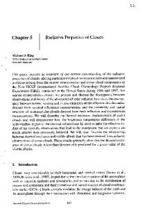
FIG. 1. Comparison of brightness temperature for IR channel 1 determined using the offline Fels–Schwarzkopf and Edwards–Slingo codes. The calculations assume a tropical atmosphere with water vapor amount scaled by a perturbation factor varying from 0.1 to 2.0. The intersection with the vertical line for a perturbation factor of 1.0 indicates the values for the tropical atmosphere.

agreement for clear-sky conditions. This indicates that the Roberts scheme has less impact on brightness temperatures than the CKD scheme. This was further demonstrated by implementing the CKD in the FS code, and the result from this implementation is shown as the longdash–dotted line.

a. Comparison of radiation codes We first compare the BTs determined using the two radiation codes for cloud-free conditions. Since the absorption in the IR window channel is dominated by the water vapor continuum, this comparison essentially shows the influence due to different water vapor continuum absorption schemes. The standard tropical atmosphere is used in the calculations. In order to consider the influence of water vapor amount over a wide range, the water vapor mixing ratio profile for the tropical atmosphere is multiplied by a factor varying from 0.1 to 2. The calculations assume a satellite view angle of 308 and are performed for the cases of water vapor line absorption only and line plus continuum absorption. The results are shown in Fig. 1. It is seen that the water vapor line absorption has a rather small influence on the BT. The radiation emitted at the surface is only reduced by about 2 K at the top of the atmosphere when the water vapor amount in the tropical atmosphere is increased by a factor of 2. The model results using the two radiation schemes (FS versus ES) for this case show a maximum difference of 0.5 K, with results from the ES code being higher. By contrast, the influence of the water vapor continuum absorption (Roberts versus CKD2.4) is much larger; the BT at the top of the tropical atmosphere decreases by about 8 K for doubled atmospheric water vapor amount. The BT difference between the two schemes, however, becomes small (dotted line and dot–dash line), and the two models show a good

b. Cloud IWC and optical properties A second set of offline calculations was performed to compare cloud IWC determined by two diagnostic schemes and their effect on the optical properties determined using the four ice optical parameterizations. As mentioned in the previous section, the cloud water content in GASP is determined by a temperature-dependent diagnostic scheme developed on the basis of several aircraft observations. Recently, Wang and Sassen (2002) presented a new relationship between IWC and temperature determined from 4 yr (1997–2000) of lidar–radar observations collected on the Southern Great Plains in Oklahoma, at the site of the cloud and radiation test bed of the Atmospheric Radiation Measurement (ARM) Program. They compared their results with aircraft observations taken over the midlatitudes and found that the IWC derived from the aircraft observations was higher than their lidar–radar observations for warm ice clouds (T . 2358C) and lower for cold ice clouds (T , 2408C). This finding suggests that the failure of GASP to produce enough cold BTs might be related to an underestimate of cloud ice water content in cold temperature regimes. Therefore a similar comparison is performed in this study. Figure 2 shows the relationship between ice water content and temperature determined using the operational scheme (GASP, solid curve) and that determined by the Wang and Sassen (2002) scheme (dotted curve).

2010

MONTHLY WEATHER REVIEW

FIG. 2. Cloud IWC as a function of cloud temperature. The symbols represent aircraft observations for midlatitude and tropical regions; the solid curve denotes the parameterization used by GASP based on aircraft observations, and the dotted curve shows the results determined using the Wang and Sassen (2002) parameterization based on lidar–radar measurements at the site of the ARM cloud and radiation test bed in Oklahoma.

The symbols represent aircraft observations collected from both midlatitude (Heymsfield and Platt 1984; Francis et al. 1994; Gultepe and Isaac 1997; Platt 1997) and tropical (McFarquhar and Heymsfield 1997) regions. It is clear that the difference between the two parameterization schemes is the same as that found by Wang and Sassen (2002). The observed IWCs from aircraft in both the midlatitudes and Tropics in the warm temperature region are systematically higher than the Wang and Sassen scheme. The reverse is true in the cold temperature region. Wang and Sassen claimed that the difference between the two sets of observations may be due to sampling different cloud types and the limitations of the in situ probes used in aircrafts. Such a large difference is really a matter of concern and should be investigated in terms of simultaneous lidar and aircraft observations. Here we test the two IWC parameterizations by using them to calculate the infrared (IR) absorption coefficients and compare the results with the observations from the lidar and IR radiometer (LIRAD) provided by Platt et al. (1984, 1987, 1998, 2002). This comparison may provide a partial validation for the two sets of independent IWC observations. The standard midlatitude summer atmosphere was used in these calculations. A cloud was assumed to lie between 200 and 230 mb, and four ice cloud optical property schemes were used. In order to compare these schemes in an appropriate manner the input to the schemes must be consistent, which can be difficult, as these schemes do not depend on the same input variables as outlined in the previous section. In general, the cloud IWC and effective sizes are essential variables and both are dependent on the cloud temperature as indicated in previous section. Therefore a simulation must include a simultaneous variation of cloud IWC and temperature. Using the IWC–temperature parameterizations satisfies this requirement. The simulations were therefore per-

VOLUME 132

formed for temperatures between 08 and 2758C using the two IWC parameterizations. It should be noted that the Wang and Sassen (2002) scheme is strictly only valid between 2208 and 2708C. We have extended beyond this range in order to get results over the wider range appropriate for real-world clouds. The temperature and ice water content were then used to calculate the effective sizes (G e , D , and req )and absorption coefficients. The observed absorption coefficients were taken from several field experiments described by Platt et al. (1984, 1987, 1998, 2002) who presented retrieved cirrus cloud absorption coefficients using LIRAD. These include 1) the Maritime Continent Thunderstorm Experiment (MCTEX; Platt et al. 2002) performed on the Tiwi Islands, about 120 km north of Darwin, Australia; 2) the ARM Pilot Radiation and Observation Experiment (PROBE) carried out in Kavieng, Papua New Guinea (Platt et al. 1998); 3) the winter of 1978 and summer of 1979/80 observations performed at Aspendale, Australia (Platt et al. 1987); and 4) observations for tropical thunderstorm anvils performed at Darwin (Platt et al. 1984). The detailed measurements and retrieval techniques can be found in the cited references. Figure 3 shows the absorption coefficients as a function of cloud temperature. The symbols show the observations derived by Platt et al. (1984, 1987, 1998, 2002) and the curves represent the theoretical results determined using the four optical property schemes. Figure 3a presents the modeled results using the Wang and Sassen (2002) IWC scheme, Fig. 3b the GASP IWC scheme, and Fig. 3c a hybrid (HYBRID) scheme; the Wang and Sassen scheme was used for T # 2508C, and GASP was used for T . 2508C. As can be seen the absorption coefficients from the observations show considerable scatter, but the variation with temperature is generally similar to that determined using the parameterized IWC. In the warm temperature region, the absorption coefficients observed in the midlatitudes (Aspendale) are systematically higher than those in the tropical region (PROBE) and the reverse is true at cold temperatures. The modeled values using the four optical property schemes with the IWC determined by the Wang and Sassen scheme are in reasonably good agreement with the observations for T , 2308C except for T , 2708C where all schemes underestimate the absorption coefficients compared with the observations in the Tropics. In the warm temperature region (T . 2308C) the model systematically underestimates the absorption. This discrepancy can be improved if the GASP IWC parameterization is used as shown in Fig. 3b, but with the result that the agreement in the cold temperature region becomes worse. It is also seen that the behavior of all four optical parameterizations are very similar except for the EC scheme at very cold temperature, which maintains roughly the same absorption coefficients for both IWC schemes. Thus the difference between the modeled and observed absorption coefficients is clearly due to the IWC rather than the optical property

AUGUST 2004

SUN AND RIKUS

2011

FIG. 4. Brightness temperature as a function of cloud ice water path determined using four ice optical parameterizations in conjunction with the HYBRID IWC scheme.

FIG. 3. Variations of absorption coefficient with cloud temperature. The symbols represent observations of the absorption coefficient determined by LIRAD, and the curves denote the theoretical results determined by four ice optical parameterizations. The modeled results are determined using (a) the Wang and Sassen scheme (b) the GASP scheme, and (c) a combination of Wang–Sassen for T , 2508C and GASP for T . 2508C.

schemes. If we believe the LIRAD-retrieved absorption coefficients are correct, then the results obtained here might mean that the lidar-retrieved IWCs in the warm temperature region and the aircraft observations in the

cold temperature region are both too low. These features may be explained by the fact that the IWC–temperature relationship of Wang and Sassen (2002) was derived from high clouds and may underestimate IWC in the warm temperature range, where middle-level ice clouds also exist. The aircraft instruments have a limitation in detecting small ice crystals in high clouds (Heymsfield and Platt 1984), and this may lead to underestimating IWC in the cold temperature range. If we accept this argument then it seems natural to consider the use of a hybrid scheme, that is, use the Wang and Sassen scheme for T , 2508C (the crossover point between the two curves in Fig. 2) and the GASP IWC scheme for T . 2508C. The modeled results determined using the HYBRID scheme are shown in Fig. 3c. It is seen from Fig. 2 that the observed IWCs for the cold clouds in the Tropics are somewhat higher than those in the midlatitudes. The observed cloud absorption coefficients for cold clouds in the Tropics as shown in Fig. 3 are a consequence of the higher IWCs and/or smaller crystal sizes in this region. This implies that the use of the GASP IWC parameterization based on aircraft observations for cold cirrus clouds underestimates IWCs in the midlatitudes, and if applied to the Tropics the results will be even worse. Therefore the use of the Wang and Sassen (2002) IWC scheme for cold cirrus clouds should certainly improve the model simulations in both regions; the scheme at least moves the model results in the right direction, and this will be further discussed in the following sections. Here we compare further the brightness temperatures determined using the four optical property schemes in conjunction with the HYBRID IWC scheme. The results are plotted as a function of IWP in Fig. 4. It is seen that the results determined using the Sun–Shine (1995) and Fu et al. (1998) schemes are in reasonably good agreement. The difference in BT between these schemes and the other two (EC and KEM) is significant and increases with IWP. The maximum difference in BT

2012

MONTHLY WEATHER REVIEW

FIG. 5. Impact of cloud particle scattering on BT calculations (results with scattering minus those without). The negative values mean that including the effect of scattering reduces the BT.

between Sun–Shine (1995) and the KEM scheme is about 10 K for an IWP of 100 g m 22 . This comparison indicates that the BT is sensitive to ice cloud optical properties and the selection of the ice cloud optical properties may be significant in improving model performance. The liquid water cloud optical properties and corresponding brightness temperatures determined using the two water cloud optical property schemes were also compared but no significant difference was found. Therefore the results are not presented here. In the following sections the results for the liquid water clouds were mostly derived using the Sun and Shine (1994) scheme unless stated otherwise. c. Effect of scattering We now investigate the effect of cloud particle scattering on the BT calculations. Similarly to the specifications used in the last section, we located a water cloud between 900 and 930 mb and an ice cloud between 200 and 230 mb. The calculations for the water cloud were performed using both the SS and HS schemes and those for the ice cloud were conducted using the Sun–Shine (1995) and Fu et al. (1998) schemes. The brightness temperature differences (the result with scattering minus that without scattering) are presented in Fig. 5. Negative values mean that including the effect of scattering in the calculation reduces the BT; the BTs are lower if the scattering effect is included in the calculations. The difference is 0.5–1.0 K depending on the value of LWP and the scheme used. The effect of scattering for the water cloud using the SS scheme is systematically larger than for the HS scheme (solid curve in Fig. 5). For the ice cloud, the difference due to the effect of scattering is generally less than that for water but still reaches about 0.5 K. The reason that the BT is reduced as a result of scattering is due to the fact that some photons

VOLUME 132

FIG. 6. Brightness temperature as a function of liquid fraction in a mixed-phase cloud. The cloud has a total water path of 100 g m 22 and is located between 400 and 500 mb of midlatitude summer atmosphere. Two satellite view angles are used in the calculations.

emitted at the surface travel upward and are scattered back to the ground. d. Cloud phase state The influence of changes in cloud phase state on BTs was investigated by placing a cloud between 400 and 500 mb with a total water path of 20 g m 22 equally distributed between these two levels. The ratio of liquid water to ice was varied from zero to unity. The optical properties were calculated using the Fu et al. (1998) scheme for ice and the HS scheme for water with the assumption that the ice particles and liquid drops uniformly mix together. The calculations were performed for the two satellite view angles of 08 and 458. The results are shown in Fig. 6. It is very clear that changes in cloud phase state have a significant influence on the BT. For a midlevel cloud situated at about 400 mb the brightness temperature for the nadir view can vary from 267 K if a cloud is purely ice to 252 K if it becomes entirely water. The difference of 15 K is reduced to about 10 K if the satellite view angle increases to 458. This result clearly indicates how important it is to correctly determine the cloud phase state in the BT calculations. 4. Comparison of modeled results with satellite measurements The GMS-5 satellite imagery is received in real time by the Bureau of Meteorology, accurately navigated, and then stored in the Man-computer Interactive Data Access System (McIDAS) database. These data are further averaged onto the model grid box for the comparison with the modeled results using the procedures described by Rikus (1997). For simplicity, the comparison in this paper is only presented for the GMS-5 domain

AUGUST 2004

SUN AND RIKUS

2013

FIG. 7. Comparison of BT in the infrared window channel determined using the validating system with the corresponding GMS-5 satellite imagery. The modeled results are valid for 0000 UTC 7 Jun and the GMS-5 imagery is for 2330 UTC 6 Jun. (a) The GMS-5 imagery, (b) the modeled results using the Fels–Schwarzkopf code, (c) the results determined using the Edwards–Slingo code, and (d) same as (c), but using the Wang and Sassen IWC scheme.

although the modeled results were derived using the global GASP domain. a. Comparison for two radiation codes First, the two radiation codes are compared. The control run was performed using the operational Fels– Schwarzkopf code together with the Clough et al. (1989) water vapor continuum and Sun–Shine optical property scheme and is referred to as FS–SS. The experimental run was conducted using the ES code with the same cloud optical property scheme, and this is referred to as ES–SS. The 24-h GASP model forecast fields valid at 0000 UTC on 7 June 2002 were used in the BT calculations. The closest satellite observations available are for 2330 UTC on 6 June. Figure 7 shows the results, where (a) is the satellite imagery, (b) is the result from the control run (FS–SS), and (c) shows the result from using the ES code (ES–SS). As can be seen, the model generally captures the major characteristics of the BT distribution pattern observed by the satellite. The midlatitude storm tracks in the Northern Hemisphere, the

subtropical frontal cloud system, the cold front system passing through the Tasman Sea and southern Australia, and the convective cloud cells over the Tropics are all clearly identified by model. Examining the detailed distributions, one can easily see that the modeled temperatures are not cold enough compared with satellite results, especially over the tropical region. The minimum BT observed by the satellite is 196 K but the corresponding value from the control run is only 220.2 K. The modeled mean temperature is also higher than the observed value. The result derived using the ES code is slightly better with a minimum temperature 2 K lower, but still not cold enough. b. Comparison for cloud amount and IWC The warm bias in the BT could be due to incorrect cloud amount, cloud height, and/or cloud microphysical properties. The modeled cloud height and amount are examined by plotting its vertical distribution. It is found that the model diagnoses cloud at levels as high as 75 hPa with appreciable cloud fraction. Figure 8 shows the

2014

MONTHLY WEATHER REVIEW

VOLUME 132

FIG. 8. Cloud fraction and ice water content (g m 23 ) at the seventh model level (about 100 hPa).

cloud fraction (left) and IWC (right) at the seventh model level, where pressures are about 100 hPa. It can be seen that the model diagnoses substantial cloud at this level. In fact, the cloud fraction at this level is too large compared with the satellite imagery (this will be further addressed below). The problem is thus more likely to be due to the model cloud IWC at these levels. One can see from the right panel of Fig. 8 that the cloud IWC is low. The values in the tropical region are uniformly less than 0.0002 g m 23 . Similar results are exhibited at adjacent levels. In the forward calculations these values are too small to enable the model clouds to produce any noticeable radiative effect even in overcast conditions. Consequently, clouds in these layers are optically too transparent to the radiation emitted from the underlying layers. As seen in section 2, the modeled IWC is lower in the cold temperature region than that from the ARM lidar– radar measurements. Therefore the underestimate of IWC at cold temperatures is most likely to be the source of the warm bias problem. To further test this hypothesis, we implemented the Wang and Sassen (2002) scheme in our model for temperatures less than 2508C and repeated the above calculations. Note that the Wang and Sassen scheme is strictly not valid for temperatures less than

FIG. 9. Same as Fig. 7d but using a modified high cloud fraction.

2708C. So a constant of 0.001 g m 23 is specified for T , 2708C. This value is about the same as that produced by the Wang and Sassen scheme at 2708C and it also results in a reasonable comparison between model and satellite. The results determined using the ES code together with this implementation are shown in Fig. 7d. It is seen that the BTs over the tropical region are colder than those shown in Fig. 7c. The minimum temperature

FIG. 10. Monthly mean (Jun and Dec 2002) frequency distributions of BTs for 58 bins derived from the GMS-5 imagery and the validation system. The two modeled results are derived using the same Fels– Schwarzkopf radiation scheme and Sun–Shine cloud optical properties scheme with different IWC schemes. ‘‘Orig’’ represents the modeled results determined using the original IWC and cloud schemes, and ‘‘modify’’ denotes those determined using Wang and Sassen’s scheme together with modified high cloud amount.

AUGUST 2004

2015

SUN AND RIKUS

FIG. 11. Monthly mean frequency difference (%) of BTs (model: GMS-5) for four ice-cloud optical property schemes.

drops to 209.5 K. This improvement demonstrates that the IWC determined by the Wang and Sassen scheme at cold temperatures may be closer to reality compared with the scheme based on aircraft observations over the tropical region. However the values are still not large enough to capture the observed minimum BTs. This is probably due to the fact that the Wang and Sassen scheme is an average for different-type high clouds while the deep convective clouds, which are usually responsible for the coldest observed BTs, have higher IWC than the average at a given temperature. Except for the difference in the minimum BTs the modeled BT field exhibits larger cloud areas in the tropical and subtropical regions than the satellite image. The mean brightness temperature over the entire region is also lower than the observed value. An investigation of the model moisture field has shown that the modeled relative humidity above 250 hPa over the tropical region is too large, even in the areas where no apparent clouds exist, leading to excess cloud fraction in these areas. The relatively large relative humidity in the upper troposphere is believed to be due to the use of a diagnostic cloud scheme. Newson (1998) has shown a similar problem existed in the ECMWF model when a diagnostic cloud scheme was used before 1995. After switching to a prognostic cloud scheme, the

monthly averaged relative humidity at 100 hPa was reduced from about 83% to 60% and the relative humidity between 300 and 700 hPa was increased, which is in much better agreement with observations. Newson claimed that this is due to the strong coupling of the clouds to the convection scheme so that the excess upper-level moisture is removed by precipitation into lower layers providing a source of water vapor on evaporation, and thereby increasing the relative humidity in these layers. While the above example provides a strong recommendation that a prognostic cloud scheme should be implemented into the GASP system in the longer term, the problem with the excess high-level cloud fraction derived by the diagnostic cloud scheme needs to be fixed for the time being. For this reason we modified the high cloud fraction parameterization by introducing the diagnosed IWC into the scheme, based on Randall’s (1995) simple cloud fraction parameterization. The cloud fraction in our model is determined by

1

2

RH 2 RHc f 5 , 100 2 RHc 2

(5)

where RH represents relative humidity, and RHc is

2016

MONTHLY WEATHER REVIEW

VOLUME 132

FIG. 12a. Verification results from the global NWP GASP model 7-day forecasts for the tropical region at 200 mb.

the critical relative humidity. For high clouds f is modified to f h 5 f [1 2 exp(2aIWC)],

(6)

where a is an empirical constant determined by tuning. Here, a 5 100 was found to give reasonable results. This expression indicates that when IWC 5 0, f h 5 0, and as IWC increases, f h increases. With this simple implementation, the excess high-level cloud fraction is effectively reduced. Figure 9 shows the BTs calculated using the ES code with the modification for high-level cloud fraction. It can be seen that the excess cloud area over the tropical and northern subtropical regions shown in Figs. 7b–d has been largely reduced. Another good sign obtained from this simple modification is that the mean temperature for the whole domain is also in better agreement with the satellite observation. The results shown above are only obtained from one case. In order to examine the impact of the modifications

in different cases, the validation system has been run for two complete months, June and December 2002, using the operational FS radiation code in conjunction with Sun–Shine (1994, 1995) cloud optical properties. The results are compared with the satellite measurements. All modeled results were determined using the GASP 24-h forecast fields valid at 0000 UTC and the satellite images for 2330 UTC. Figure 10 shows a frequency distribution of brightness temperature in 58C bins for the GMS-5 domain. They are averaged over the 30 days for each month. The key ‘‘orig’’ indicates the modeled results determined using the original IWC and cloud schemes, and ‘‘modify’’ represents those determined using the HYBRID IWC scheme together with the modified high cloud amount. It is seen that with the original IWC scheme the model does not produce the distribution of monthly mean BTs below 220 K in either month. In June, the frequency of BTs between 235 and 275 K from the control run is higher than that from

AUGUST 2004

SUN AND RIKUS

2017

FIG. 12b. Same as in Fig. 12a but for the Northern Hemisphere annulus at 100 mb.

GMS-5, and the reverse is true for BTs greater than 285 K. These errors have been noticeably reduced by the HYBRID IWC scheme and modified high cloud scheme although in two BT bins (280 and 290 K) the modified results become worse. The frequency distribution in December is broader than that in June because of a larger amount of convective activities, and hence greater cloudiness over the month. The difference between the two experiments in December is not as large as that in June, but it is still clear that the modified scheme produces results that are better than the original ones, especially in the warm temperature bins. c. Comparison for cloud optical properties Next we examine the effects of cloud optical properties in the validation system. As mentioned before, the two water cloud optical property schemes do not make sig-

nificant differences to the BT comparison, and therefore we only compare the results determined using the four ice cloud optical property schemes in conjunction with the Sun–Shine (1994) water cloud scheme. In these calculations the HYBRID IWC scheme and the high-level cloud fraction modification are used. The monthly mean frequency differences (model 2 GMS-5) in June and December 2002 determined from these calculations are plotted in Fig. 11. It is seen from the frequency difference distributions that the model results using the four ice cloud optical property schemes are generally compatible. The negative values for T , 215 K and 240 , T , 280 K mean that the number of model BTs in these ranges is less than that of the satellite and vice versa in the other regions. Although the difference between these schemes is not significant, the results over the two months determined from the Sun–Shine (1994, 1995) and Fu et al. (1998) schemes are generally better than the others com-

2018

MONTHLY WEATHER REVIEW

VOLUME 132

FIG. 12c. Same as in Fig. 12a but for the Southern Hemisphere annulus at 850 mb.

pared with the satellite. It should be pointed out that these results are only true in the infrared window channel. The behavior of these schemes in the visible channels may be very different and needs to be carefully examined. This will be our next step, as part of the inclusion of the visible channels in the validation system. It must be also emphasized that the results from this study are highly system dependent and should only be regarded as a general guide. 5. Impact on GASP The major finding from the above investigations is that the use of the new IWC scheme of Wang and Sassen (2002) in the cold temperature region reduces the warm bias for cloud-top temperature in the validating system. The natural question one may ask is, How does this scheme affect the performance of the NWP GASP mod-

el? To answer this question, the scheme has been implemented in the T239/L29 version of GASP and its impact on the NWP forecast results tested. The operational FS radiation code was used in the tests. The only changes relative to the operational forecast run are the use of the Wang and Sassen IWC when the cloud temperature is less than 2508C and the ice water content correction applied to the diagnostic high-level cloud amounts. We found that the new scheme has a positive impact on the model forecast over the 21 cases of selfverified forecasts from 18 August to 7 September 2002 that were performed. During this period GASP has a cold bias at almost all levels. Using the HYBRID IWC scheme and modified high-level cloud amount reduces these cold biases and associated rms errors. Figure 12 shows the verification results for (a) the tropical region at 200 mb (b) the Northern Hemisphere annulus at 100 mb, and (c) the Southern Hemisphere annulus at 850

AUGUST 2004

2019

SUN AND RIKUS

mb. The solid curve represents the results determined by the operational run, and the dashed curves denote those from the experiment run. As can be seen, model biases are improved. This positive impact can also be seen in most other regions and levels, but the most significant improvement occurs over the Tropics. This result is consistent with the BT comparisons. The radiative effect of upper-level cloud on the system is dominated by the longwave greenhouse warming. If a modeled cloud at upper levels is not optically thick enough then the model warm bias in BT at the top of the atmosphere and cold bias below the cloud layer will occur simultaneously as a result of enhanced outgoing longwave radiation. 6. Summary The new BT code together with several cloud optical property schemes are tested using the Bureau of Meteorology’s cloud validation system. The purpose of this work is to investigate possible reasons for the persistent warm bias in the BT simulations in the bureau’s GASP system. Some offline calculations were performed to examine the effects on the BT simulation due to the use of different cloud optical property schemes, cloud scattering, and cloud phase state. The results show that the optical property schemes for the water cloud do not cause significant differences in the BT calculations but those for ice cloud do. Our test results show that of the two radiation codes the modified Edwards and Slingo (1996) code generally produces a better BT field compared to the satellite observations. For the ice cloud optical property schemes, it is hard to get a solid conclusion as to which scheme is best because of the system dependence. The modeled results using these schemes are generally compatible. The problem of the warm bias in the BT simulations by GASP is mainly due to an underestimate of IWC at cold temperatures as determined by the temperaturedependent scheme used in the GASP model. This is supported by the ARM lidar–radar measurements that show higher IWC in the cold temperature regions than aircraft observations. Although the ARM IWCs were observed at midlatitudes, the application of these values to the calculations of the cloud absorption coefficients at cold temperatures leads to a better comparison with the observations determined by LIRAD than using the aircraft-based IWCs for both the midlatitudes and Tropics. This may justify its application in the tropical region. More importantly, implementation of the ARM IWCs in the cold temperature regions has led to significant improvement in the BT calculations, and the use of this scheme in the GASP system also improves the model forecast performance. Although the ARM IWCs in the cold temperatures are useful in improving model simulations, the values in the warm temperature region seem too low compared with the aircraft observations. The cloud absorption co-

efficients determined using the ARM IWCs are also substantially underestimated compared with the observations determined by LIRAD. This discrepancy may need to be investigated with simultaneous LIRAD and aircraft observations. The study also reveals the limitations of the diagnostic cloud scheme operating in the upper troposphere in our GASP system, which may motivate an implementation of a prognostic cloud scheme in the near future. Acknowledgments. The authors would like to acknowledge the anonymous reviewers. Their comments and suggestions lead to improving the paper quality. REFERENCES Bourke, W. P., T. J. Hart, P. J. Steinle, R. S. Seaman, G. Embery, M. J. Naughton, and L. J. Rikus, 1995: Evolution of the Bureau of Meteorology’s global data assimilation and prediction system. Part II: Resolution enhancements and case studies. Aust. Meteor. Mag., 44, 19–40. Clough, S. A., F. X. Kneeizys, and R. W. Davies, 1989: Line shape and the water vapor continuum. Atmos. Res., 23, 229–241. Ebert, E. E., and J. A. Curry, 1992: A parametrization of ice cloud optical properties for climate models. J. Geophys. Res., 97, 3831–3836. Edwards, D. P., 1992: GENLN2: A general line-by-line atmospheric transmittance and radiance model. NCAR Tech. Note TN3671STR, National Center for Atmospheric Research, Boulder, CO, 147 pp. Edwards, J. M., and A. Slingo, 1996: Studies with a flexible new radiation code. I, Choosing a configuration for a large-scale model. Quart. J. Roy. Meteor. Soc., 122, 689–719. Francis, P. N., A. Jones, R. W. Saunders, K. P. Shine, A. Slingo, and Z. Sun, 1994: An observational and theoretical study of the radiative properties of cirrus: Some results from ICE’89. Quart. J. Roy. Meteor. Soc., 120, 809–848. Fu, Q., P. Yang, and W. B. Sun, 1998: An accurate parametrization of infrared radiation properties of cirrus clouds for climate models. J. Climate, 11, 2223–2237. Gultepe, I., and G. A. Isaac, 1997: Liquid water content and temperature relationship from aircraft observations and its application to GCMS. J. Climate, 10, 446–452. Heymsfield, A. J., 1975: Cirrus uncinus generating cells and the evolution of cirriform clouds. Part I: Aircraft observations of the growth of the ice phase. J. Atmos. Sci., 32, 799–808. ——, and C. M. R. Platt, 1984: A parameterization of the particle size spectrum of ice clouds in terms of the ambient temperature and the ice water content. J. Atmos. Sci., 41, 846–855. Hu, Y. X., and K. Stamnes, 1993: An accurate parameterization of the radiative properties of water clouds suitable for use in climate models. J. Climate, 6, 728–742. Kristjansson, J. M., J. M. Edwards, and D. L. Mitchell, 1999: A new parameterization scheme for the optical properties of ice crystals for use in general circulation models of the atmosphere. Phys. Chem. Earth, 24B, 231–236. Lemus L., L. Rikus, and C. R. M. Platt, 1997: Global cloud liquid water path simulations. J. Climate, 10, 52–64. Martin, G. M., D. W. Johnson, and A. Spice, 1994: The measurement and parameterization of effective radius of droplets in warm stratocumulus clouds. J. Atmos. Sci., 51, 1823–1842. McFarquhar, G. M., and A. J. Heymsfield, 1997: Parameterization of tropical cirrus ice crystal size distributions and implications for radiative transfer: Results from CEPEX. J. Atmos. Sci., 54, 2187– 2200. Mitchell, D. L., Y. Liu, and A. Macke, 1996: Modeling cirrus clouds.

2020

MONTHLY WEATHER REVIEW

Part II: Treatment of radiative properties. J. Atmos. Sci., 53, 2967–2988. Mlawer, E. J., S. J. Taubman, P. D. Brown, M. J. Iacono, and S. A. Clough, 1997: Radiative transfer for inhomogeneous atmospheres: RRTM, a validated correlated-k model for the longwave. J. Geophys. Res., 102, 16 663–16 682. Morcrette, J. J., 2002: The surface downward longwave radiation in the ECMWF forecast system. J. Climate, 15, 1875–1892. Moss, S. J., and D. W. Johnson, 1994: Aircraft measurements to validate and improve numerical model parameterizations of ice to water ratios in clouds. Atmos. Res., 34, 1–25. Newson, R., 1998: Results of the WCRP first international conference on reanalyses. GEWEX News, Vol. 8, No. 1, International GEWEX Project Office, Silver Spring, MD, 3–8. Platt, C. M. R., 1997: A parameterization of the visible extinction coefficient of ice clouds in terms of the ice/water content. J. Atmos. Sci., 54, 2083–2098. ——, A. C. Diliey, J. C. Scott, I. J. Barton, and G. T. Stephens, 1984: Remote sounding of high clouds. V: Infared properties and structures of tropical thunderstorm anvils. J. Appl. Meteor., 23, 1296– 1308. ——, J. C. Scott, and A. C. Diliey, 1987: Remote sounding of high clouds. Part VI: Optical properties of midlatitude and tropical cirrus. J. Atmos. Sci., 44, 729–747. ——, S. A. Young, P. J. Manson, G. R. Patterson, S. C. Marsden, and R. T. Austin, 1998: The optical properties of equatorial cirrus from observations in the ARM pilot radiation observation experiment. J. Atmos. Sci., 54, 1977–1996. ——, ——, R. T. Austin, G. R. Patterson, D. L. Mitchell, and S. D. Miller, 2002: LIDAR observations of tropical cirrus clouds in MCTEX. Part I: Optical properties and detection of small particles in cold cirrus. J. Atmos. Sci., 59, 3145–3162. Randall, D. A., 1995: Parameterizing fractional cloudiness produced by cumulus detrainment. WMO Tech. Doc. 713, 1–16. Rikus, L., 1997: Application of a scheme for validating cloud in an operational global NWP model. Mon. Wea. Rev., 125, 1615– 1637. ——, and M. Salby, 2000: Validation of the temporal variation of cloud imagery derived from a global NWP model. Proc. 11th

VOLUME 132

BMRC Modelling Workshop, Melbourne, Victoria, Australia, BMRC, 157–160. Roberts, E., J. E. A. Selby, and L. M. Biberman, 1976: Infrared continuum absorption by atmospheric water vapour in the 8–12 mm window. Appl. Opt., 15, 2085–2090. Rossow, W., and R. A. Schiffer, 1991: ISCCP cloud data products. Bull. Amer. Meteor. Soc., 72, 2–20. Rothman, L. S., and Coauthors, 1998: The HITRAN molecular spectroscopic database and HAWKS (HITRAN Atmospheric Workstation): 1996 editions. J. Quant. Spectrosc. Radiat. Transfer, 60, 665–710. Rotstayn, L., 1997: A physical based scheme for the treatment of stratiform clouds and precipitation in large-scale models. I: Description and evaluation of the microphysical processes. Quart. J. Roy. Meteor. Soc., 123, 1227–1282. Schwarzkopf, M. D., and S. B. Fels, 1991: The simplified exchange method revisited: An accurate, rapid method for computation of infrared cooling rates and fluxes. J. Geophys. Res., 96, 9075– 9096. Stephens, G. L., and C. M. R. Platt, 1987: Aircraft observations of the radiative and microphysical properties of stratocumulus and cumulus cloud fields. J. Climate Appl. Meteor., 26, 1243–1269. Sun, Z., and K. P. Shine, 1994: Studies of the radiative properties of ice and mixed phase clouds. Quart. J. Roy. Meteor. Soc., 120, 111–137. ——, and ——, 1995: The potential climatic importance of mixedphase clouds. J. Climate, 8, 1874–1888. ——, and L. Rikus, 1999a: Improved application of ESFT to inhomogeneous atmosphere. J. Geophys. Res., 104, 6291–6303. ——, and ——, 1999b: Parameterization of effective radius of cirrus clouds and its verification against observations. Quart. J. Roy. Meteor. Soc., 125, 3037–3056. ——, and D. Pethick, 2002: Comparison between observed and modelled radiative properties stratocumulus clouds. Quart. J. Roy. Meteor. Soc., 128, 2691–2712. Wang, Z., and K. Sassen, 2002: Cirrus cloud microphysical property retrieval using lidar and radar measurements. Part II: Midlatitude cirrus microphysical and radiative properties. J. Atmos. Sci., 59, 2291–2302.