free filtering is used for cycle estimation of widelane ... the advantage of code/carrier divergence-free filtering .... LAMBDA bootstrap decorrelation method [3].
Validation of Autonomous Airborne Refueling Algorithms Using Flight Test Data Samer Khanafseh and Boris Pervan, Illinois Institute of Technology, Chicago, IL Jennifer Gautier and Per Enge, Stanford University, Stanford, CA Glenn Colby, Naval Air Warfare Center, Patuxent River, MD ABSTRACT Successful Autonomous Airborne Refueling (AAR) has the potential to increase the mission range of unmanned aerial vehicles (UAVs). AAR requires that the position of the receiving aircraft relative to the tanker be known very accurately and in real time. In addition, to ensure safety and operational usefulness, the navigation architecture must provide high levels of integrity, continuity, and availability. We begin this paper with a reminder of the latest proposed Shipboard Relative GPS (SRGPS) navigation architecture, which we exploit as a preliminary basis for AAR navigation. The AAR mission is different from SRGPS because of the potentially severe sky blockage introduced by the tanker, which degrades the positioning accuracy. In this work, we provide a high accuracy and high fidelity dynamic blockage model for a KC-135 tanker. AAR flight tests were conducted to obtain time-tagged GPS and INS data that were processed offline in order to validate the KC-135 blockage model and the AAR navigation algorithms. Finally, a worldwide global AAR availability analysis is presented for a grid of 10 degrees in latitude and longitude.
INTRODUCTION Unmanned Air Vehicles (UAVs) have recently generated great interest because of their potential to perform hazardous missions without endangering the lives of pilots and crews. In order to extend the mission range of these vehicles, it has been proposed that they should be refuelable in-air using currently available tanker aircraft. Since UAVs are unmanned, such refueling missions must take place autonomously. The position of the UAV relative to the tanker must therefore be known very accurately and in real time. In addition, to ensure safety and operational usefulness, the navigation architecture must provide high levels of integrity, continuity and availability. Overall the navigation requirements for autonomous air refueling (AAR) are similar to those for the shipboard landing of aircraft. In this paper, we first introduce the latest proposed Shipboard Relative GPS (SRGPS) navigation architecture [1], which uses Carrier
phase Differential GPS (CDGPS), and we exploit it as a preliminary basis for AAR navigation. However, the AAR mission is different from SRGPS because of the potentially severe sky blockage introduced by the tanker (here a KC-135 tanker) (Figure 1). In previous work [2], we provided an approximate blockage model and conducted an availability analysis for six different sites. Here, the availability analysis is expanded worldwide using a grid of 10 degrees in latitude and longitude. To validate the AAR algorithms, a flight test was conducted in which a Lear jet was used to emulate the UAV. In the previous work, when the flight test data were used to validate the previous blockage model, notable discrepancies with the measurements were noticed. It was concluded that these discrepancies were caused either by the approximations in this earlier blockage model or by the Precision GPS (PGPS) tanker-to-Lear relative vector that had been provided along with the raw flight test data. To study these two possible causes of mismatch, we provide a high accuracy and high fidelity blockage model and investigate the accuracy of the relative vector history that was provided by generating a ‘truth’ vector. The truth vector is generated using the prototype AAR PGPS relative navigation algorithms applied to the raw flight test data. Finally, the new KC-135 blockage model and the SRGPS based algorithms are validated using the raw flight test data.
Figure 1: A picture taken at pre-contact position showing the amount of sky blockage introduced by a KC-135 tanker.
The AAR navigation algorithms, which are based on the SRGPS architecture, provide robust CDGPS performance by combining the complementary benefits of geometryfree filtering and geometric redundancy. Specifically, when the aircraft is far from the tanker, inside or outside the service volume (i.e., the region where tanker reference GPS measurements are available to the UAV), geometryfree filtering is used for cycle estimation of widelane integers (Figure 2). For dual frequency implementations, the advantage of code/carrier divergence-free filtering prior to the service volume entry can be especially significant because long filter durations are possible. The use of geometric redundancy for cycle resolution is restricted to the service volume, where the aircraft has access to the tanker reference measurements, and is more robust to ionospheric and tropospheric decorrelation as the distance between the aircraft and the tanker is small. Therefore, only when the aircraft is near the tanker, can carrier phase geometric-redundancy be safely exploited for cycle estimation of any remaining wide-lane integers and, if needed, L1 and L2 integers. However, the AAR mission is different from any other mission because of the severe blockage that is introduced by the tanker, which reduces the number of visible GPS satellites and hence degrades the positioning accuracy (Figure 1). In order to predict and hence limit the effect of the satellite blockages, the AAR mission can be simulated using, the known GPS constellation at the time of the mission, the heading of the tanker and the blockage model (Figure 3). Here, a detailed blockage model is developed utilizing the full 3D shape of a KC-135 tanker. Using this simulation, the tanker can estimate which satellites will be blocked during the mission and the resulting positioning accuracy degradation and can potentially decide to change the
heading in order to avoid satellite blockages. Once the UAV enters the service volume, the tanker has access to the UAV measurements and is able to simulate the AAR mission and to decide whether to abort, continue or modify the refueling path. If the positioning accuracy and integrity requirements are met, the UAV’s will move to the observation position (tanker lead formation), where the UAV’s are just off the wing of the tanker and in the clear sky (Figure 4). At that point the carrier phase geometric-redundancy can be safely exploited for cycle estimation of L1 and L2 integers. From this point and on, CDGPS positioning of the UAV with respect to the tanker can be implemented. Again, when the UAV moves to the contact position (below the belly of the tanker), some satellites will be blocked (Figure 5), but the positioning accuracy is ensured to remain within the required limit (because the simulation has already taken these blockages into account).
Figure 2: Conceptual drawing shows both aircraft pre-filtering widelane integers before the UAV inters the service volume.
Figure 3: The tanker will have access to the UAV measurements and will be able to simulate the mission when the UAV enters the service volume.
In a first section of this work, in order to analyze the performance of the prescribed architecture, an availability analysis is conducted. Using this architecture and the blockage model that was developed in previous work [2], a global availability of AAR is performed. This phase of the study is designed to predict the visibility of GPS satellites by the Joint Unmanned Combat Aircraft System (J-UCAS) tanking aircraft (KC-135), and the resulting availability of a precise navigation solution, as a function of location on the globe, and direction of flight; this latter variable is necessary because the shading of the tanking aircraft is not symmetrical with respect to the GPS satellite constellation but depends on the direction of flight.
Figure 4: Geometric redundancy is applied when the UAV is in the observation position and very close to the tanker (in clear sky).
Figure 5: Some satellites will be blocked when the UAV goes below the tanker belly.
In the following sections, we evaluate the blockage model as well as the AAR architecture using data from AAR flight tests that were conducted in September 2004, in Niagara Falls. During these tests, a Lear jet was used to replace and simulate the UAV. We obtained time-tagged GPS and INS data that were processed using offline GPS algorithms. To analyze the actual flight test data, the fact that both aircraft are moving continuously must be accounted for. Therefore, a new dynamic version of the blockage model was constructed. The dynamic blockage model uses the relative position vector and the attitude information from both aircraft to create the tanker masking shadow and find the blocked satellites. In addition, to investigate the accuracy of the tanker-to-Lear relative vector history, a ‘truth’ vector is generated by applying the prototype AAR PGPS relative navigation algorithms to the raw flight test data. Finally, the AAR algorithm validation is obtained by comparison between the satellites predicted blocked as estimated using the dynamic model with the satellites actually blocked as indicated by drops in signal quality and phase lock losses of the measurements.
widelane and L1 and L2 integers which meet a 10-8 constraint for probability of incorrect fix using the LAMBDA bootstrap decorrelation method [3]. After the integer fixing process, the position of the receiver aircraft can be estimated with optimal accuracy.
GLOBAL AVAILABILITY SIMULATIONS
The vertical component of the position estimate standard deviation (σV) is calculated and used to generate the VPL. The VPL is calculated by multiplying σV by the integrity risk multiplier corresponding to the integrity risk requirement (5.33 in the case of 10-7 integrity risk). For the simulations presented in this paper, it was assumed that the raw code (pseudorange) single difference ranging error standard deviation is 30 cm and that the single difference carrier ranging error standard deviation is 1 cm. In addition, the results presented here assume a first order Gauss-Markov measurement error model with a time constant of one minute. We consider a 27 satellite constellation [4] (24 nominal + 3 operational spares) and an elevation mask of 3 degrees. The refueling boom is assumed to be in the nominal position, with 6 ft extension, 0 deg azimuth, and 30 deg elevation. As illustrated in Figure 6, the front GPS antenna location—upon which the blockage model is based—is 60 inches aft of the refueling point.
In this work, availability is defined as the percentage of time that the Vertical Protection Level (VPL) is smaller than a Vertical Alert Limit (VAL) of 1.1 m. The VPL is a function of the integrity risk (10-7 for SRGPS), the satellite geometry, and the precision of the GPS measurements. The VPL is generated by covariance analysis of the notional AAR navigation architecture mentioned above. In this analysis, a maximum prefiltering period of 30 minutes is assumed to generate floating estimates of the widelane cycle ambiguities. In addition, geometric redundancy is exploited to fix the
In order to study the effect of the geographic location of the airborne refueling mission on availability, a grid map of AAR locations is used Figure 7. The selected locations are distributed on a grid of 10 deg increments in longitude and latitude. In addition, to improve the resolution in the mid-latitude regions, a finer grid size of 5 degrees in latitude is implemented between latitudes of -40 and 40 deg. This simulation is executed for one sidereal day (23 hours and 56 minutes) and for flight headings from 0 to 345 degrees in 15 degree increments. In this study, availability is quantified by the number and
length of observed navigation outages. An outage is identified at the instant the VPL value becomes greater than the proposed 1.1 m VAL. Outage maps were constructed for each flight heading and combined in a single composite plot in Figure 8. The availability results with respect to the heading are shown in Table 1. In this map, we distinguish three levels of outage durations; outages of one minute duration (green areas), outages greater than one minute but less that 10 minutes (yellow areas), and outages of more than 10 minute duration (red areas). In addition, the total number of outages that occurred for all headings are presented at each point in the format (a/b/c), where a, b and c are the number of headings that encountered an outage at that geographic point for respectively one minute, more than one but less than ten minutes, and more than ten minutes. In addition, the average availability and worst availability values are
calculated using the equations below and the results are given on the top corners of the map and in Table 1: m
Average Availability =
m ⋅ T − ∑ Tout ,i i =1
m ⋅T
⎛ T − Tout ,i Worst Availability = min im=1 ⎜⎜ ⎝ T
⎞ ⎟⎟ ⎠
where, m: total number of grid points, T: is the number of minutes per sidereal day (1336), Tout,i: is the total outage duration for grid point i.
90° N
°
45 N
180 0° ° W
135° W
90° W
45° W
0°
45° E
90° E
135° E
180° E
45° S
90° S
Figure 6: The GPS antenna point used in this study and the corresponding blockage az-el plot.
Figure 7: World map showing the simulation grid points.
Figure 8: Composite map of all headings showing the outages at the grid points.
Table 1: Global availability results (average and worst availability) for different heading angles.
k k ΔφurL xur + Δτ ur + λ L1 N Lk1 + ν φL1 1 = −e T
k k ΔφurL xur + Δτ ur + λ L 2 N Lk 2 + ν φL 2 2 = −e T
Heading (deg)
Average Avail. %
Worst Avail. %
0 75 90 105 180 195 225 255 270 285 315 345 Else
99.9995 99.9979 99.9917 99.9979 99.9995 99.9995 99.9985 99.9902 99.9835 99.9902 99.9985 99.9995 100.000
99.9304 99.7911 99.4429 99.7911 99.9304 99.9304 99.7911 99.5822 99.5822 99.5822 99.7911 99.9304 100.000
Note that the 1 minute outages are not accounted for in Tout because it was assumed that an integrated INS system would be capable of bridging outages of up to one minute in duration. Figure 8 shows that there is not a single incident of an outage lasting more than 10 minutes for any grid point and any heading. The worst availability for any grid point and heading is 99.16%. However, the average availability over all headings and all grid points is 99.9978. These results are encouraging because they show that there is always a time/heading combination that allows the UCAV to be refueled autonomously all over the globe. TRUTH POSITION VECTOR GENERATION
k k k ΔφurL 1 − Δρ urL1 = λ L1 N L1 + ν CMC L1
(1)
(2)
k k k ΔφurL 2 − Δρ urL 2 = λ L 2 N L 2 + ν CMC L 2
where, k k ΔφurL1 , ΔφurL2 : user-reference single difference
L1/L2 carrier range for satellite k
Δρ
k urL1
, Δρ urL2 : user-reference single difference k
L1/L2 pseudo-range for satellite k e: line of sight vector for satellite k xur: relative position vector between the user and the reference Δτ ur : differential receiver clock bias
λ L1 : L1 carrier wavelength N Lk1 : L1 integer cycle ambiguity for satellite k
ν
: measurement noise
Then, the forward and backward L1/L2 solutions are combined to produce the optimal estimate of the floating cycle ambiguities as shown in Equation 3 [5],
(
−1 −1 Pˆn = PnF + PnB+1
(
)
−1
−1 −1 Nˆ n = Pˆn ⋅ PnF ⋅ N nF + PnB+1 ⋅ N nB+1
)
(3)
where,
As concluded in previous work [2], one of the possible reasons for the remaining discrepancies between the blockage model predictions and the receiver measurements is that the initial PGPS relative position between the tanker and Lear vector history is not accurate enough. This initial vector (referred to here as the ‘TSPI’ vector) was generated post-flight using a commercially available measurement processing software. To investigate the accuracy of this vector (and the resulting impact on the blockage model validation), a ‘truth’ vector history is generated using the raw flight test data. The truth trajectory is generated using prototype AAR PGPS relative navigation algorithms developed at the Illinois Institute of Technology (IIT).
Pˆn : covariance matrix of the smoothed integers at the
The truth vector generation algorithm uses a forwardbackward smoothing technique to optimize the accuracy of the GPS integer cycle ambiguity estimates. In both the forward and the backward cases, satellite geometric redundancy (Equation 1) and geometry free filtering (Equation 2) are used to estimate floating L1/L2 cycle ambiguities.
If possible, the smoothed integers are rounded using the LAMBDA bootstrap decorrelation method with 0.99 threshold on the probability of correct fix [3]. Finally, kinematic carrier phase positioning is implemented to estimate the truth vector,
nth epoch
PnF : covariance matrix of the forward solution at the nth epoch
PnB+1 : covariance matrix of the backward solution at the (n+1)th epoch
Nˆ n : smoothed integers at the nth epoch
N nF : forward solution of the integers at the nth epoch
N nB+1 : backward solution of the integers at the (n+1)th epoch
k kT ˆ ΔφurL xur + Δτ ur + ν (φ − N )L1 1 − λ L1 N L1 = −e
Δφ
k urL 2
T − λ L 2 Nˆ L 2 = −e k xur + Δτ ur + ν (φ − N )L 2
(4)
Figure 9: Antenna locations on the Lear jet airplane.
Figure 10: Estimated differential clock bias versus time.
Figure 11: Truth Vector Estimation for the IIT Static Antenna Test.
Figure 12: One Sigma Covariance Envelope and Measured Position Estimate Error for the IIT Static Antenna Test.
The Lear jet that was used in the flight test was equipped with two antennas; the front which is connected to NovAtel OEM4 receiver, and the back which is connected to Rockwell EMAGR receiver (Figure 9) and the tanker has only one antenna which is connected to both OEM3 and EMAGR receivers. Preliminary results show large differential receiver clock biases between the Lear and the tanker for OEM4 data (Figure 10). These biases will have a great effect on the single difference position estimation because they indicate a time misalignment on the order of milliseconds (meters in the position domain) between the tanker and the Lear measurements. Therefore, a time alignment procedure is needed before estimating the position or the integer ambiguities. Instead of the two-step process of estimating the clock biases then adding the alignment correction to the measurements, an implicit time alignment strategy is followed [6]. With this method, the time alignment is implemented directly during the integer and position estimation. The observation matrix
components corresponding to the differential clock bias are not set to ones but are modified by the Doppler of each satellite. In addition to the time alignment correction, inter-frequency biases are also observed in the measurements and are added to the estimated states as follows,
( ) + (1 − φ& )Δτ
k kT ΔφurL xur + 1 − φ&rLk 1 Δτ ur + λ L1 N Lk1 + ν φL1 1 = −e k k ΔφurL xur 2 = −e T
k rL 2
ur
+ b f + λ L 2 N Lk 2 + ν φL 2
where,
φ&rLk 1 , φ&rLk 2 : bf
L1/L2 Doppler of the kth satellite for the reference receiver : inter-frequency bias
These algorithms are first validated using data from two static antennas at IIT. Figure 11 shows the enhanced
performance in position estimation using the forwardbackward fixed integers as compared to the forward floating solution. In this analysis, a three-minute update period (to ensure whitening of time-correlated multipath errors) is used for the cycle ambiguity estimation filter, and a one-second sample period is used for carrier phase positioning. Comparison of the estimated vector with the known true value of the baseline distance between the two antennas shows that the relative vector is estimated with less than 5 mm error. The accuracy of the result matches the predicted standard deviation of the position estimate error, which is approximately 1 cm. The estimate-error results for this test case are shown in Figure 12. Unlike the test case above, the relative vector between the tanker and Lear is changing continuously during the AAR flight test. In addition, because the Lear was closely following the tanker, higher multipath errors are expected and many satellite outages (blockages) are observed. These factors impact both the floating cycle ambiguity estimation accuracy and the integer fixing capability. Figure 13 shows the difference between the original TSPI vector and the newly estimated truth vector in the north direction. The predicted estimate error standard deviation envelope (one sigma) of the new position vector is also shown. It is observed that due to the frequent blockages at the Lear, the carrier phase integers could not always be fixed, even if the probability of correct fix was relaxed to 0.99. This can be explained by the many outages happening within the three-minute measurement update. However, using an update period lower than 3 minutes is not recommended, because the receivers' code measurements were smoothed with a 100 sec time
Figure 13: AAR truth vector estimation using IIT code with fixing integers (if possible) for OEM4 receiver.
constant, which in turn causes significant correlation between measurements. In order to validate the generated truth vector independently, a separate truth vector estimation for the back antenna was generated. The back receiver being different from the front one, time alignment issues were considered again. In this case, it is found that the time alignment step is not needed, which makes the estimation of both vectors independent and enables validation of the vector generation algorithms. The generated truth vector from the back antenna can be compared to the front one after applying the lever arm correction. Figure 14 shows the difference between the translated result for the back antenna and the TSPI vector in the north direction. As is evident in the comparison of Figures 13 and 14, both the front and the back vectors match when integers can be fixed, which validates again the vector generation algorithm. In addition, a new vector can be constructed by fusing the results from both antennas when the integers could be fixed. Figure 15 shows a sample result of the fused position vector. It can be seen that even when fusing both the front and the translated back position vectors, there are still occurrences where the position accuracy is worse than 27 cm. The accuracy is degraded because the integers could not be fixed at those specific times. The intermittent integer fixing can be justified by the significant satellite blockages occurring at these instances. This is of no surprise because the flight test mission planning aimed at selecting worst case time and tanker heading with respect to satellite blockages [2].
Figure 14: AAR truth vector estimation for the back antenna (EMAGR receiver) after applying the lever arm correction.
Figure 15: Fused truth vector of both the front and back antenna solutions.
Figure 16: 3D Dynamic Blockage Model algorithm Structure.
BLOCKAGE MODEL
the 3D tanker mesh. Therefore, a 2D snapshot can be easily converted to azimuth and elevation angles using trigonometry, which OpenGL efficiently provides. In short, OpenGL is analogous to a virtual photographic studio with a camera, different types of lenses, a projector, and a projector screen (where the final 2D snapshot will be presented). For the AAR blockage application, the camera is fixed at the Lear’s GPS antenna location and oriented toward the tanker. The lens is defined by the desired view field, which includes the view angle of the scene, and nearest and farthest distances the camera is required to capture. The near-camera face of the view field also defines the coordinates of the corners of the rectangle that will act as a projection screen (as illustrated in Figure 17). These view field parameters are calculated at each epoch to ensure the best resolution performance and that all parts of the airplane are captured. Once the scene is prepared in this way, OpenGL is used to generate a 2D pixel-based matrix that represents the 2D projection of the tanker on the screen. Because the real dimensions of the projection screen are already known, the pixel matrix can be easily converted to real dimensions in meters. Given the known screen location and orientation and using trigonometric relations, this matrix can be converted to an azimuth-elevation shadow matrix. The shadow matrix will be used to determine which satellites the tanker is blocking.
As conceptually illustrated in Figure 16, the 3D dynamic blockage model uses the relative position vector and the attitude information from both aircraft to create the tanker masking shadow and find the blocked satellites. The first step is to convert the 3D CAD drawing of the KC-135 tanker to a geometric matrix containing coordinates of all the tanker vertices. This conversion can be done using commercial CAD programs. The vertex matrix will be used as an input to the blockage model and needs to be reevaluated only when a different tanker aircraft is used. The tanker INS attitude and the truth relative vector information are used to compute the translation and rotation matrices. Multiplying the rotation matrix by the vertex matrix and adding the result to the translation matrix, the tanker is properly placed and oriented with respect to the Lear GPS antenna. The refueling boom is also captured in this model. Since real-time boom extension and orientation parameters are not available in the test data, the boom is assumed to be always pointed toward the front Lear GPS antenna (known as OEM4). This is done by extracting the boom elements from the CAD model and then aligning the boom with the (timevarying) line segment between OEM4 and the pivot point on the tanker. This approximation is chosen based on Figure 9, where it can be seen that the simulated refueling point is very near the OEM4 antenna. At this point of the algorithm, a C++ graphical library called OpenGL was used to extract a 2D snapshot of the tanker in space. The OpenGL function library is frequently used by computer video game programmers to generate realistic 3D games. It is used here to convert the 3D tanker model to a 2D snapshot. This conversion is required to reduce the computation time and complications of verifying whether or not the satellite line of sight vector penetrates
To initially validate the blockage model process, a simple three-vertex geometry was used as a benchmark test. The azimuth and elevation angles of the three vertices were easily calculated analytically, and compared with the model-generated results. This test was performed at different roll, yaw, and pitch angles and found to consistently match the analytical results. Then, the complete set of tanker vertices are used to compare 3D
CAD views from the Lear’s GPS antenna to the corresponding OpenGL shadow snapshots. (These tests are implemented in MATLAB®, using a camera located at OEM4 and aimed at a target point on the tanker.) The results again consistently exhibit precise matches. An
example result is shown in Figure 18. At this point, the blockage model is ready to be implemented in the flight test analysis.
Figure 17: OpenGL view field.
Figure 18: Matching the 3D CAD drawing as seen from the Lear antenna with the OpenGL snapshot.
Figure 19: Front Antenna Blockage Validation Test Result using the Fused truth vector. a) Number of Visible Satellites in the Tanker and Lear's Sky. b) PRN number of the blocked satellites as predicted by the model. c) PRN number of the blocked satellites according to the measurements. d) C/N0 of PRN30.
BLOCKAGE MODEL FLIGHT TEST DATA
VALIDATION
USING
The AAR flight tests conducted in September 2004 in Niagara Falls produced time-tagged GPS and INS data that are evaluated with offline GPS algorithms. The collected GPS and INS data from both airplanes and the fused vector generated earlier in Figure 15 are used in the blockage model validation. Figure 19 shows the blockage model validation results for the front antenna (OEM4). The number of satellites visible by the tanker and the Lear are shown respectively in blue and red traces in subfigure (a). The blocked satellites predicted by the blockage model are shown in subfigure (b). The quality of the actual received signal is represented by the receiver phase-lock loss flags in (c). In this subfigure, a blue square represents an outage of the GPS L1 signal whereas a red dot indicates an L2 signal outage. The polar azimuth-elevation figure to the right of these plots shows a snapshot of the blockage geometry at a given time during the flight. In this figure GPS satellites (blue dots) are labeled with their respective PRN numbers. The green arc defines the relative horizon for the Lear aircraft. Comparing subfigures (b) with (c), it is clear that with regard to the PRN numbers experiencing outages, the dynamic blockage model is consistent with the measurements. On the other hand, the model is conservative in that there are points where satellites are predicted blocked by the model, while the phase lock is not actually lost in the measurements. To determine whether this is due to a defect in the blockage model, C/N0 values for a sample PRN are plotted in subfigure (d). It is clear that when the model predicts PRN30 to be blocked, a significant drop of C/N0 value is observed. Therefore, Figure 20 is constructed to compare the blockage model prediction with the signal quality for the satellites that encounter blockages. For each target satellite, a nominal threshold value of C/N0 is chosen (5 dBHz less than the average of the observed prior obstruction-free C/N0 values). In the figure, the red circles represent the blockage model prediction and the blue dots indicate a C/N0 value below the specified threshold “signal blocked”. In addition, the shaded area in the plot represents periods where the standard deviation of the fused positioning solution is greater than 26 cm (see Figure 15). By comparing occurrences of target satellites predicted to be blocked (in circles) with occurrences of C/N0 values falling below the threshold, it was found that the events generally coincide. In particular, it is clear that when the position sigma is 2 cm the performance of the blockage model is much better than the case of a 27 cm sigma. In order to quantify the correspondence of the blockage model with the C/N0 drops seen in Figure 20, Table 2 is established. In Table 2 two different quantification metrics are introduced; one that describes the percentage of the predicted blocked to measured
blocked, and the other one quantifies the predicted clear to measured blocked. In short, if the first percentage (shaded green in the table) is 100% and the second percentage (shaded red) is 0%, then the blockage model performance is perfect. Therefore, Table 2 reveals that the blockage model performance is good with respect to PRN30. On the other hand, PRN22 and PRN18 demonstrate a poorer performance of the blockage model. But, these results can easily be justified. In the case of PRN22, the number of comparison points is very low. Statistically, this does not represent the performance of the blockage model. In addition, Figure 20 shows that the mismatch cases for PRN22 happen when the position sigma is poor. In the other case, PRN18 is a low elevation satellite (12 degrees). Therefore, the mismatching can be caused by our definition of the “signal blockage”. As mentioned earlier, a “blockage” is defined when C/N0 drops below the average by a 5dBHz threshold. Such a threshold might be inappropriate because there is a greater degree of natural variation in C/N0 for low elevation satellites.
Figure 20: Comparison between the blockage model prediction and the signal quality for the satellites that encounter blockages. Table 2: quantitative results showing the blockage model performance shown in Figure 20.
Therefore, when the new truth vector is used, the measured C/N0 and phase lock loss usually concur with the blockage model prediction. This correspondence provides strong evidence toward the validation of the dynamic blockage model. Remaining occurrences of data-model discrepancy do exist for some satellites. Two probable interpretations have been suggested for these
occurrences: one is that the signal gets weaker when penetrating the tanker body, but stays strong enough to maintain signal lock and remains above the defined threshold (predicted blocked and measured clear), the other is that the signal gets diffracted by the edges of the wings and stabilizers, or reflected (multipath) and the value of C/N0 falls below the threshold (predicted clear and measured blocked).
CONCLUSIONS A high fidelity dynamic blockage model has been developed for use in AAR missions. The blockage model algorithm can easily be modified to simulate other tanker aircraft or in other applications such as the study of signal blockages in urban areas. In this work, a world-wide global analysis for PGPS positioning was conducted and the results are presented in this paper. PGPS positioning performance for the AAR application is promising in the sense that the average availability is 99.9978% and the worst is 99.1643% for all headings and geographic locations examined. AAR flight tests were conducted to validate the proposed AAR navigation algorithms and blockage model. A truth relative position vector history has been generated using the prototype AAR PGPS navigation algorithms. This vector was validated by comparing it to a second position vector derived using another antenna and receiver. Generating the second vector helped in establishing a ‘fused’ solution based on both antennas, which increased the time range of a high positioning accuracy. Even with the fused vector solution, we were not always able to reduce the positioning accuracy to less than 27 cm. This was to be expected because in the planning of the mission, the worst case scenarios were aimed for (time and heading at which less than 4 satellites were available or producing the worst accuracy). This in turn validates the AAR algorithm and the mission planning simulations that took place in previous work. Finally, the blockage model was evaluated using benchmark tests and by post-processing the flight test data. Using the fused vector, the blockage model performance improved and the majority of mismatching cases observed in the previous work were explained. The remaining discrepancies could not be directly attributed to the blockage model, but may be related to signal penetration or degradation caused by multipath reflection or diffraction on the tanker. Therefore, a static KC-135 ground test is recommended to assess the magnitude of the assumed signal penetration and multipath degradation.
ACKNOWLEDGMENTS The authors would like to acknowledge the constructive comments and suggestions that were provided by Mathieu Joerger regarding this work.
REFERENCES [1] M. Heo, B. Pervan, S. Pullen, J. Gautier, P. Enge, and D. Gebre-Egziabher, “Robust Airborne Navigation Algorithm for SRGPS,” Proceeding of the IEEE Position, Location, and Navigation Symposium (PLANS '2004), Monterey, CA, April 2004. [2] S. Khanafseh, B. Pervan and G, Colby, “Carrier Phase DGPS for Autonomous Airborne Refueling,” Proceedings of the Institute of Navigation 2005 National Technical Meeting, San Diego, CA, Jan. 2224, 2005. [3] P. Teunissen, D. Odijk, and P. Joosten, “A Probabilistic Evaluation of Correct GPS Ambiguity Resolution,” Proceedings of the 11th International Technical Meeting of the Satellite Division of the Institute of Navigation (ION GPS 1998), Nashville, TN, September 15-18, 1998. [4] P. Massatt, F. Fritzen and M. Perz, “Assessment of the Proposed GPS 27-Satellite Constellation,” Proceedings of the 16th International Technical Meeting of the Satellite Division of the Institute of Navigation (ION GPS/GNSS 2003), Portland, OR, September 2003. [5] B. Pervan, B. Parkinson, “Cycle Ambiguity Estimation for Aircraft Precision Landing Using the Global Positioning System,” Journal Of Guidance, Control, and Dynamics, Volume 20, Number 4, pg 681-689. [6] B. Pervan, “Navigation Integrity for Aircraft Precision Landing Using the Global Positioning System,” PhD Dissertation, Stanford University, SUDAAR677, 1996.