VALIDATION OF DYNAMIC SIMULATION OF SLOW MOVING SURFACE DEFLECTION MEASUREMENTS Mahdi Nasimifar (Corresponding Author) Graduate Research Assistant Department of Civil & Environmental Engineering University of Nevada Reno 1664 N. Virginia St. / MS258 Reno, Nevada, 89557 Phone: (775) 200-8878 Fax: (775) 784-1390 E-mail:
[email protected]
Raj V. Siddharthan Professor Department of Civil & Environmental Engineering University of Nevada Reno 1664 N. Virginia St. / MS258 Reno, Nevada, 89557 Phone: (775) 784-1411
Fax: (775) 784-1390 E-mail:
[email protected]
Gonzalo R. Rada Senior Principal Engineer AMEC Foster Wheeler Environment & Infrastructure, Inc. 12000 Indian Creek Court, Suite F Beltsville, Maryland, USA Phone: (301) 210-5105
Fax: (301) 210-5032 E-mail:
[email protected] Soheil Nazarian Professor The University of Texas at El Paso College of Engineering, Civil Engineering 500 W. University Av. El Paso, Texas, USA, Phone: (915)747-6911 Fax: (915) 747-8037 E-mail:
[email protected] Word Count: 3,882 words text + 11 tables/figures ×250 words (each) = 6,632 TRB Paper Number: 16-2492 Submission Date: March 1, 2016
Nasimifar, Siddharthan, Rada, Nazarian
2
ABSTRACT Recent studies have concluded that measured surface deflections can be used as a low-cost pavement monitoring and condition assessment tool to determine remaining structural life and pavement performance. At present, moving load devices are being used more often to measure continuous surface deflections. They are being considered as a faster alternative to Falling Weight Deflectometer (FWD) based structural condition evaluation applications. The objective of the study presented in this paper is to compare the analytical dynamic simulation of slow moving deflection measurements with field data. The surface pavement deflections and the pavement structural responses generated by the Euroconsult Curviametro loading at the MnROAD facility near Maplewood, Minnesota were used in the evaluations. Four geophones were embedded near the pavement surface to measure surface deflections during field trials at each of three tested MnROAD cells. In addition, numerous other sensors, such as strain gauges and thermocouple trees were available at the MnROAD facility. The 3D-Move program was used in the simulations since it can accommodate moving loads and the viscoelastic properties of pavement layers, and produce continuous deflection basins. The viscoelastic properties of pavement layers were estimated based on the actual temperatures at the time of the field trials and the appropriate loading frequency of the Curviametro. The proposed dynamic analytical model provided a good match with a variety of independent pavement responses that included surface deflection basins (measured using embedded geophone sensors) as well as horizontal strains at the bottom of the AC layers (measured using MnROAD sensors). Keywords: slow-moving surface deflection measurements, dynamic simulation, field validation, pavement response
Nasimifar, Siddharthan, Rada, Nazarian
3
INTRODUCTION For decades, pavement structural condition has been assessed by measuring pavement surface deflections due to a known load. The falling weight deflectometer (FWD) is known as a nondestructive stationary testing device that can simulate representative deflections of a pavement surface produced by a moving truck (1). In turn, measured surface deflections have been used as a reliable indicator for assessing remaining structural life and pavement performance. The limitations of FWD such as stop-and-go operation, lane closures and low frequency of testing necessitate the need for a viable alternate device, in particular for network level pavement management applications. At present, moving load devices are being used more often and they measure continuous surface deflections. Based on the initial investment, the daily cost of the operation of the moving load devices is currently greater than testing with the FWD. However, based on the daily productivity of the two devices, the costs per mile associated with moving load devices are substantially less than the FWDs (2). The cost associated with the moving load devices may be further reduced as State Highway Agencies (SHAs) embrace their use, incentivizing more service providers to become available and the analysis algorithms to become more automated. The Curviametro was evaluated at MnROAD facility near Maplewood, Minnesota in September 2013 (2). This device operates at low speed (up to 18 kph) which is significantly slower than traffic speed devices and provides slow moving surface deflection basins based on the measurements from geophones mounted on the truck. The MnROAD sections are instrumented with different types of sensors such as strain gauges, pressure cells and thermocouples. Four geophones were also installed to measure surface deflections at three flexible MnROAD cells, which covered three levels of stiffnesses as detailed later in this paper. The 3D-Move program was chosen to simulate slow moving surface deflection basins since it can accommodate rate-dependent (viscoelastic) material properties and can assess pavement response as a function of vehicle speed. It directly uses the frequency sweep test data (dynamic modulus and damping coefficients) of the asphalt concrete (AC) mixture. Traditionally, SHAs have used surface condition data, such as cracking, to assess the structural condition of their pavement networks. However, surface deflections can be better correlated with load-induced pavement responses such as tensile strains at the bottom of the AC layer. Use of surface deflections measured by the slow moving devices in network level pavement management system (PMS) applications requires an appropriate methodology that relates the surface deflection indices to the pavement responses. To develop this methodology, the pavement responses under such devices need to be simulated with dynamic analyses that take in to account the realistic pavement properties as well as the moving nature of the device. The objective of this study is to compare the analytical dynamic simulation of slow moving surface deflection basins with field data at the MnROAD facility to confirm the capability of dynamic simulations to model the pavement responses generated by the device. The pavement material properties that were relevant during the Curviametro field trials had to be estimated for use in the simulations. The evaluation of accuracy of the Curviametro with measured surface deflections is beyond of the scope of this paper. OVERVIEW OF THE ANALYTICAL TOOL The 3D-Move program was used as the analytical tool to simulate slow moving surface deflection measurements. The program is based on a finite-layer approach that uses the Fourier transform technique to evaluate the responses of a layered medium subjected to a moving load
Nasimifar, Siddharthan, Rada, Nazarian
4
traveling at a constant speed (3, 4, 5). This model accounts for the moving nature of the vehicle load. In the program, the AC layer is considered as viscoelastic while the base course and the subgrade are considered linear elastic. The AC properties such as complex dynamic modulus vary as a function of frequency and temperature. The procedure used to get representative material properties at the MnROAD sites for use with the 3D-Move simulations during Curviametro trials is detailed in the next section. The 3D-Move program is capable of predicting pavement responses (strain, stresses, and deflections) at selected locations. Figure 1 shows a sketch of vertical deflection time history from 3D-Move at a point (observation point) on the midline between the tires. Using time space superposition, the deflections at various locations along the midline between the rear tires (Curviametro measurement locations) can be calculated from the vertical deflection time history. FIELD TRIALS Figure 2 shows a Curviametro and the methodology used to measure surface deflections (6). The vehicle is equipped with three geophones on a chain, but only one collects the deflection bowl at a particular point at a time. The constant speed and opposing directions of travel of the Curviametro vehicle and chain allow the geophone measurements to represent deflections at a stationary location on the pavement surface. The Curviametro geophone starts collecting data as soon as the rear axle is about 1 m (39 inches) away from the geophone’s location and it stops collecting data once the rear axle has passed the geophone’s location by approximately 3 m (118 inches) (7). Therfore, it can measure the entire deflection bowl. The loading characterization of the Curviametro will be explained in the next section. Four geophones were installed near the pavement surface (at the depth of 50 mm) along the right wheel path of Cells 3 and 19 of the MnROAD Mainline and Cell 34 of the MnROAD Low Volume Road. The configuration of embedded geophones at each of the sites referred to as project sensors subsequently, is shown in Figure 3. The intent was for Geophones 1 and 3 to be along the midline of wheel path and during the trials, it was observed that the test vehicle geophones passed directly on top of these two sensors. The typical accuracy of the geophones is reported by the manufacturer as 2% of the measured deflection (no less than 5 µm, (±0.2 mils)). The performance of each project geophone was verified using an FWD. One of the FWD sensors was placed directly on top of one of the embedded sensors and then the deflection history reported by the FWD was compared with the corresponding deflections given by the embedded geophones. This effort gave quite similar deflection measurements. Other existing instrumentations at the MnROAD facility collected data during the field trials for calibration and validation purposes. For example, longitudinal strain gauges capture the tensile strains at the bottom of the AC layer, while pavement layer temperatures were measured by thermocouple trees at a number of depths. MATERIAL AND LOADING CHARACTERIZATION MnROAD maintains a database containing laboratory and field-testing results on soils, aggregates, asphalt mixtures, asphalt binders, concrete mixtures, and other materials. The MnROAD database also contains cell-specific information, including layer thickness, type of layers and cross section of cells at time of construction and subsequent treatments (See http://www.dot.state.mn.us/mnroad/ for detail). FWD testing performed within a few days of the field trials facilitated the characterization of the pavement layer material properties.
Nasimifar, Siddharthan, Rada, Nazarian
5
Table 1 summarizes the backcalculated moduli and the nominal layer thicknesses for these cells, which were estimated using the widely-used MODULUS program (8). The three flexible pavement sections covered three levels of stiffnesses. Cell 34, Cell 19 and Cell 3 were judged as soft, intermediate and stiff, respectively based on FWD testing. These backcalculated modulus values may be considered appropriate for the site at the time of FWD testing. Since FWD testing and Curviametro trials were performed within a short period of one another and the review of climate at the site did not show significant changes in moisture content, the FWD backcalculated modulus values for the unbound layers at the three MnROAD cells were used directly as input in the 3D-Move runs. On the other hand, the AC layer moduli shown in Table 1 had to be temperature and frequency corrected to actual temperature and frequency corresponding to Curviametro trials for purposes of the 3D-Move simulations. This is because the existing AC moduli obtained from the backcalculation of FWD deflection data are appropriate for the temperatures at the time of FWD testing as well as for a frequency of about 30 Hz (9). A Thermocouple (TC) tree device was used at the three MnROAD cells to measure temperature within pavement layers. An alternate approach was adapted to estimate temperatures in case of missed or unreliable measured temperatures. Towards this end, the BELLS equation was selected for a number of reasons, which include its extensive calibration using data from the Long-Term Pavement Performance (LTPP study) (10). Table 2 summarizes the average AC layer temperatures at the time of FWD and Curviametro testing. The procedure used to develop the appropriate AC master curves took into account the following considerations: 1. Undamaged AC modulus as determined from Witczak-Andrei equation (11); 2. FWD backcalculated modulus (in-situ or existing modulus); and 3. Existing modulus correction approach (Fatigue Damage Factor, d AC) used in MEPDG overlay design. One of the most comprehensive AC mixture stiffness models is Witczak-Andrei dynamic modulus predictive equation. This model predicts modulus as a function of temperature and frequency based on volumetric AC mix design information. Witczak-Andrei AC dynamic modulus equation (11) is given by: log 𝐸 ∗ = −1.25 + 0.029𝜌200 − 0.0018(𝜌200 )2 − 0.0028𝜌4 − 0.058𝑉𝑎 − 0.822 𝑉 3.872−0.0021𝜌4 +0.003958(𝜌38 )−0.000017(𝜌38 )2 +0.0055𝜌34 1+𝑒 (−0.603313−0.313351 log(𝑓)−0.393532 log(𝜂))
where, E* = dynamic modulus of mix,105 psi η = viscosity of binder,106 poise f = loading frequency, Hz ρ200 = % passing #200 (0.075 mm) sieve ρ4 = cumulative % retained on #4 (4.76 mm) sieve ρ38 = cumulative % retained on 3/8 in. (9.5 mm) sieve ρ34 = cumulative % retained on 3/4 in. (19 mm) sieve Va = air void, % by volume Vbeff = effective binder content, % by volume
𝑉𝑏𝑒𝑓𝑓
𝑏𝑒𝑓𝑓 +𝑉𝑎
+ (1)
Nasimifar, Siddharthan, Rada, Nazarian
6
The Equation (1) requires input such as gradation and viscosity; the gradation data for the three MnROAD cells were available from the MnROAD database, while viscosity values can be estimated as a function of temperature based on A and VTS viscosity temperature susceptibility (12) as follows: log log 𝜂 = 𝐴 + 𝑉𝑇𝑆. 𝑙𝑜𝑔𝑇𝑅 (2) where, η = the viscosity, cP TR = the temperature at which the viscosity is estimated, Rankine A = Regression Intercept VTS = Regression slope of viscosity temperature susceptibility The PG grades for the instrumented cells, which were estimated from available data, are PG70-16, PG64-22 and PG 58-34 for Cells 3, 19 and 34, respectively. Accordingly, the calculated A and VTS values are 10.641 and -3.548 for Cell 3, 10.98 and -3.68 for Cell 19, and 10.149 and -3.359 for Cell 34. Having determined the A and VTS values, the Equation 1 was used to estimate the undamaged AC modulus as a function of temperature and frequency. The next step entailed the derivation of existing AC modulus at various frequencies and at the AC layer temperature corresponding to the time of the Curviametro testing based on the FWD backcalculated layer moduli. The existing AC moduli as a function of frequency was estimated by using the backcalculated AC layer moduli as anchor points and shifting the Witczak-derived AC modulus relationships. The AC existing modulus master curve is obtained by applying the following equation to the E* computed from the original master curve (13): ∗ 𝐸𝑑𝑎𝑚 = 10δ +
𝐸 ∗ −10𝛿 1+𝑒 −0.3+5×log(𝑑𝐴𝐶 )
(3)
where, E*dam = Existing modulus E* = Undamaged modulus for specific reduced time (from master curve) = Regression parameter (from E* master curve) dAC = Fatigue damage in AC layer Figure 4 shows the resulting existing moduli for the temperature associated with the Curviametro field tests at Cell 34 based on the procedure explained above. The similar curves were produced for other two cells. The master curves were used as the 3D-Move inputs. Having moduli at different frequencies provides flexibility for the program to pick the appropriate dynamic moduli corresponding to the frequency of the applied load. This is an important capability since Curviametro loading is at a lower frequency than the frequency associated with the FWD-based backcalculated AC modulus values. One of the important sets of input for analyzing pavement response is the applied load. During the Curviametro field trials, the loads carried by the axles were determined using a static scale owned and operated by MnROAD. Since the deflection measuring sensors for the Curviametro are mounted along the midline between two of the rear axle tires, the 3D-Move comparisons in this validation effort focused on the responses generated along this midline. Because data on the pavement-tire contact pressure distribution were not available, the rear axles were modelled as dual circular loads with uniform contact pressure in the 3D-Move analyses. The responses were calculated for dual tire load of 66.3 kN (14900 lb), tire pressure of 800 kPa (116 psi) and the dual tire spacing of 34.3 cm (13.5 in.).
Nasimifar, Siddharthan, Rada, Nazarian
7
DYNAMIC SIMULATION RESULTS VERSUS FIELD MEASUREMENTS As noted earlier, the pavement layer moduli and subgrade thickness used in the analyses were based on FWD backcalculated values. The backcalculation process assumes static loading conditions and the results of the backcalculation are sensitive to small variations in the input (e.g., thickness of AC and base layers). Geology in the area suggests that the subgrade thicknesses at the instrumented cell locations are substantially greater than those that were predicted from the backcalculation effort. A possible solution to address this issue is that analyses should consider changes to material properties and layer thicknesses when comparisons are made. As many as fifteen sets of input case scenarios were considered in the comparison effort. The following two input cases consistently provided the best comparison to the measured deflection responses. Case 1: Three layer pavement structure with same thicknesses as used in the FWD backcalculation and corresponding mean layer moduli derived from the FWD backcalculation results; Case X1: Three layer pavement with: (a) thicknesses used in the FWD backcalculation, (b) (mean – σ) of FWD backcalculated layer moduli for HMA and base layers, (c) (mean + σ) of FWD backcalculated layer moduli for subgrade; As will be shown later in this section, the computed deflections and the pavement responses based on the above scenarios consistently compared well with the measured responses (strains and deflections) collected by the project and MnROAD sensors. The computed deflection basin results from the analyses with 3D-Move using the case scenarios were initially compared with the measured values from the geophones. Figure 5 illustrates the comparison of the computed and measured deflections for Cell 34 during the Curviametro runs. Since GEO1 and GEO3 are located along a plane parallel to the vehicle direction (Figure 3), they are expected to give very similar deflection bowls. Therefore, the responses from both of these sensors are shown in the figure. The variation between the deflection bowls given by these two sensors may be viewed as a measure of the overall variability in the measurements made by the project sensors and spatial variability that exists between the two sensor locations. The lower and upper bound of the project sensor data were arrived at by treating both GEO1 and GEO3 data as independent datasets in the presentation below. In all cases, 3D-Move adequately captured the maximum and shape of measured deflections. Maximum and minimum Curviametro measurements obtained from different trials are referred to as CRV / Max and CRV/ Min in this figure. Figure 6 shows the comparison of maximum surface deflections computed and those measured by the project sensors for Curviametro trials. When project sensor measurements were used, the largest deflection given by either GEO1 or GEO 3 was selected. The figure shows an excellent match between computed and measured maximum surface deflections. In addition to surface sensors, the measured strains at the MnROAD facility were compared with the results of analytical simulations. This comparison is important since a validated 3D-Move program can be subsequently used to obtain reliable deflection basin indices that relate well with the pavement response. The computed maximum horizontal tensile strains at the bottom of AC layers were compared with measured maximum strains from longitudinal strain gauges in the MnROAD facility. Figures 7 and 8 show the comparison of results for Cells 34 and 3, which are the softest and the stiffest cells, respectively. As can be seen, the 3D-Move analyses can simulate the pavement responses well at both levels of stiffnesses. The maximum response is applicable for pavement distress predictions so the focus of the comparison was on
Nasimifar, Siddharthan, Rada, Nazarian
8
the maximum tensile strain. The comparison of measured and computed maximum response in all cells agreed well as shown in Figure 9. The main objective of this section was the validation of the analytical tool with measured values from project and MnROAD sensors. The comparisons of computed and measured surface deflections and the pavement strain responses showed that dynamic simulations of slow moving deflection measurements could capture the measured values well. The analytical model can be used to develop the relationships between surface deflection basin indices and the pavement responses (14) for the implementation of Curviametro in network level PMS applications. CONCLUSION In this paper, the capability of dynamic simulation to evaluate slow moving surface deflection measurements was assessed using measured values from embedded sensors at the MnROAD facility during Curviametro runs conducted in September 2013. Dynamic simulations were performed based on the best estimates of the pavement layer properties that accounted for the actual pavement temperature at the time of testing and the rate of loading corresponding to Curviametro. The comparison of calculated and measured surface deflections showed that dynamic simulation can capture the entire deflection basin, including the maximum deflections well. Also, the predicted maximum tensile strains at the bottom of AC layer (considered as one of the critical pavement responses) from the analytical simulations were close to the measured responses from the MnROAD sensors. Finally, it can be concluded that 3D-Move based dynamic analyses can simulate slow moving deflection measurements properly and can be used to identify surface deflection indices that correlate well with critical pavement responses. Since such correlations can be readily incorporated into network level PMS applications, devices that measure moving deflections are seen as cost effective tools to determine remaining structural life and pavement performance. ACKNOWLEDGMENTS This study was funded through the FHWA study DTFH61-12-C-00031 and their support is gratefully acknowledged. The authors would especially like to thank Dr. Nadarajah Sivaneswaran of the FHWA and Dr. Senthil Thyagarajan of ESC, Inc. for their kind support. The authors would also like to thank Mr. Ben Worel and the rest of the MnROAD staff without whose help, the successful outcome of the project would not have been possible. The conclusions presented in this paper are solely those of the authors.
Nasimifar, Siddharthan, Rada, Nazarian
9
REFERENCES 1. Schmalzer, P. N. Long-Term Pavement Performance Program Manual for Falling Weight Deflectometer Measurements. Publication FHWA-HRT-06-132, FHWA, U.S. Department of Transportation, 2007. 2. Rada, G., Nazarian, S., Visintine, B., Siddharthan, R.V., and Thyagarajan, S. Pavement Structural Evaluation at the Network Level. (under review for possible publication) FHWA- DTFH61-12-C-00031, FHWA, U.S. Department of Transportation, 2015. 3. Siddharthan, R.V., Yao, J., and Sebaaly, P.E. Pavement Strain from Moving Dynamic 3-D Load Distribution. Journal of Transportation Engineering, ASCE, Vol. 124, No. 6, 1998, pp. 557-566. 4. Zafir, z., Siddharthan, R., and Sebbaly, P.E. Dynamic Pavement Strain from Moving Traffic Loads. Journal of Transportation Engineering, ASCE, Vol. 120, No. 5, 1994, pp. 821-842. 5. Magdy, El-Desouky. Further developments of 3DMOVE and its engineering applications. PhD dissertation, University of Nevada, Reno, 2003. 6. COST 325. New Road Monitoring Equipment and Method. Final Report of the Action, European Commission Directorate General Transport, 1997. 7. Van Geem, C. Overview of Interpretation Techniques based on Measurement of Deflections and Curvature Radius Obtained with the Curviameter. 6th European FWD User’s Group Meeting, Sterrebeek, 10-11 June 2010. 8. Liu, W. and Scullion, T. MODULUS 6.0 for Windows: User’s Manual. FHWAS/TX-05/01869-2, Texas Transportation Institute, Texas A&M Uni., College Station, Texas, 2001. 9. Irwin, L. H., Orr, D. P., and Atkins, D. FWD Calibration Center and Operational Improvements: Redevelopment of the Calibration Protocol and Equipment. Publication FHWA-HRT-07-040. FHWA, U.S. Department of Transportation, 2009. 10. ASTM D7228-06a. Standard Test Method for Prediction of Asphalt-Bound Pavement Layer Temperatures. ASTM International, West Conshohocken, PA, 2011, DOI: 10.1520/D7228-06AR11, www.astm.org. 11. Kim, Y.R., Underwood, B., Sakhaei Far, M., Jackson, N., and Puccinelli, J. LTPP Computed Parameter: Dynamic Modulus. Publication FHWA-HRT-10-035, FHWA, U.S. Department of Transportation, 2011. 12. Velasquez, R., Hoegh, K., Yut, I., Funk, N., Cochran, G., Marasteanu , M., and Khazanovich, L. Implementation of the MEPDG for New and Rehabilitated Pavement Structures for Design of Concrete and Asphalt Pavements in Minnesota. Report No. MN/RC 2009-06, Minnesota Department of Transportation, St. Paul, MN, 2009. 13. Loulizi, A., Flintsch, G., and McGhee, K. Determination of In-Place Hot-Mix Asphalt Layer Modulus for Rehabilitation Projects by a Mechanistic-Empirical Procedure. In Transportation Research Record: Journal of the Transportation Research Board, No.2037. Transportation Research Board of the National Academies, Washington. D.C., 2007, PP. 53-62. 14. Nasimifar, M., Thyagarajan, S., Siddharthan, R., and Sivaneswaran, S. Robust Deflection Indices from Traffic Speed Deflectometer Measurements to Predict Critical Pavement Responses for Network Level PMS Application. Journal of Transportation Engineering, ASCE, 04016004, 2016.
Nasimifar, Siddharthan, Rada, Nazarian
10
LIST OF TABLES TABLE 1 Backcalculated Pavement Layer Thicknesses and Moduli TABLE 2 Average AC Layer Temperatures
LIST OF FIGURES FIGURE 1 Vertical surface deflections from 3D-Move deflection time history. FIGURE 2 Curviametro device and schema during surface deflection measurements (6). FIGURE 3 Configuration of embedded project sensors and spacing. FIGURE 4 Existing moduli for Cell 34 in Curviametro field trials (average AC temperature = 30 ° C). FIGURE 5 Predicted and measured surface deflections (Cell 34). FIGURE 6 Predicted and measured maximum surface deflections. FIGURE 7 3D-Move versus MnROAD maximum strain gauge measurements in Cell 34 (softest cell). FIGURE 8 3D-Move versus MnROAD maximum strain gauge measurements in Cell 3 (stiffest cell). FIGURE 9 Predicted and measured maximum longitudinal strain at the bottom of AC layers.
Nasimifar, Siddharthan, Rada, Nazarian
11
TABLE 1 Backcalculated Pavement Layer Thicknesses and Moduli Cell
3
19
34
Material
Thickness, mm. (in)
AC Base Subgrade AC Base Subgrade AC Base
76 (3) 1092 (43) 3109 (122.4) 127 (5) 787 (31) 460 (18.1) 102 (4) 305 (12)
Average Modulus, MPa (ksi) 3820 (554) 474 (68.8) 122 (17.7) 2075 (301) 221 (32) 42 (6.1) 2062 (299) 108 (15.7)
Subgrade
1176 (46.3)
59 (8.5)
Standard Deviation, MPa, (ksi) 234 (34.0) 94 (13.6) 15 (2.2) 448 (65) 40 (5.8) 4 (0.6) 462 (67.0) 21 (3.1) 6 (0.9)
Coefficient of Variation (%) 14.0 19.8 12.3 22.0 18.0 10.2 22.0 19.9 10.2
Nasimifar, Siddharthan, Rada, Nazarian
12
TABLE 2 Average AC Layer Temperatures Cell
Temperature at time of FWD, °C (°F)
Temperature at time of Curviametro, °C (°F)
3
37 (99)
38 (100)
19
27 (81)
18 (64)
34
42 (108)
30 (86)
Nasimifar, Siddharthan, Rada, Nazarian
FIGURE 1 Vertical surface deflections from 3D-Move deflection time history.
13
Nasimifar, Siddharthan, Rada, Nazarian
14
FIGURE 2 Curviametro device and schema during surface deflection measurements (6).
Nasimifar, Siddharthan, Rada, Nazarian
FIGURE 3 Configuration of embedded project sensors and spacing.
15
Nasimifar, Siddharthan, Rada, Nazarian
FIGURE 4 Existing moduli for Cell 34 in Curviametro field trials (average AC temperature = 30 ° C).
16
Nasimifar, Siddharthan, Rada, Nazarian
FIGURE 5 Predicted and measured surface deflections (Cell 34).
17
Nasimifar, Siddharthan, Rada, Nazarian
FIGURE 6 Predicted and measured maximum surface deflections.
18
Nasimifar, Siddharthan, Rada, Nazarian
19
FIGURE 7 3D-Move versus MnROAD maximum strain gauge measurements in Cell 34 (softest cell).
Nasimifar, Siddharthan, Rada, Nazarian
20
FIGURE 8 3D-Move versus MnROAD maximum strain gauge measurements in Cell 3 (stiffest cell).
Nasimifar, Siddharthan, Rada, Nazarian
21
FIGURE 9 Predicted and measured maximum longitudinal strain at the bottom of AC layers.