VALIDATION OF LINEAR PROGRAMMING MODELS - AgEcon Search

SOUTHERN JOURNAL OF AGRICULTURAL ECONOMICS

DECEMBER, 1986

VALIDATION OF LINEAR PROGRAMMING MODELS Bruce A. McCarl and Jeffrey Apland

Abstract Systematic approaches to validation of linear programming models are discussed for prescriptive and predictive applications to economic problems. Specific references are

sions or to automate routine decisions (for example, feed blending). Predictive model usage refers to applications in which the model e is is used used to to predict predct or describe describe the the reactn age or systems to external or made to a general linear programming for-al changes. Predictive models may be decisionmakers mulation, however, the approaches are ap. used un edby ctng te onmakers who who are are interested interested to mathein ~~~~~plicable

plicable mathematical to programming

applications in general. Detailed procedures are outlined for validating various aspects of model performance given complete or partial sets of observed, real world values of variables. Alternative evaluation criteria are presented along with procedures for correctinge

predicting the consequences of possible decisions (for example, investments) or policymakers who are interested in predicting icyke who are interested

in predicting consequences of policy alternatives and/ environmental factors. Val dation is necessary for both categories do necear or ot gories of of 2 model use. While validation procedures procedres may validation problems. be tedious and time consuming, they will often lead to improvement in programming Key words: linear programming, math- models. Perhaps equally important, such proematical programming, vali- cedures can be valuable in providing the dation. researcher with insight into the behavior of the model and the interpretation of model Model validation is an important part of results any empirical economic analysis. A model e u e f cannot be utilized with confidence unless it Thepr uresefo this paper is to present is considered a valid portrayal of the system gr e ges for he validation of linear promodeled.' Linear programming (LP) models andThe to reference modeled. programming Linear (LP) models models gramming of these procedures. discussionexamples will be frequently t

receive only superficial validation. LP model builders often bring a great deal

most relevant to predictive models, however, most relevant to predictive models, however, the procedures may also be used with pre-

validation procedures, when usede, appear to

to mathematica programming applications

be unscientific.din

LP models can be utilized in numerous ways. Ultimately, model use can be classified into two categories: prescriptive and predictive. In prescriptive applications, a model is used to prescribe actions in a particular decision environment. Prescriptive models are built either to improve the quality of deci-

general.

in BACKGROUND Before beginning the presentation, some notation and a simple linear programing model are needed. Let the LP model contain decision vectors X which represents product

Bruce A. McCarl is a Professor, Department of Agricultural Economics, Texas A&M University and Jeffery Apland is an Associate Professor, Department of Agricultural and Applied Economics, University of Minnesota. The authors are indebted to Dick Barber, Stan Miller, and anonymousJournalreferees for their helpful comments. Copyright 1986, Southern Agricultural Economics Association. 'For the moment, assume this is possible, i.e., that the underlying model can be adequately represented within the modeling framework and that the proper situation is being represented. 2 The authors are aware of the semantic discussion over whether the word validate or verify is appropriate. Within this paper, validate means exercises designed to determine whether there is a sufficient relationship between modeled behavior and observed behavior such that the model user is content to use a model as a predicter. 155

sales, Y which represents alternative production activities, and Z which represents variable input purchases. The optimal values of these vectors are denoted X*, Y*, and Z' and these variables are assumed to correspond to real world observations X, Y, and Z. The model also has associated shadow prices, U, V, and W which at optimality are U', V*, and W' and correspond to real world observations U, V, and W. The LP model is specified as: (1) Maximize: cX - eZ; (2) subject to: X - FY ' 0, _-7 ~~~^(3)

< 0

and time-consuming (this is often the reason for modeling in the first place). Thus, models are frequently validated using historical events and outcomes. Although a particular LP model may have a potentially broad range of uses, it will likely be valid only for a proper subset of those uses. The validation process becomes one of determining the model's usefulness for the intended application(s) and/or the range of applications for which the model is valid. A fundamental issue underlying the validation process is subjectivity. Model validation is subjective in many ways. Modelers subjectively choose the tests with which they

will validate, choose criteria to measure the validity tests with which they will validate, 5 X Y Z 0choose criteria to measure the validity of model, choose what to validate within X, Y, Z' 0,'their (5) where c and e are vectors of output and their model, choose which uses of the model variable input prices, respectively; F is the will be validated, choose what data to use matrix of per unit output levels for Y; G is in validating, etc. Thus, the statement "the the matrix of per unit variable input require- model was judged valid" can mean almost ments for Y; A is the matrix of per unit anything (See Anderson, and House and Ball requirements of fixed resources for Y; and b for a more complete discussion of subjectivis the vector of fixed resource endowments. ity in validation.). Nonetheless, a systematic Constraint (2) balances products sold (X) approach to model validation will provide with products produced (FY); constraint (3) for a semi-objective evaluation of the strengths balances variable inputs used (GY) with var- and weaknesses of a model. Further, docuiable inputs purchased (Z); and constraint mentation of such model characteristics may (4) restricts fixed resource use to endowed be invaluable to users and those who must levels b. The dual variables U, V, and W are extract information from model results. To some degree, two types of validation interpreted as the marginal costs of producbe applied to a LP model: validation by may of values tion (constraint (2)), the marginal variable inputs (constraint (3)), and the mar- construct and validation by results. Validation ginal values of fixed resources (constraint by construct refers to a procedure wherein "sensible" techniques motivated by real (4)), respectively. world observations are employed in model construction and because these procedures are used, the model is judged valid. ValidaS TO LP RAL GAPPROAC tion by results refers to a procedure wherein RVALIDATION TO LP the results of the model are systematically Approaches to validation vary widely. Val- compared expost against corresponding real idation testing involves measuring how well world observations with association tests cona model serves its intended purpose. For pre- ducted upon the degree of association. Before validations by construct and by redictive models, such a test could involve a comparison of model results to observed out- suits are discussed, consider the components comes of the system modeled within all the of the model which need to be validated. different contexts in which the model would The output of a LP model consists of at least be used for prediction. For prescriptive three items: the optimal values of the primal models, adoption of the model (or the mod- decision variables, the dual variables, and el's prescriptions) by decisionmakers could the objective function. All of these items need represent the ultimate validation test. In other to be systematically validated in order to cases, the efficacy of a prescriptive model judge a LP model valid. However, the least could be determined through several ex post important item is the objective function value evaluations of the performance of the pre- as it will be correct if the other items are scriptions. Unfortunately, these procedures correct. Therefore, objective function value can rarely be used because they are expensive validation will not be discussed at any length. (4)

156

' GY - Z AY < b,

VALIDATION BY CONSTRUCT Validation by construct is the most como by iscs te mt c

result in the right answer for the wrong rea-

son. In some studies, imposition of con-

may be a necessary step; however, mon type of LP model validation. Validation straints ssuch a step m should b not be undertaken unless by construct, as the sole method of validation, -• ^ i i''c.~~~ one of several events occurs: (a) theory and/ is justified by one of several approaches to e i modeling. One such approach relies on the or knowledge of the problem strongly dictate a priori, or (b) other scientific validation use of procedures believed to be appropriate it eforts (as dis d later) he fail (as discussed later) have failed. efforts by the model builder. This approach involves A final validation by construct approach the conceptualization of a problem based on en , b a tion tat a ral wor expe ce p(i.., o by assumption, that a real world experience, precedence (i.e., other'ss models ensures, outcome will be replicated. This approach and/or writing), and/or theory and the spec-

is manifest in the related field of input-output

ification of data for the problem using rea- modeling (Leontief) where the model buildsonable scientific estimation or accounting i c (through the cconstruction c ing approach of procedures model data data from from the transactions matrix and its inversion) enprocedures (deducing (deducing the the model real world observations). A nominal exami- ssures that the model will always give back nation of model results so that it can be said i A base solution. A similar approach has that they do not contradict the model build- the recently appeared in quadratic programming er's, user's, and/or associated "experts" per- app tioto markeequilibrim problem ceptions of reality will also typically occur. ere primal an ual ariable alus Such anis approach although primal and dual variable values (equiSuch an approach is comwhere common, it is. i q Jc i .librium quantities and prices) are known a difficult to discover explicit references. Ul cov to dis it rece. prioriand the model is specified so that this Use of special constraints to replicate an bserdc ofpci ins tt acn observed outcome serv om oisisaa validation vid byby conc -

solution is exactly replicated (see Miller and

within a recursive programming framework (Day and Cigno; Sahi and Craddock) Such constraints impose maximum and minimum bounds on individual activities (or groups of bounds on individual activities (or grouphs of

palin a also el he ih s appealing, may also yield the right answer for the wrong reason. The desirability of such a technique depends upon the amount of atime technique upon (it theis aamount of required depends to do a study rather ad

struct. This approach is typified by the application of so-called "flexibilty" constraints

activities) within a model based on the values of lagged variables. of lagge variabes. An An example exame would woud be be addg cstraints the .8Y Y Y to the problem. Rather ambitious claims have teensuch p em m ou "cl sve been made for annfra approach: "Recursive

Millar; Fajardo et al.). Baumes also utilized such an approach in linear programming appicatn. tchnie while while somewhat somew plication. This This technique,

hoc way to build a model) and the quality hoc way to build a model) and the quality of the underlying data base. This approach and that involving the use of flexibilty constraints may yield a solution close to observed real world values. However the model is not

programming iss capable capable of of predicting the programming predicinherently actual behavior... whereas linear proal avo, nwe p gramming can only estimate an optimal behavior" behavior"(Henderson, (Henderson, pp. pp. 242-3), 242-3), and and "Re. "Recursive Programming... focuses on the · centralproblem ... namely explaining how central prob namelyexa iningw economizing takes place or how economies 3 really (Day really work" wor (Day and and Cigno, Cigno, p. p. 8). 8) .3 This This procedure, however, is not without its difficulties. Sahi and Craddock (p. 344) point out that "... recursive programming has not been overly successful in the empirical estimation of supply response... in part due to some major weaknesses in the estimationproceduresfor the flexibility coef-

valid for the analysis of adjustments to changes in exogenous variables (the purpose of many modeling efforts). Fundamentally, validation by construct suffers from the shortcoming that validation validation of of a particular model is assumed, not tested. If

ficients." The constraining approach is, however, not solely limited to recursive programming. Others have employed similar restrictions somewhat arbitrarily. Simply constraining a model to ensure validation can

Validation by results consists of a comparison of model solutions with corresponding real world outcomes (for example, X' and U° with X and U). Of course, a model should be built relying on appropriate experience,

a model plays an integral part in a study, going forth with a model that is only assumed valid doesnot appear to be totally satisfying valid does-not appear to be totally satisfying. However, validation by construct is a necessary precursor to any validation by results estin VAIATIO

T

3

These two quoted statements, while quite reasonable from some viewpoints, embody the assumption that recursive programming is valid by construct.

157

precedence, theory, and estimation and measurement procedures. Thus, a type of validation by construct will naturally precede any validation by results. Determining whether the model of the real world system reproduces real world results is the next logical step. For such an exercise, five distinct steps can be identified: first, a set of observed outcomes is gathered; second, a validation experiment is selected; third, the experiment is applied to the model; fourth, the degree of association is tested; and, finally, a decision is made regarding model validity. Each of these steps is discussed.

Feasibility Experiment. A feasibility experiment actually has two forms, the primal feasibility experiment and the dual feasibility experiment. The basic form of the feasibility experiment involves setting up the LP model (primal or dual) equations, constraining the variables at their base period levels, then observing whether or not the solution is feasible The primal test involves solution of the original LP problem (equations (1) through (5)) with the addition of the following constraints: (6) X = X,

Parameter-Outcome Sets Numerical representations of real world observations consist of parameters which describe the environment of the system and outcomes describing the corresponding behavior of the system. A model should not be validated using only the validated onlyusing the data data from from which which model parameters were estimated (as argued in Anderson and Shannon). Tests of the model beyond this data set will generally be more representative of model accuracy in applications. The observations must be consistent with the intended uses of the model. Also, the underlying structure of the system upon which observations are made must be consistent with the structure which the model is intended to capture. While complete parameter-outcome sets are most desirable for validation purposes, partial sets will generally be useful as will informal observations about the direction or relative changes in system outcomes associated with particular parameter changes. Validation Experiments A number of validation experiments are possible. A proposed set of experiments is described below. These experiments are designed to yield information on a model's ability to replicate various portions of the outcome sets. These experiments are not mutually exclusive; rather they are a set of sequential experiments which should be performed (or at least considered) in a given order. Five general validation experiments will be presented: a feasibility experiment, a quantity experiment, a price experiment, a prediction experiment, and a change experiment. 158

(7) Y = Y

and (8) Z = Z. This particular experiment yields information about the internal consistency of the model in terms of production and resource termsthe ofprodution and resourceis usage. Often, feasibility experiment

te exeren neglected in favor of more advanced exper iments. For e For example, exame, the te replication replication of of aa real real outcome may be attempted when that outcome is in fact not a feasible solution to model In such cases, the feasibility experiment may provide a more direct means for determining needed corrections in the data or model structure. An attendant possibility is that real world data may be inconsistent. Such an experiment also finds errors arising due to faulty calculations and coefficient placement. The dual feasibility experiment involves an examination of whether the observed shadow prices are feasible in the dual problem. This is done using the following dual of the LP problem presented earlier: (9) Minimize: Wb, 1

subject to:

U

(11) -UF + VG + WA

c 0,

>-

-

(2(13)

U, V, W >

with the additional constraints: (14) U = U (15) V = V, and (16) W= W.

0,

This procedure, in effect, budgets the net marginal returns of losses to each primal activity while pricing the resources at observed values. For example, in the production activities (Y), the dual condition (11) con-

strains the marginal cost of resource usage (VG + WA) less the marginal value of production (UF) to be greater than or equal to zero. Using the linear programming technique, those primal variables which are at a non-zero level in the observed outcome should lead to dual constraints which are equalities (marginal revenue equals marginal cost). Also, those primal variables which are zero should ordinarily be associated with a feasible strict inequality in the dual (marginal revenue less the marginal cost). If the real world outcome is to be potentially optimal, the primal variables which are zero should not lead to a dual constraint which is infeasible. This would imply that it is profitable to produce these products at the exclusion of other variables that are in the solution. Careful execution of this experiment quite often reveals inadequacies in structure, data, or the objective function. Again, there is the attendant possibility of an inconsistent "real world outcome" which requires correction. Two observations may be made about the feasibility experiments. First, the data requirements are rather strong-they assume knowledge of a complete solution. Often this knowledge is unavailable. For example, one may know output levels (X), input levels (Z), and aggregate sums of production variables (sums within Y) but not individual variable values (Y). Thus, partial tests, involving volving totals totals but but not not individual individual Yi Y, values, values, may well be in order. Second, the experiments do not really require a LP solver (although it may be convenient). Rather, simple matrix multiplication is sufficient. A LP implementation would in all likelihood require some structural alterations (artificial variapermit infeasito permit or nonbinding rows) to infeasibles or &identical. bilities. Quantity Experiment. The quantity experiment involves constraining the outputs supplied or inputs demanded at their actual levels and removing price parameters c and then observing the shadow prices. The output version of this experiment (first utilized by Kutcher) involves adding the constraint (17) X = X to the original formulation (equations (1) 4

PRICE

IMPLICIT COST

DUAL

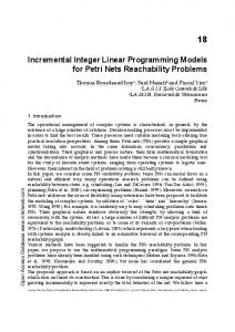
Experiment. through (5)) with the objective function term on X (c) dropped. The correspondence of Y*, Z*, UI, V*, W* and the shadow prices on equation (17) with their observed values and the prices of the products (c) can then be tested. Such a test accomplishes two purposes. First, given the real world quantities to be produced, the optimal levels of the production (Y') and input supply (Z') activities may be examined for consistency with those observed. Second, the imputed values of the resources (V and W*) may be examined for consistency with the observed imputed values. Thus, a test is made of the linear programming optimality conditions that a good is produced to the level at which its marginal cost equals its prevailing price. Further, the dual values associated with the quantity constraints (equati (17)) should be sufficiently close (by one or more of the criteria discussed later) to the market prices for the outputs. 4 These shadow prices, Figure 1, give a indication of the marginal cost of prodution at the observed quantities. Uder ct o etition this shado rie s price th e equal the market price. The input version of the test is essentially The model (equations (1) through (5)) is augmented by the constraint Z = Z with the eZ term dropped from the objective function. In this case, the experiment should generate dual variables which can be compared to prevailing market prices of inputs, Figure 2. Price Experiment. A third type of model validation experiment is the price experiment. This type of experiment is relevant in models where price is an endogenous vari-

Kutcher presents this procedure as a test of the economic assumption of perfect competition.

159

particular experiment represents an attempt to see whether the linear programming model can replicate agent or system behavior that has been observed. To some degree, this is

DUAL

——_—_______

the ultimate experiment in the series in that it shows whether a model can in fact replicate reality. However, to some extent, it ignores

-L

the reason most linear programming models

exist; that is, for comparative statics analysis. IMPLICIT VALUE

.MARGINAL

O

This implies a need for the next type of

experiment.

.PRODUCT INPUT (x.)

Change Experiment. Many linear programming models are not constructed to "find THE answer." Often the models are used to

Figure 2. Input Figure Input Quantity Experiment. Experiment.-

able (such as in the sector models reviewed in McCarl and Spreen) or in linear programming models with fixed demand requirements. This experiment involves fixing the objective function coefficients at existing real world levels for products and/or factors whose prices are endogenous to the model, then observing quantities (the dual of the named quantity experiment). The output price experiment is illustrated in Figure 3. The quantities produced (X*) may be compared to the observed levels (X). One may also examine how implicit fixed resource values are influenced in the experiment. PredictionExperiment. The prediction experiment is the most commonly used experiment for validating linear programming models by results.5 Some examples can be found in Barnett et al.; Brink and McCarl; and Hazell and Pomareda. With the prediction experiment, problem parameters are fixed at existing real world levels, the model is solved, and the solution values of the primal and dual variables are compared with the existing real world observed values. This

generate several solutions in studying the magnitude of adjustments. The testing of such a model involves an examination of how well the model predicts changes between alternative scenarios. In validation then one must have two real world situations and solve the model under the two situations to test its performance (as done by Hazell et al.). Here, a comparison is made between the change in the model solution variables (e.g., X; X2) and the change observed in the real world solution (X, - X2), Tracking Experiment. A model's proficiency for predicting a one time change in a real world system may not form an adequate framework for validation in analyses of system adjustments through time. For applications of this type (for example, Pieri et al.), the model can be solved using an appropriate series of parameter sets. The focus of the validation would then be on how well the model "tracks" over time with respect to the corresponding observed adjustments in the system. Again, comparisons are made between changes in the model solution and observed changes in the real world solution. Partial Tests

PRICE

The listed experiments were presented for a model as a whole. Obviously, in any par-

MARGINAL COST

ticular validation exercise, it may be desir-

able to perform experiments with some of the variables fixed at real world levels with other variables left unconstrained-an at-

OBSERVED PRICE

tempt to validate portions of the model. Often,

I—]|

\:~ __]—:~

~

this type of experiment will be necessary ;with large models because observations on all decision variables and/or shadow prices

xX OUTPU

Figure 3. Output Price Experiment. 5

(XI)

may not be readily available. Validation experiments may then be performed to require

This experiment is often undertaken prematurely before experiments such as those above are conducted.

160

sums of variables to equal observed real world levels, for example. A PROCEDURE FOR EMPLOYING A VALIDATION TEST There are several identifiable stages to the process of model validation. The purpose of this section is to briefly present steps for conducting one of the named experiments. Step 1. Specify the model(s) relying on relevant theory, experience, and/or precedence. Step 2. Enter the constraints and/or activities which hold the shadow prices and/or variable values at observed levels for the specific validation experiment at hand. Step 3. Solve the model(s). Step 4. Evaluate the solution(s). Is it infeasible, unbounded, or optimal? (a) If the model solution is infeasible, examine the results to find the cause of infeasibility. If this in not easily found, consider adding artificial variables to those rows which are suspected of creating the infeasibilities and solving the model again, Once the cause is found, go to Step 6. (b) If the model is unbounded, examine it to find the source. If this is difficult, consider first adding large upper bounds to the individual variables, then solving the augmented model and identifying which variables equal the large upper bounds. These will be the variables that are unbounded. Complete a hand budget for the unbounded variables, pricing each resource at the shadow prices, and attempt to discover the cause of the unbounded solution. Once the cause is found, go to Step 6. (c) If the solution is optimal, perform association tests to discover the degree of correspondence between the "real world" and the model solutions (except for the feasibility experiment). These tests should be conducted upon both the primal and dual variables. Step 5. If the model variables exhibit a sufficient degree of association, then: (a) do higher level validation experi ments and if desired, (b) determine whether the model is valid and proceed to use the model.

Step 6. If the model does not pass the validation tests, consider whether: (a) the data are consistent and correctly calculated, (b) the model structure provides an adequate representation of the real world system, and (c) the objective function is correctly

specified.

Procedures for recalculating model parameters will be problem specific. If, for example, all the variables have been fixed at "real world" levels and infeasibilities occur, unit input and/or output levels of production activities may be incorrect. If the data are considered accurate and model structure problems are suspected, one should consider whether: errors have been made in constructing the matrix; additional constraints are needed which have been omitted; constraints have been entered which are not really constraints; some variables have been omitted which are, in fact, important; or whether such factors as risk and/or willingness to adjust (i.e., flexibility constraints) should be entered into the model. If the model has been respecified either structurally or through its data, proceed back to Step 3 and repeat the validation test. If not, go to Step 7. Step 7. If the preceding steps do not lead to a valid model, one must decide whether to: (a) do demonstrations with an invalid model-assuming this is an approximately correct structure, (b) abandon the project, or (c) limit the scope of validation to a lesser set of variables (aiming at a less strict level of validation), subsequently qualifying model use. This may happen in many cases due to some considerations discussed subsequently.

EVALUATION CRITERIA FOR VALIDATION Discussion of association tests has been consciously omitted to this point. Such tests can be used to measure whether a set of model results approximate observed results. Quite a number of association tests have been 161

proposed and used-particularly within the simulation literature (Shannon; Anderson; Gass; or Johnson and Rausser, for example). These tests have been well presented elsewhere, so elaborate discussion is not needed. A brief summary of some alternative tests of association may be in order, however. Regression techniques have been used to measure the association of model solutions with observed values (for examples see Nugent; Rodriquez and Kunkel). Here, model results are regressed on observed valuesperfect association would be indicated by an intercept of zero and a slope of one. The Theil U test has been suggested by Leuthold for use in validation and an application to LP appears in Pieri'et al. This is a nonparametric "goodness-of-fit" test for evaluating the closeness of two vectors. Garret and Woodworth refer to the use of the G Index for validation-a procedure for comparing vectors of zeros and ones. In LP, such a procedure can be used for comparing sets of basic variables (an example can be found in Keith). Simple measures such as means, sums, mean absolute deviations, and correlation coefficients, have also been used in LP validation (Nugent; Kutcher; Hazell et al.). The authors have not found applications of Chi square, Kolmogrow-Smirnov, or various other "goodness-of-fit" tests to LP validation exercises. However, these techniques have been applied in simulation studies (see reviews in Anderson; Johnson and Rausser; Shannon; and Gass).

WHAT IF THE MODEL DOES NOT VALIDATE? From a practical standpoint, models do not always validate. A particular model will probably not validate initially. Since assumptions are made in the process of model building, failure to validate likely indicates that a subset of these assumptions is violated. Consequently, if a model fails validation tests, the relevant question is: What assumptions need to be corrected? Two different types of assumptions are present in linear programming models: algorithmic and modeling. The algorithmic assumptions are additivity, divisibility, certainty, and proportionality (Hillier and Lieberman, pp. 135-8). These assumptions, when severely violated, will cause validation tests to fail. The model designer then must consider whether these are the cause of fail162

ure. If so, the use of techniques such as separable, integer, nonlinear, or stochastic programming may be desirable to construct a new model. Modeling assumptions may also lead to an invalid linear programing solution. These assumptions embody the correctness of the objective function, variables, constraints, coefficients, and coefficient placements. Linear programming algorithms are quite useful in discovering violations of these assumptions. Linear programming solutions are also rather transparent. At an optimal solution, one may easily discover what resources were used, how they were used, and marginal resource values. Thus, when presented with an invalid solution, resource usage and resource valuation should be investigated. Models are most often invalid because of inconsistent data, bad coefficient calculation, bad coefficient placement, incomplete structure, or an incorrect objective function. Thus, common fixes for a model failing validation involve data respecification and/or structural corrections. When dealing with linear programming, there are several other aspects of the model which can lead to validation failures. An optimal solution to a linear program is characterized by the term basic, i.e., no more activities can be in the model than the number of constraints. For example, if a disaggregated regional model is constructed with a single constraint in each region, at most one activity will be produced in each region (if other constraints are not present in the model). This is ordinarily inconsistent with real world performance. Models then may be judged invalid because they overspecialize in production due to the nature of basic solutions. Several approaches may be taken when faced with this sort of inadequacy in a model solution. First, one may be satisfied with validating only aggregate results and not worrying about individual production resuits. Second, one may constrain the model to the observed solution and investigate whether this solution is an alternative optimal solution (which, as argued by Paris, may commonly occur). Third, one may recognize that a basic solution will not validate and enter constraints that limit the adjustment process of the activities within the model (flexibility constraints as above). Fourth, the model may be expanded by including risk considerations (Hazell et al.). Fifth, one may feel the model is structurally inadequate in that many of the factors that constrain

production may be inadequately portrayed in the model (see the arguments in McCarl). Such a situation leads to either one of two fixes: more constraints can be added or the activities within the model may be respecifled so they represent feasible solutions within omitted constraints. Models may also fail validation because of the objective function. Specification of the constraints identifies the set of possible solutions, while specification of the objective function determines which feasible solution will be optimal. Thus, the objective function must be carefully specified and reviewed (especially if a feasible real world solution can be investigated through the dual feasibility test). Finally, a correct objective function may for all practical purposes possess alternative optimal solutions, one of which is the desired solution (see Paris for discussion). Another phenomena may lead to difficulty with model validation, particularly within agricultural models. Activities, quite often, have to be performed in a fixed sequence through several time periods (for example, a rotation that includes a legume crop for soil enrichment). An annual model with activities of this type may well be invalid because the activities are not properly

sequenced after activities which must have occurred before (for example, acreages of the legume last year). Thus, unless the model has initial conditions identical to those in the "real world," it may be very difficult to validate. CONCLUDING COMMENTS Validation is an important concern within any modeling exercise. Awell validated model will have gone through both the validation by construct and validation by results phases with care exercised at all points. Unfortunately, although a model user may nominally b satisfied, true validation will never occur. However, through satisfactory completion of the experiments outlined, the level of satisfaction may be increased. Finally, one of the ultimate tests of validity deals with adoption of the model by the decisionmaker. Satisfactory validation via the procedure given is not sufficient for acceptance. A numerically valid model may solve the wrong problem and, thus will never be valid from the decisionmaker's viewpoint. Clearly, under these circumstances, validation in the broadest sense is only achievable by redefining the model which takes into account the true problem.

REFERENCES

Anderson, J. "Simulation: Methodology and Applications in Agricultural Economics." Rev. Marketing and Agr. Econ., 43(1974): 3-55.

Barnett, D., B. Blake, and B. McCarl. "Goal Programming via Multidimensional Scaling Applied to Senegalese Subsistence Farms." Amer. J. Agr. Econ., 64,4(1982): 720-7. Baumes, H. "A Partial Equilibrium Sector Model of U.S. Agriculture Open to Trade: A Domestic Agricultural and Agricultural Trade Policy Analysis." Ph.D thesis, Purdue University, 1978. Brink, L. and B. McCarl. "The Adequacy of a Crop Planning Model for Determining Income, Income Change, and Crop Mix." Can. J. Agr. Econ., 47(1979): 13-25. Day, R. and A. Cigno, editors. Modeling Economic Change: The Recursive Programming

Approach. Amsterdam: North-Holland Publishing Co., 1978. Fajardo, D., B. McCarl, and R. Thompson. "A Multicommodity Analysis of Trade Policy Effects: The Case of Nicaraguan Agriculture." Amer. J. Agr. Econ., 63,1(1981): 2331. Garret, H. and R. Woodworth. Statistics in Psychology and Education. New York: David

McKay Co., Inc., 1964. Gass, S. I. "Decision-Aiding Models: Validation, Assessment, and Related Issues for Policy Analysis." Operations Research, 31(1983): 603-31.

Hazell, P. and C. Pomareda. "Evaluating Price Stabilization Schemes with Mathematical Programming." Amer. J. Agr. Econ., 63,3(1981): 550-6. Hazell, P., R. Norton, M. Parthasarthy, and C. Pomareda. "The Importance of Risk in Agricultural Planning Models." ProgrammingStudiesfor Mexican AgriculturalPolicy,

R. Norton and L. Solis (eds.). New York: Johns Hopkins Press, 1981. Henderson, J. "The Utilization of Agricultural Land: A Theoretical and Empirical Inquiry." Rev. Econ. and Stat., 41(1959): 242-59. 163

Hillier, F. and G. Lieberman. Introduction to Operations Research. San Francisco: HoldenDay, Inc., 1967. House, P. and R. Ball, "Validation: A Modern Day Snipe Hunt: Conceptual Difficulties of Validating Models," in S.I. Gass (ed.), Validation and Assessment of Issues in Energy Models, Proceedings of a Workshop, National Bureau of Standards, Spec. Pub. 564, Washington, D.C.; 1980. Johnson, S. and G. Rausser, "Systems Analysis and Simulation: A Survey of Applications in Agricultural and Resource Economics." in L. Martin (gen. ed.), A Survey ofAgricultural Economics Literature, 2(1977): 157-301. Keith, Nancy, "Aggregation in Large-Scale Distribution Systems." Ph.D. thesis, Purdue University, 1978. Kutcher, G., "A Regional Agriculture Planning Model for Mexico's Pacific Northwest." in R. Norton and L. Solis (eds.), ProgrammingStudies for Mexican AgriculturalPolicy, Chapter 11, New York: Johns Hopkins Press, 1983. Leontief, W., "Quantitative Input-Output Relations in the Economic System of the United States." Rev. Econ. Studies, 18(1936): 105-25. Leuthold, Raymond M., "On the Use of Theil's Inequality Coefficients." Amer. J. Agr. Econ., 57,3(1975): 344-6. McCarl, B. "Cropping Activities in Agricultural Sector Models: A Methodological Proposal." Amer. J. Agr. Econ., 64,4(1982): 768-72. McCarl, B. and T. Spreen, "Price Endogenous Mathematical Programming as a Tool for Sector Analysis," Amer. J. Agr. Econ., 62,1(1980): 87-102. Miller, T. and R. Millar, "A Prototype Quadratic Programming Model of the U.S. Food and Fiber System." mimeo, CES-ERS-USDA and Department of Economics, Colorado State University, 1976. Nugent, J., "Linear Programming Models for National Planning: Demonstration of a Testing Procedure." Econometrica, 38(1970): 831-55. Paris, Q., "Multiple Optimal Solutions in Linear Programming Models." Amer. J. Agr. Econ., 63,4(1981): 724-7. Pieri, R., K. Meilke, and T. MacAuley, "North American-Japanese Pork Trade: An Application of Quadratic Programming." Can. J. Agr. Econ., 25(1977): 61-79. Rodriquez, G. and D. Kunkel, "Model Validation and the Philippine Programming Model." Agr. Econ. Res., 32(1980): 17-25. Sahi, R. and W. Craddock, "Estimation of Flexibility Coefficients for Recursive Programming Models-Alternative Approaches." Amer. J. Agr. Econ., 56,2(1974): 344-50. Shannon, R., "Simulation: A Survey with Research Suggestions." AIIE Transactions,7(1975): 289-301.

164