Jan 11, 2017 - HOOFS) using Regional Ocean Modeling System (ROMS) with the ... (ROMS), which is a state-of-the art ocean circulation model (Song et al., ...
TEHNICAL REPORT
Report No.: ESSO/INCOIS/ISG/TR/01(2017)
Validation of the simulations by the High-resolution Operational Ocean Forecast and reanalysis System (HOOFS) for the Bay of Bengal by Jithin A. K1, 2, Francis P. A1, Abhisek Chatterjee1, Suprit K1 and Vijayan Fernando3 1
Indian National Centre for Ocean Information Services (INCOIS) Ministry of Earth Sciences, Hyderabad-500090.
2Department
of Meteorology and Oceanography, Andhra University, Visakhapatnam, Andhra Pradesh-530003.
3National
Institute of Oceanography (NIO)
Dona Paula, Goa-403004.
11 January, 2017
DOCUMENT CONTROL SHEET Earth System Science Organization (ESSO) Ministry of Earth Sciences (MoES) Indian National Centre for Ocean Information Services (INCOIS) ESSO Document Number: ESSO/INCOIS/ISG/TR/01(2017) Title of the report: Validation of the simulations by the High-resolution Operational Ocean Forecast and reanalysis System (HOOFS) for the Bay of Bengal
Author(s) [Last name, First name]: Jithin A.K, Francis P. A, Abhisek Chatterjee, Suprit K and
Vijayan Fernando. Originating unit : Information and Services Group (ISG), INCOIS Type of Document : Technical Report (TR) Number of pages and figures : 56, 39 Number of references : 22 Keywords : Bay of Bengal, modeling, ROMS Security classification : Open Distribution : Open Date of publication : 11 January, 2017 Abstract (100 words) In this report, we present a detailed comparison and validation of the simulations from high-resolution (1/480) ocean circulation model for the Bay of Bengal (BBHOOFS) using Regional Ocean Modeling System (ROMS) with the available ocean observations and the simulations by the relatively lower resolution (1/120) basinscale general circulation model setup (IO-HOOFS), which is presently used to provide ocean forecasts for the Bay of Bengal. Comparison of vertical profiles of currents, temperature, Sea Level Anomaly (SLA) and Sea Surface Temperature (SST) for both model setups are carried for the period of 2013-2014. Comparison of the circulation features in the shelf and slope regions off the east coast of India simulated by the model with the ADCP observations shows that simulations by the BB-HOOFS are superior in terms of its ability to capture the features and variability in different space and time scales. In addition, simulations of currents by BB-HOOFS show high correlation and low RMSE values in the northern part of the shelf and slope off the east coast of India compared to south. Comparison of temperature simulations by the two model setups with observation shows that the simulations of BB-HOOFS is better, with high correlation and low RMSE values especially in the thermocline regions, compared to IO-HOOFS. However, comparison of SST and SLA simulated by BB-HOOFS with the satellite based observations is not showing any significant improvement compared to the simulations by IO-HOOFS.
Validation of the simulations by the High-resolution Operational Ocean Forecast and reanalysis System (HOOFS) for the Bay of Bengal Jithin A.K1, 2, Francis P. A1, Abhisek Chatterjee1, Suprit K1 and Vijayan Fernando3 1
Indian National Centre for Ocean Information Services (INCOIS) Ministry of Earth Sciences, Hyderabad-500090.
2Department
of Meteorology and Oceanography, Andhra University, Visakhapatnam, Andhra Pradesh-530003.
3National
Institute of Oceanography (NIO)
Dona Paula, Goa-403004.
INCOIS-Technical Report
January 2017
Abstract In this report, we present a detailed comparison and validation of the simulations from high-resolution (1/480) ocean circulation model for the Bay of Bengal (BB-HOOFS) using Regional Ocean Modeling System (ROMS) with the available ocean observations and the simulations by the relatively lower resolution (1/120) basin-scale general circulation model setup (IO-HOOFS), which is presently used to provide ocean forecasts for the Bay of Bengal. Comparison of vertical profiles of currents, temperature, Sea Level Anomaly (SLA) and Sea Surface Temperature (SST) for both model setups are carried for the period of 2013-2014. Comparison of the circulation features in the shelf and slope regions off the east coast of India simulated by the model with the ADCP observations shows that simulations by the BB-HOOFS are superior in terms of its ability to capture the features and variability in different space and time scales. In addition, simulations of currents by BB-HOOFS show high correlation and low RMSE values in the northern part of the shelf and slope off the east coast of India compared to south. Comparison of temperature simulations by the two model setups with observation shows that the simulations of BB-HOOFS is better, with high correlation and low RMSE values especially in the thermocline regions, compared to IO-HOOFS. However, comparison of SST and SLA simulated by BB-HOOFS with the satellite based observations is not showing any significant improvement compared to the simulations by IO-HOOFS.
1
Introduction Under the project “High-resolution Operational Ocean Forecast and reanalysis System (HOOFS)”, Indian National Centre for Ocean Information Services (INCOIS) has been carrying out focused research and development to configure a series of high-resolution ocean model setups to provide very high resolution operational forecast of various oceanographic parameters for the coastal waters around the country. Regional Ocean Modeling System (ROMS), which is a state-of-the art ocean circulation model (Song et al., 1994; Haidvogel et al., 2000; Shchepetkin, 2005) is used as the general circulation model for the HOOFS setups (Francis et al., 2013). Here we provide a detailed report of the performance of the model setup for the Bay of Bengal (BB-HOOFS) by comparing its simulations with the available ocean observations and the simulations by the basin-scale model setup, which is presently used to provide ocean forecasts for the Bay of Bengal. The Bay of Bengal (BoB) is a unique tropical bay located in the north-eastern part of the Indian Ocean bounded by land mass in the north. The region is well known for the surface low salinity water due to the large amount of freshwater influx from the adjacent continental rivers (Vinayachandran et al., 2015 and references therein). Presence of thick barrier layer is one of the factors affect the intensity of tropical cyclones in the Bay (Balaguru et al., 2014). Thermal inversions (Thadathil et al., 2002), meso-scale eddies (Chen et al., 2012) and the presence of locally and remotely forced waves (Cheng et al., 2013) complicates the variability in the Bay of Bengal and makes the numerical modeling of the Bay challenging. Hence, we do not expect a perfect simulation of the ocean conditions by any of the model configurations. However, here we try to quantify the improvements simulation of the general circulation features by the higher resolution model configuration so that it can be used for the operational predictions of ocean conditions with better accuracy.
2
2. Model domain and setup. In the present study, we compare the simulations by Regional Ocean Modeling System (ROMS, version 3.7), developed by Rutger’s University, New Jersey, USA, for the period of 2011 to 2015. ROMS is a free surface, terrain following general circulation model which solves a set of primitive equations in an orthogonal curvilinear coordinate system (Song et al., 1994; Haidvogel et al., 2000; Shchepetkin., 2005). Simulations from two different model setups, viz. one for the Bay of Bengal (BB-HOOFS) domain with very high spatial resolution (1/480) and the other for the entire Indian Ocean basin (IO-HOOFS, which is an improved version of the Indian Ocean model setup described in Francis et al 2013) with relatively lower resolution (1/120), are compared with the observations here. The bathymetry in the model domain for the IO-HOOFS setup is shown in Figure 1a. The domain of the Indian Ocean model based on ROMS extends from 30° E to 120° E in the east-west direction and from 30° S to 30° N in the north-south direction. The horizontal resolution of IO-HOOFS is 0.125° (approximately 13 km) and it has 40 sigma levels in the vertical. The vertical stretching parameters are chosen in such a way that the vertical resolution is highest in the upper part of the ocean. The lateral boundaries in the east and south are treated as open, where the tracer and momentum fields are nudged to 10-day mean fields derived from the INCOIS-GODAS analysis (Sivareddy et al., 2015). The western and northern boundaries are solid walls with noslip conditions. The model uses the KPP mixing scheme (Large et al., 1994) to parameterize the vertical mixing. Bi-harmonic diffusion and viscosity schemes are chosen for horizontal mixing and a bulk parameterization scheme (Fairall et al., 1994; Griffies and Hallberg, 2000) is chosen for the computation of air–sea fluxes of heat. Sea surface salinity is relaxed to the monthly climatological values derived from World Ocean Atlas (WOA) climatology (Antonov, et al., 2009; Locarnini, et al., 2009). 10 tidal
3
constituents derived from TPX07.2 are used to represent the realistic tides in the model. A detailed description of IO-HOOFS setup is provided in Francis et al (2013).
Fig. 1a: Model domain and bathymetry used in the IO-HOOFS setup.
Figure 1b shows the model domain and bathymetry (Modified etopo2, Sindhu et al., 2007, http://www.nio.org/index/option/com_subcategory/task/show/title/Sea-floor%20Data/ tid/2/sid/18/thid/113) used for the Bay of Bengal model setup (BB-HOOFS). The model domain covers entire Bay of Bengal and Andaman Sea, which extend from 77o E to 99o E and 4o N to 23o N. Malacca strait and Palk Strait are closed in the present model configuration. The spatial resolution of the model is 1/480 (approximately 2.23 km) in horizontal and 40 sigma levels in vertical. The south and west boundaries of the model setup is open and
4
nudged to the daily values of the basin-scale IO-HOOFS simulations. The model uses the KPP mixing scheme (Large et al., 1994) to parameterize the vertical mixing. Smagorinsky type viscosity and diffusion schemes (Muschinski, 1996) are chosen for horizontal mixing and a bulk parameterization scheme (Fairall et al., 1996) is chosen for the computation of air– sea fluxes of heat. Atmospheric fields from Global Forecast System (GFS) at a horizontal resolution of 1/4o, obtained from NCMRWF (http://www.ncmrwf.gov.in/t254-model /t254_des.pdf) are used for forcing both the BB-HOOFS and IO-HOOFS setups. In addition, model is incorporated with the tidal forcing from TPX07.2 model in the southern and western open boundaries. Sea surface salinity of this model setup is also relaxed to climatological values obtained from revised WOA for north Indian Ocean (Chatterjee et al., 2012).
Fig. 1b: Model domain and bathymetry used in the BB-HOOFS setup.
5
2. Data and methods Observations of current and temperature/salinity obtained from different observation platforms in the deep and coastal regions of BoB are used here to validate the model simulations from IO-HOOFS setup, which is presently used for the operational forecast at INCOIS, as well as the BB-HOOFS. Various parameters such as correlation, Root Mean Square Error (RMSE), standard deviation and bias are calculated on the model simulations to statistically quantify the performance both the model setups. All the analysis are carried by extracting model output into the observation grid and time. Data obtained from various observation platforms/moorings are used for the model validation during 2013-2014 are shown in Figure 2. Even though the model simulations are available from 2011 onwards, the period of model validation is restricted to 2013-2014 due to less coverage of simultaneous observation of current and temperature at various locations in the BoB during other years. In the coastal regions, current data are obtained from Acoustic Doppler current profilers (ADCP) deployed along the continental shelf and slopes off the east coast of India by National Institute of Oceanography (NIO), Goa, with the financial support from ESSOINCOIS. Vertical profiles of currents obtained from the ADCP moorings deployed along the continental shelf (6 ADCPs) and slope (5 ADCPs) off the east coast of India (Table 1) are used for the comparison of currents in the coastal regions. Shelf ADCPs were deployed about 150 - 200m depth and slope ADCPs were deployed about 1000m depth. The vertical resolution of shelf and slope ADCPs data are 4m and 8m, respectively. The data near to the surface and bottom levels were removed during the quality check due to the contamination and echoes. Daily average of current data between 24 - 150m from the shelf ADCPs and data between 40 - 500m from the slope ADCPs were used to compare with ROMS output. The period of data availability is given in Figure 3.
6
Fig. 2: Locations of coastal ADCPs and deep water moorings in the BoB used for the model validation.
7
Fig. 3: ADCP data availability on the shelf (green), slope (red) and deep regions (green) during 2013-2014 period in the BoB.
Deep ocean observations of current, temperature and salinity data are obtained from NIOT open ocean buoys and temperature/salinity data from RAMA (McPhaden et al., 2009), buoys (Fig. 2). Current, temperature and conductivity data obtained from Moored Buoy Network in Northern Indian Ocean (OMNI buoys) which is deployed and maintained by National institute of Ocean Technology (NIOT) are used for the comparison of model output in the deep water regions. These OMNI buoys are moored with ADCPs which measure current in the upper 105m. In addition, these moorings are attached with CTD sensors in the subsurface at various levels which measures temperature and conductivity up to 500m depth. All observations of temperature and currents are converted into daily averages for the model comparison. In addition, depth of 200 isotherm (d20) and Mixed Layer Depth (MLD) is
8
computed for all the mooring locations and statistics of the model performance are computed. Temperature data from RAMA buoys at 120 N and 150 N were also used for the comparison, whereas there is no/little data are available during 2013-2014 at 80 N, hence it excluded from the comparison. The period of data availability is given in Figure 3. Temperature/salinity data are obtained from coastal moored buoys deployed by National Institute of Ocean Technology (NIOT).
Fig. 4: Temperature data availability during 2013-2014 period in the BoB from coastal NIOT buoys (black), RAMA (pink) and OMNI buoys (green).
Temperature/salinity data from Argo profilers (https://www.nodc.noaa.gov/argo/ floats_data.htm) in the BoB during 2013-2014 are also used to validate the vertical structure 9
of temperature simulated by the model setups. About 7187 temperature and salinity profiles from Argo profiles are available in the BoB during 2013-2014 (Fig. 5). Data from Argo profilers in the BoB are categorized into western BoB (770 E - 900 E, 40 N - 160 N), eastern BoB (900 E - 990 E, 40 N - 160 N) and northern BoB (770 E – 990 E, 160 N - 230 N) and statistical analyses are carried out for each category separately. No. of profiles in each year and in different sections were shown in Figure 3. Statistics of temperature up to 2000m depth were calculated to show the model performance at various vertical levels. In addition, TRMM TMI (TRMM Micro-wave Imager) Sea Surface Temperature (SST, Kummerow et al., 1998; Wentz et al., 2000, http://www.remss.com/missions /tmi#data_access) data and daily Sea Level Anomaly data (SLA) from Copernicus Marine and Environment Monitoring Service (CMEMS, http://www.marine.copernicus.eu) are also used to validate the model simulations. The spatial resolution of TMI SST data is 0.250. The SST and SLA from the model output is regrided into observational grids and statistical parameters are computed. Since, surface salinity in the model setups are relaxed to climatological values, we excluded the comparison of salinity with the observation.
10
Fig. 5: Location of ARGO profiles in the BoB during 2013 (blue) and 2014 (red).
3. Results Currents, temperature and sea-level simulated by both the model setups are compared with the observations obtained from various platforms in the BoB during the period of 20132014. Comparison of time series data and its statistical parameters at all the locations in the BoB are given below.
3.1 Comparison of current in the coastal regions using ADCP data 3.1.1 Comparison of currents on the shelf Comparison of the time-depth sections of zonal (u) and meridional (v) currents simulated by the low resolution (IO-HOOFS) and the high-resolution (BB-HOOFS) model setups and the observations from the ADCPs installed on the shelf regions are shown along 11
with the vertical profiles of statistical parameters such as correlation, standard deviations, root mean square errors and biases in Figures 6-11. Locations of ADCPs on the shelf are shown in Figure 2. Current data about 25-150m depths from six ADCPs moorings are chosen for the comparison on the shelf. Cuddalore, the southernmost ADCP location, where the observed current flows towards the equator during January to April and its magnitude in this period is relatively strong compared to other periods. In addition, current is mostly unidirectional in the surface layers whereas slightly fluctuates below 75m during this period (January to April). During the period from May to December, currents on the shelf off Cuddalore flow poleward in the surface layers during May to December and an under currents flowing equatorward with large intraseasonal variability below 50m. Comparison of currents simulated from the models with the observation show that skill of capturing the temporal variation of currents (magnitude and direction) is significantly higher in the BBHOOFS setup compared to the IO-HOOFS on the shelf off cuddalore (Fig. 6). Further, vertical structure of current has improved and intraseasonal variabilities are more realistic in BB-HOOFS setup. Even though the correlation values of currents in the BB-HOOFS and IOHOOFS with observed currents are nearly same, RMSE is reduced significantly for meridional component and standard deviation (variance) becomes more closer to the observed values (Fig. 6). The observed variability of currents on the shelf off Kakinada is more or less similar to that on the shelf off Cuddalore with a less intraseasonal variability (Fig. 7). The intraseasonal variability of current are found to be diminishing towards the ADCP locations in the northern part of the shelf. In addition, observed currents start to flow in the northward direction much earlier in the northern locations compared southern location. For example, current start to flow towards north during the end of October on the shelf off Gopalpur whereas currents start to flow northward during January on the shelf off Cuddalore. The BB-HOOFS setup has captured these variation in the currents better compared to the IO-
12
HOOFS. Correlation of currents simulated by BB-HOOFS is higher than that of IO-HOOFS setup on the shelf off Kakinada. Further north, observed currents on the shelf off south of Visakhapatnam, Visakhapatnam and south of Gopalpur show dominant seasonal variability compared to intraseasonal variability (Fig. 8-10). Comparisons of time series of current simulations with ADCP observations at these locations show that BB-HOOFS is able captures similar pattern of variability. Further, statistical parameters computed for both the model setups show that BB-HOOFS simulated current are in better than IO-HOOFS simulations at these locations. There is a noticeable difference in BB-HOOFS performance from southern to northern part of the shelf. Current simulated by BB-HOOFS in the northern locations on the shelf shows a better comparison with the observation compared to south. For example, the correlation (RMSE) of BB-HOOFS with observation on the shelf off South of Gopalpur is larger (less) than those on the shelf off Cuddalore (Fig. 8 and 10). Similarly, BBHOOFS performance is better on the shelf off Gopalpur compared to southern ADCP locations. This clearly indicates that there is significant increase in model performance in the northern part of the shelf compared to south. This could be due to the dominance of higher order modes of variability, which are better simulated by high-resolution model compared to the lower resolution models in the higher latitudes compared to the lower latitudes. Observed currents on the shelf show variability in both seasonal and intraseasonal scales. One of the main difference in the performance of the two model setups is BB-HOOFS simulations is able to capture the intraseasonal variability better than IO-HOOFS. For example, BB-HOOFS simulate intraseasonal variability and observed under currents on the shelf of Cuddalore compared to IO-HOOFS (Fig. 6). Statistical parameters for currents for both model setups are not showing significant differences on the shelf off Cuddalore, however BB-HOOFS is capable of simulating intraseasonal variability better than IO-HOOFS. Similar improvements in current simulation by BB-HOOFS can found in all the ADCP location on the shelf. In the
13
case of seasonal variability, BB-HOOFS performance is substantially higher compared to IOHOOFS. For example, seasonal reversal of current on the shelf off Cuddalore, off Visakhapatnam, off Gopalpur is well simulated by BB-HOOFS setup. In short, current simulations from BB-HOOFS setup show good comparison with ADCP data compared to IO-HOOFS. Currents simulated by BB-HOOFS setup show significant improvements in the northern part of the shelf compared to south. Further, BBHOOFS is able to capture intraseasonal and seasonal variability better than IO-HOOFS.
14
Fig. 6: Comparison of u and v components of currents from ADCP (first panel), ROMS 1/480 (second panel) and ROMS 1/120 on the shelf off Cuddalore. Statistical parameters with depth are shown in the lowest panel.
Fig. 7: Comparison of u and v components of currents from ADCP (first panel), ROMS 1/480 (second panel) and ROMS 1/120 on the shelf off Kakinada. Statistical parameters with depth are shown in the lowest panel.
15
Fig. 8: Comparison of u and v components of currents from ADCP (first panel), ROMS 1/480 (second panel) and ROMS 1/120 on the shelf off south of Visakhapatnam. Statistical parameters with depth are shown in the lowest panel.
16
Fig. 9: Comparison of u and v components of currents from ADCP (first panel), ROMS 1/480 (second panel) and ROMS 1/120 on the shelf off Visakhapatnam. Statistical parameters with depth are shown in the lowest panel.
17
Fig. 10: Comparison of u and v components of currents from ADCP (first panel), ROMS 1/480 (second panel) and ROMS 1/120 on the shelf off south of Gopalpur. Statistical parameters with depth are shown in the lowest panel.
18
Fig. 11: Comparison of u and v components of currents from ADCP (first panel), ROMS 1/480 (second panel) and ROMS 1/120 on the shelf off Gopalpur. Statistical parameters with depth are shown in the lowest panel.
19
3.1.2 Comparison of currents on the slope Current data from ADCPs deployed at about 1000m depth off Cuddalore, Kakinada, Visakhapatnam, Gopalpur and Paradip are used to compare and validate model-simulated currents on the continental slope. Here, we restricted our analysis in 40-500 m depth. Timedepth sections of currents from the ADCPs and the model simulations are presented in Figure 12-16. In addition, the statistical parameters of the validation for both model setups are also shown. Seasonal and intraseasonal variability of currents on the slope is more less similar to that on the shelf locations. Both IO-HOOFS and BB-HOOFS setups are able to simulate the seasonal variability of currents at all the location on the slope, however IO-HOOFS is unable to capture the intraseasonal variability on the slope. For example, observed currents show significant intraseasonal variability on the slope off Cuddalore and Visakhapatnam, while IOHOOFS is not able to capture these variability in detail (Fig. 12 and 14). Observed currents shows that intraseasonal variability of currents on the slope off Paradip is lesser compared to other locations and current shows strong seasonal variability. Current simulated by BBHOOFS is able to capture the seasonal variability better than IO-HOOFS on the slope off Paradip (Fig. 16). ADCP observations off Cuddalore, Visakhapatnam and Gopalpur clearly show an undercurrent flowing poleward below 75 m depth whereas surface current flows towards equator on the slope. The presence of under current is also observed on shelf locations, but it is more visible on the slope. Current simulations from BB-HOOFS setup show the presence of undercurrent on the shelf and able to capture it’s the variability better than IO-HOOFS setup (Fig. 12 and 14). In addition, IO-HOOFS simulated under currents are deeper than observed currents and with less intraseasonal variability and often failed to simulate the under current (Fig. 13 and 15).
20
In general, comparison of model-simulated currents with observations shows that BBHOOFS simulated currents have a high correlation and low RMSE compared to IO-HOOFS setup except on the slope off Kakinada. Further, comparison of statistical parameters for current simulations from BB-HOOFS at different locations show a spatial variability in the model performance. In the northern part of the slope (off Visakhapatnam and Gopalpur), BBHOOFS simulated currents show higher correlation, low RMSE and better agreement in standard deviation compared to locations in the south. This suggests that current simulations from BB-HOOFS setup is better in the ADCP locations in the north compared to south.
Fig. 12: Comparison of u and v components of currents from ADCP (first panel), ROMS 1/48
21
(second panel) and ROMS 1/12 on the slope off Cuddalore. Statistical parameters with depth are shown in the lowest panel.
Fig. 13: Comparison of u and v components of currents from ADCP (first panel), ROMS 1/480 (second panel) and ROMS 1/120 on the slope off Kakinada. Statistical parameters with depth are shown in the lowest panel.
22
Fig. 14: Comparison of u and v components of currents from ADCP (first panel), ROMS 1/480 (second panel) and ROMS 1/120 on the slope off Visakhapatnam. Statistical parameters with depth are shown in the lowest panel.
23
Fig. 15: Comparison of u and v components of currents from ADCP (first panel), ROMS 1/480 (second panel) and ROMS 1/120 on the slope off Gopalpur. Statistical parameters with depth are shown in the lowest panel.
24
Fig. 16: Comparison of u and v components of currents from ADCP (first panel), ROMS 1/480 (second panel) and ROMS 1/120 on the slope off Paradip. Statistical parameters with depth are shown in the lowest panel.
25
3.2 Comparison of currents in the deep regions ADCP data from NIOT OMNI buoys are used to validate the model simulations in the deep BoB. Data from 7 ADCPs are available in the BoB and one from the Andaman sea which all recorded current data in the upper 105m depth. The location of OMNI buys are given in Figure 2 and comparison at BD013a, BD14a and BD14b moorings only are presented here as there are significant gaps in the data from other locations. Time-depth sections of both eastward and northward components of currents with observations and vertical structure of statistical parameters of validations are shown in Figures 17-22. Comparison show that BB-HOOFS simulated currents are good agreement with observation compared to IO-HOOFS. Correlation of BB-HOOFS simulated currents with observation is higher than that of IO-HOOFS setup at all the locations except at BD10. The correlation of both models in the upper layers (0-20 m) is nearly same but below 20m, correlation of BBHOOFS setup is found to be higher than IO-HOOFS setup. This indicates that BB-HOOFS setup shows a significant improvements in the simulation of currents in the deeper levels. In addition to the observations from BoB, data from one ADCP mooring is available for Andaman Sea (BD12 mooring). Analysis shows that there is a good improvement in the simulations of BB-HOOFS setup in this region also. The there is no significant spatial variation in the BB-HOOFS model performance in the deep regions.
26
Fig. 17: Comparison of u and v components of currents from ADCP (first panel), ROMS 1/480 (second panel) and ROMS 1/120 at BD08. Statistical parameters with depth are shown in the lowest panel.
27
Fig. 18: Comparison of u and v components of currents from ADCP (first panel), ROMS 1/480 (second panel) and ROMS 1/120 at BD09. Statistical parameters with depth are shown in the lowest panel.
28
Fig. 19: Comparison of u and v components of currents from ADCP (first panel), ROMS 1/480 (second panel) and ROMS 1/120 at BD10. Statistical parameters with depth are shown in the lowest panel.
29
Fig. 20: Comparison of u and v components of currents from ADCP (first panel), ROMS 1/480 (second panel) and ROMS 1/120 at BD11. Statistical parameters with depth are shown in the lowest panel.
30
Fig. 21: Comparison of u and v components of currents from ADCP (first panel), ROMS 1/480 (second panel) and ROMS 1/120 at BD12. Statistical parameters with depth are shown in the lowest panel.
31
Fig. 22: Comparison of u and v components of currents from ADCP (first panel), ROMS 1/480 (second panel) and ROMS 1/120 at BD13b. Statistical parameters with depth are shown in the lowest panel.
32
3.3 Comparison of Temperature 3.3.1 Comparison with NIOT Buoys and RAMA buoys data Temperature simulated by both the model setups are compared with the observation obtained from NIOT OMNI buoys and from the RAMA buoys in the BoB. Locations of OMNI buoys and RAMA buoys are shown in Figure 2. Temperature data from surface to 500m depth are used for the comparisons. Time-depth sections of observed temperature and model simulations in the upper 300 m along with the statistical parameters up to 500m are shown in Figures 23-32. A comparison of the performance of both the model configurations in simulating the observed mixed layer depth also is shown in Figure 33 as a Taylor diagram. Comparison shows that correlation of BB-HOOFS is slightly higher than IO-HOOFS in the upper 25 m whereas a significant increases in correlation temperature simulated by BBHOOFS setup is observed below 25 m, particularly in the thermocline regions. This improvements is almost consistent at all NIOT buoy and RAMA buoy locations. For example, BB-HOOFS simulated temperature at BD10 shows no improvements in upper 20m but below 20 m, model shows a significant increase in correlation with observation (Fig. 25). Further, model comparison with temperature data obtained from RAMA buoys also show higher correlation in the in the thermocline region compared to surface layers. Relatively less improvement in the quality of simulations by BB-HOOFS compared to the IO-HOOFS near the sea surface could be due to the fact that the air-sea fluxes, which significantly influence the surface processes for both the model configurations are derived from the same atmospheric forcing fields. Observed temperature shows significant variability in the intraseasonal time scale in the BoB and BB-HOOFS setup capture this intraseasonal variability better compared to IOHOOFS. For example, the vertical temperature profiles at BD08 and BD09 show considerable intraseasonal variability during the July – December 2014 (Fig. 23 and 24).
33
Temperature simulations from BB-HOOFS setup show similar variability but IO-HOOFS setup is failed to capture this variability at these locations. Another important feature of temperature profile of Bay of Bengal is the thermal inversions, particularly in the late winter and early spring. Observations from most of the mooring locations clearly show these inversions. Both the model setups are able to capture this features. However, inversions in the IO-HOOFS setup simulations are stronger than the observed temperature inversions and often simulate unrealistic inversions. For example, temperature inversions during January-March 2014 at BD10 (Fig. 25). The temperature inversions simulated by BB-HOOFS are more realistic and in good agreement with observations. Further, observations show that surface layers are warmer during summer and cooler during winter in the BoB, Both model setups are able to capture this seasonal warming and cooling of surface layers and BB-HOOFS simulations are in good agreement with observation. For example. IO-HOOFS simulations are not showing cooling of surface layers during November 2013 - February 2014 at BD12 (Fig. 27).
34
Fig. 23: Comparison of temperature from OMNI buoy BD08 (first panel), ROMS 1/480 (second panel) and ROMS 1/120. Statistical parameters with depth are shown in the lowest panel.
35
Fig. 24: Comparison of temperature from OMNI buoy BD09 (first panel) with ROMS 1/48 (second panel) and ROMS 1/12. Statistical parameters with depth are shown in the lowest panel.
36
Fig. 25: Comparison of temperature from OMNI buoy BD10 (first panel) with ROMS 1/48 (second panel) and ROMS 1/120. Statistical parameters with depth are shown in the lowest panel.
37
Fig. 26: Comparison of temperature from OMNI buoy BD11b (first panel) with ROMS 1/480 (second panel) and ROMS 1/120. Statistical parameters with depth are shown in the lowest panel.
38
Fig. 27: Comparison of temperature from OMNI buoy BD12 (first panel) with ROMS 1/480 (second panel) and ROMS 1/120. Statistical parameters with depth are shown in the lowest panel.
39
Fig. 28: Comparison of temperature from OMNI buoy BD13a (first panel) with ROMS 1/480 (second panel) and ROMS 1/120. Statistics are shown in the right panels.
40
Fig. 29: Comparison of temperature from OMNI buoy BD13b (first panel) with ROMS 1/480 (second panel) and ROMS 1/120. Statistical parameters with depth are shown in the lowest panel.
41
Fig. 30: Comparison of temperature from OMNI buoy BD14a (first panel) with ROMS 1/480 (second panel) and ROMS 1/120. Statistical parameters with depth are shown in the lowest panel.
42
Fig. 31: Comparison of temperature from RAMA buoy at 120 N, 900 E (first panel) with ROMS 1/480 (second panel) and ROMS 1/120.
43
Fig. 32: Comparison of temperature from RAMA buoy at 150 N, 900 E (first panel) with ROMS 1/480 (second panel) and ROMS 1/120.
44
Fig. 33: Taylor diagram for mixed layer depth comparison of ROMS 1/480 (second panel) and ROMS 1/120 simulations a different location.
Temperature simulations from IO-HOOFS and BB-HOOFS model setups are also compared with temperature observations obtained from NIOT coastal moored buoys. Comparison of time depth sections of temperature at CB01 and CB05 with model-simulated temperature are shown in Figure 34. This shows that BB-HOOFS simulated temperature capture most of the observed seasonal and intraseasonal variability compared to IO-HOOS, particularly at CB05.
45
Fig. 34: Comparison of temperature from coastal moored buoys with ROMS 1/480 and ROMS 1/120 in the entire BoB.
3.3.3 Comparison with ARGO data Vertical profiles of the RMSE, Correlation Coefficients, Standard Deviations and the Biases of the co-located temperature profiles simulated by two configurations of the model (viz. IO-HOOS and BB-HOOFS) with respect to the Argo profiles in the BoB during 20132014 period are shown in Figures 35-37. The comparison is carried out separately for entire BoB and for each regional sections, categorized as western BoB, Northern BoB and Eastern
46
BoB (see Fig. 5). The details of each sections are given in section 2 and results for the comparison in the Eastern BoB box are excluded due to the non-availability of sufficient Argo profiles. The statistical parameters for the model comparison of temperature data entire BoB shows that correlation (RMSE) of BB-HOOFS are greater (less) than that of IO-HOOFS (Fig. 32). As in the case of the comparisons with the moored buoy data in the surface layers, BB-HOOFS simulations are not showing any significant improvements in correlation or RMSE compared to IO-HOOFS. However, in the subsurface, especially in the thermocline region, the BB-HOOFS shows significant improvements. For example, the correlation values for BB-HOOFS in the upper 50 m is more or less similar to IO-HOOFS, but those in the depths about 50-800 m is high compared to IO-HOOFS. Similar results are also obtained from the comparison of temperature using NIOT and RAMA buoys observation. Further, regional wise comparison of temperature also show higher correlation and low RMSE values in the thermocline regions for the BB-HOOS simulations and the BB-HOOFS model performance is relatively better in the northern BoB compared to eastern and western BoB (Fig. 36 and 37).
47
Fig. 35: Comparison of temperature from ARGO with ROMS 1/480 and ROMS 1/120 in the entire BoB.
48
Fig. 36: Comparison of temperature with ROMS 1/480 and ROMS 1/120 in the Western BoB.
Fig. 37: Comparison of temperature with ROMS 1/480 and ROMS 1/120 in the Northern BoB
49
3.6 Comparison of SST and SLA The SST data from TMI sensors in TRMM and gridded SLA data from satellite altimetry are used to compare and validate the simulations from IO-HOOFS and BB-HOOFS setups. Spatial pattern of correlation of SST and SLA for both model simulations are nearly same and there is no noticeable improvements in BB-HOOFS simulations compared to IOHOOFS (Figs. 38-39). However, there is significant decrease in the RMSE values and bias in the SST and SLA in the simulations of BB-HOOFS compared to that of IO-HOOFS particularly in the northern and eastern part of BoB.
50
Fig. 38: Comparison of SST from ROMS 1/480 and ROMS 1/120 simulations with TMMR TMI SST data. Statistical parameters such as correlation (first panel), RMSE (second panel), BIAS (third panel) and standard deviation (bottom panel) are shown.
51
Fig. 39: Comparison of SLA from ROMS 1/480 and ROMS 1/120 simulations with satellite altimetry data. Statistical parameters such as correlation (first panel), RMSE (second panel), BIAS (third panel) and standard deviation (bottom panel) are shown.
Summary and conclusions In this report, we present the results of the comparison of the performance of two different ROMS model setups, viz. one for the Bay of Bengal (BB-HOOFS) domain with very high spatial resolution (1/480) and the other for the entire Indian Ocean basin (IOHOOFS) with relatively lower resolution (1/120) in simulating the general circulation features in the Bay of Bengal. Comparison of vertical profiles of currents, vertical profiles of temperature, SLA and SST for both model setups are carried for the period of 2013-2014. Comparison of the circulation features in the shelf and slope regions simulated by the model with the ADCP observations shows that simulations by the BB-HOOFS are superior in terms of its ability to capture the intraseasonal variability, under currents etc. It is observed that the simulations of currents by BB-HOOFS show high correlation and low RMSE values in the northern part of the shelf and slope compared to south. Similarly, comparison of temperature simulations by the two model setups with observation from NIOT, RAMA buoys and Argo profiling floats shows that the simulations of BB-HOOFS is better, with high correlation and low RMSE values especially in the thermocline regions, compared to IO-
52
HOOFS. Seasonal and intraseasonal variability in the vertical temperature structure is also better simulated by the BB-HOOFS and temperature inversions is more realistic compared to IO-HOOFS simulations. Comparison of SST and SLA simulated by BB-HOOFS with the satellite based observations is not showing any significant improvement in the correlation coefficients compared to the simulations by IO-HOOFS. However, it is found that the RMSE and bias in SLA and SST simulations by BB-HOOFS is relatively less compared to the simulations by IO-HOOFS.
Acknowledgements This work was done as part of 'High-resolution Operational Ocean Forecast and reanalysis (HOOFS)' project of ESSO-INCOIS. RAMA data used in this study is taken from http://www.pmel.noaa.gov/tao/drupal/disdel/. We thank the developers of the ROMS model. The National Centre for Medium Range Weather Forecasting (NCMRWF), New Delhi is acknowledged for making the atmospheric analysis and forecast products available for the ROMS simulations. The altimeter products were produced by SSALTO/DUCAS and distributed by Copernicus Marine and Environment Monitoring Service (CMEMS, http://www.marine.copernicus.eu).
Argo
profile
data
is
downloaded
from
https://www.nodc.noaa.gov/argo/floats_data.htm. The TRMM TMI data used for the comparisons are produced by remote sensing systems and sponsored by the NASA Earth Science MEaSUREs DISCOVER project (http://www.remss.com/missions /tmi#data_access). OMNI buoys are deployed and maintained by the Ocean Observations Systems (OOS) group of ESSO-NIOT. Authors sincerely thank all those who provided data for this analysis.
53
References Antonov, J. I. et al., 2009 World Ocean Atlas 2009. Volume 2: Salinity. (ed. Levitus, S.), NOAA Atlas NESDIS 69, US Government Printing Office, Washington, DC, 2010, p. 184.20. Balaguru, K., Taraphdar, S., Leung, L.R., Foltz, G.R., 2014. Increase in the intensity of postmonsoon Bay of Bengal tropical cyclones, Geophysical Research Letters. 41 (10), 3594-3601 Chatterjee, A., Shankar, D., Shenoi, S.S.C., Reddy, G.V., Michael, G.S., Ravichandran, M., Gopalkrishna, V.V., Rao, E.P.R., Bhaskar, T.V.S.U., Sanjeevan, V.N., 2012. A new atlas of temperature and salinity for the North Indian Ocean. Journal of Earth System Science, 121, No.3, pp. 559-593; doi: 10.1007/s12040-012-0191-9. Chen G, D. Wang, Y. Hou., 2012. The features and interannual variability mechanism
of
mesoscale eddies in the Bay of Bengal, Continental Shelf Research, http://dx.doi. org/10.1016 /j.csr.2012.07.011. Cheng, X., S.-P. Xie, McCreary, J. P., Qi, Y., Du, Y., 2013. Intraseasonal variability of sea surface height in the Bay of Bengal. Journal of Geophysical Research: Oceans., 118 , 816–830, doi:10.1002/jgrc.20075. Fairall, C. W., Bradley, E. F., Rogers, D. P., Edson, J. B. and Young, G. S., 1996. Bulk parameterization of air–sea fluxes for TOGA COARE. Journal of Geophysical Research., 101, 3747– 3764. Francis, P.A., Vinayachandran, P. N., Shenoi, S. S. C., 2013. The Indian Ocean Forecast System. Current Science., Vol. 104, No. 10, 25,1354-1368p. Griffies, S. M., Hallberg, R. W., 2000. Biharmonic friction with a Smagorinsky-like Viscosity for use in large-scale eddy-permitting Ocean models. Mon. Weather Rev., 54
2000, 128, 2935–2946; doi: http://dx.doi.org/10.1175/1520- 0493(2000)1282.0.CO;2. Haidvogel, D. B., Arango, H. G., Hedstrom, K., Beckmann, A., Malanotte-Rizzoli, P. and Shchepetkin, A. F., 2000. Model evaluation experiments in the North Atlantic Basin: simulations in nonlinear terrain-following coordinates. Dyn. Atmos. Oceans. 32, 239–281. Kummerow, C., Barnes, W., Kozu, T., Shiue, J. and Simpson, J., 1998. The tropical rainfall measuring mission (TRMM) sensor package. Journal of Atmosphere and Ocean Technology., 1998, 15, 809–817. 26. Large, W. G., McWilliams, J. C. and Doney, S. C., 1994. Oceanic vertical mixing: a review and a model with a nonlocal boundary layer parameterization. Reviews of Geophysics., 32, 363–403. Locarnini, R. A. et al., 2009. World Ocean Atlas 2009, Volume 1: Temperature (ed. Levitus, S.), NOAA Atlas NESDIS 68, US Government Printing Office, Washington, DC, 2010, p. 184. McPhaden, M. J. et al., 2009. Supplement to RAMA: The Research Moored Array for African-Asian–Australian Monsoon Analysis and Prediction. Bulletin of American Meteorological
Society.,
90,
ES5–ES8;
doi:
http://dx.doi.org/10.1175/2008
BAM S2608.2. Muschinski, A., 1996. A similarity theory of locally homogeneous and isotropic turbulence generated by a Smagorinsky-type LES. Journal of Fluid Mechanics., 325, 239–260. Sivareddy, S., Ravichandran, M., Girishkumar, M.S. and Prasad, K.V.S.R., 2015. Assessing the impact of various wind forcing on INCOIS-GODAS simulated ocean currents in the equatorial Indian Ocean. Ocean Dynamics, 65(9-10), pp.1235-1247.
55
Shchepetkin, A. F., McWilliams, J. C., 2005. The regional ocean modeling system (ROMS): A split-explicit, free-surface, topography-following-coordinate oceanic model. Ocean Modelling., 2005,9/4, 347–404; doi: 10.1016/j.ocemod.2004.08.002. Sindhu, B., Suresh, I., Unnikrishnan, A.S., Bhatkar, N.V., Neetu, S., Michael, G.S., 2007. Improved bathymetric data sets for the shallow water regions in the Indian Ocean. Journal of Earth System Science 116, 261–274. Simpson, J., Kummerow, C., Tao, W.-K., Adler, R. F., 1996. On the Tropical Rainfall Measuring Mission (TRMM). Meteor. Atmos. Phys., 60, 19–36. Song, Y. and Haidvogel, D. B., A semi-implicit ocean circulation model using a generalized topography-following coordinate system. Journal of Computational Physics., 1994, 115, 228–244. Thadathil, P., Gopalakrishna, V. V., Muraleedharan, P. M., Reddy, G. V., Araligidad, N., Shenoy, S.S.C., 2002, Surface layer temperature inversion in the Bay of Bengal, Deep Sea Research., Part I , 49 , 1801–1818. Vinayachandran, P.N., Shankar, D., Vernekar, Siddharth., Sandeep, K.K.,
Amol, P.,
Neema, C.P., Chatterjee, A., 2013. A summer monsoon pump to keep the Bay of Bengal salty. Geophysical Research Letters, 40 (9). pp. 1777-1782. Wentz, F. J., Gentemann, C. L., Smith, D. K., Chelton, D. B., 2000. Satellite measurements of sea-surface temperature through clouds. Science, 2000, 288, 847–850.
56