Hindawi Complexity Volume 2018, Article ID 2825483, 13 pages https://doi.org/10.1155/2018/2825483
Research Article Valuation on an Outside-Reset Option with Multiple Resettable Levels and Dates Guangming Xue,1 Bin Qin,1 and Guohe Deng 1
2
School of Information and Statistics, Guangxi University of Finance and Economics, Nanning 530003, China School of Mathematics and Statistics, Guangxi Normal University, Guilin 541004, China
2
Correspondence should be addressed to Guohe Deng;
[email protected] Received 14 October 2017; Accepted 22 February 2018; Published 8 April 2018 Academic Editor: Michele Scarpiniti Copyright © 2018 Guangming Xue et al. This is an open access article distributed under the Creative Commons Attribution License, which permits unrestricted use, distribution, and reproduction in any medium, provided the original work is properly cited. This paper studies an outside-reset option with multiple strike resets and reset dates, in which the strike price is adjusted by an external process associated with the underlying risky asset. We obtain analytical pricing formula for this option and the hedging parameters Delta and Gamma. Furthermore, some numerical examples are provided to analyze some characteristics of the outsidereset option and to examine the impacts of the external parameters on option prices and Greeks. These results show that the external process can significantly affect option prices and Greeks.
1. Introduction Reset options, whose strike price will be adjusted to a new strike price only on each of a set of prespecified dates if the stock price is below one of the reset levels, have greatly evolved in the past two decades. This reset clause embedded in derivative products can protect the investors amidst stock price declines. This makes a reset option useful in portfolio insurance (see, e.g., Boyle et al. [1]). There are only a few articles studying the reset options in the academic literature. Gray and Whaley [2] were the first ones to examine the value of S&P 500 index bear market warrants with a periodic reset feature. In their other paper (see Gray and Whaley [3]), they provided an explicit formula for the reset option with a periodic reset date. Hsueh and Guo [4], on the other hand, analyzed the multiple reset feature that is included in most covered warrants traded in Taiwan. More recently, Cheng and Zhang [5] discussed the pricing and hedging of reset options and propose a closedform pricing formula for this increasingly popular derivative instrument. Li et al. [6] derived a generalization of price formula for the reset call options with predetermined rates when the spot interest rate and volatility of stock are all time-dependent and deterministic. Liu et al. [7] evaluated the pricing of reset options when the underlying assets are
autocorrelated. Franc¸ois-Heude and Yousfi [8] proposed a general valuation of reset option studied in Gray and Whaley [2] in which all options are replaced by ATM (At-The-Money) ones. Subsequent contributions include analytic extensions to multiple reset rights with shouting moment of Dai et al. [9, 10], Dai and Kwok [11], Yang et al. [12], and Goard [13], step (or snapshot)-reset design of Hsueh and Liu [14], and Yu and Shaw [15], average trigger reset clauses of Kao and Lyuu [16], Liao and Wang [17], Kim et al. [18], Chang et al. [19], Dai et al. [20], and Costabile et al. [21, 22], window reset option with continuous reset constraints of Hsiao [23], and reset rights embedded in the Quanto options of Chen and Jiang [24]. In general, the reset call option with 𝑚 predetermined reset dates 0 < 𝑡1 < 𝑡2 < ⋅ ⋅ ⋅ < 𝑡𝑚 < 𝑇 has a payoff at a fixed maturity 𝑇 of 𝑉 (𝑇) = max {𝑆𝑇 − min [𝐾0 , 𝑆𝑡1 , 𝑆𝑡2 , . . . , 𝑆𝑡𝑚 ] , 0} ,
(1)
where 𝑆𝑡 denotes the underlying asset price at time 𝑡 and 𝐾0 denotes the initial strike price of option. In a real application, the terminal payoff of reset call option is usually set as +
𝑉 (𝑇) = max {𝑆𝑇 − 𝐾∗ , 0} = (𝑆𝑇 − 𝐾∗ ) ,
(2)
2
Complexity
where 𝐾∗ is defined by 𝐾0 , { { { { 𝐾∗ = {𝐾𝑗 , { { { {𝐾𝑑 ,
if min [𝑆𝑡1 , 𝑆𝑡2 , . . . , 𝑆𝑡𝑚 ] ≥ 𝐷1 , if 𝐷𝑗 > min [𝑆𝑡1 , 𝑆𝑡2 , . . . , 𝑆𝑡𝑚 ] ≥ 𝐷𝑗+1 , 𝑗 = 1, 2, . . . , 𝑑 − 1, if 𝐷𝑑 > min [𝑆𝑡1 , 𝑆𝑡2 , . . . , 𝑆𝑡𝑚 ] ,
where 𝐾𝑗 , 𝑗 = 1, 2, . . . , 𝑑, denote the strike price resets such that 𝐾0 > 𝐾1 > 𝐾2 > ⋅ ⋅ ⋅ > 𝐾𝑑 > 0 and 𝐷𝑗 , 𝑗 = 1, 2, . . . , 𝑑, are the reset levels. In particular, there is only one reset price when 𝑑 = 1. For valuation on the general-reset options, Liao and Wang [25] provided an explicit pricing formula of this option and analyzed the phenomena of Delta jump and Gamma jump across reset dates. In fact, there is essentially no explicit pricing formula for the discrete reset options, except when they resort to multivariate cumulative normal distribution function. A common disadvantage of the reset option whose payoff is defined in (1), however, is that the reset trigger depends on the underlying asset price alone. This exposes the holder and the writer of the reset option to the risk that the counterparty may manipulate the underlying asset price such that the payoff of the reset option being benefits according to the 𝐾0 , { { { { 𝐾∗ = {𝐾𝑗 , { { { {𝐾𝑑 ,
(3)
counterparty favorable way. In other words, the strike price reset event is triggered by a price fluctuation intentionally caused by the counterparty. In order to prevent such price manipulation, reset options have been innovated where the trigger event does not depend on the underlying asset price but on an external variable 𝑌𝑡 . For example, the underlying asset may be a foreign stock and the external variable may be an average of the underlying asset, the exchange rate or another asset correlating with the underlying asset. We will study different reset conditions imposed on a distinct but correlated underlying asset process. Such reset conditions are often called outside resets (see Heynen and Kat [26] and Kwok et al. [27]), and they are rather less studied than the regular type defined in (1). In this paper we propose an outside-reset option where the strike price 𝐾∗ is replaced by
if min [𝑌𝑡1 , 𝑌𝑡2 , . . . , 𝑌𝑡𝑚 ] ≥ 𝐷1 , if 𝐷𝑗 > min [𝑌𝑡1 , 𝑌𝑡2 , . . . , 𝑌𝑡𝑚 ] ≥ 𝐷𝑗+1 , 𝑗 = 1, 2, . . . , 𝑑 − 1,
(4)
if 𝐷𝑑 > min [𝑌𝑡1 , 𝑌𝑡2 , . . . , 𝑌𝑡𝑚 ] .
This novel design of using the external variable 𝑌𝑡 as a reset trigger replacing the underlying asset 𝑆𝑡 , as in the general-reset option specified in (2) and (3), offers three important advantages to both issuers and investors. First, the outside-reset option reduces the price manipulation around the reset level. Second, the outside-reset specification rules out jumps in Delta and thus makes the reset option more amenable to dynamic hedging. Finally, the outside-reset option provides a strike price correlated with an external variable fluctuation. The payoff that comes with these mentioned advantages above is complexity. The outside-reset option contains a simultaneous generalization of the reset option discussed by Liao and Wang [25] and a multivariate-based option of which both have a number of useful applications. For example, the arithmetic average reset options listed on the Taiwan Stock Exchange used an average of the stock prices as a trigger variable for reset. A barrier option on one or multiple assets with single external barrier also used other assets as resettable barrier variables for determining whether the options knock in or out. For valuation on these options, one can look to Cheng and Zhang [5], Liao and Wang [17], Kim et al. [18], Costabile et al. [22], Zhang [28], and so forth.
This paper is to discuss the pricing problem of the outside-reset option, defined by (2) and (4), and has two contributions. The first is to derive the analytical pricing formula for the outside-reset option under the proposed model. Furthermore, we provide the analytical pricing formula for the outside-reset option with 𝑑 strike resets and continuous reset dates, which is the limiting case of that with a set of discrete reset dates, and the hedging parameters Delta and Gamma. The second is to analyze the impacts of the external process on the option price and the values of Delta and Gamma and the phenomena of Delta and Gamma jumps across reset dates using numerical experiments. The paper is organized as follows: in Section 2, a closedform pricing formula is derived first for the outside-reset option under the assumption that the underlying asset price process and the external process follow two correlation geometric Brownian motions. In Section 3, we discuss some properties of the outside-reset option and present our numerical results. Finally, in Section 4, we give conclusion remarks and directions of future research.
Complexity
3
2. The Proposed Model and Pricing Outside-Reset Option
From (8), we know that the key of solution is to compute the following expression:
Following Heynen and Kat [26], we consider the two stochastic differential equations for the underlying risky asset price 𝑆𝑡 and the external process 𝑌𝑡 (as a reset trigger) under a riskneutral measure 𝑄: 𝑑𝑌𝑡 = 𝑟𝑑𝑡 + 𝜎1 𝑑𝑊𝑡1 , 𝑌𝑡 𝑑𝑆𝑡 = 𝑟𝑑𝑡 + 𝜌𝜎2 𝑑𝑊𝑡1 + √1 − 𝜌2 𝜎2 𝑑𝑊𝑡2 , 𝑆𝑡
(5)
where 𝜎1 > 0, 𝜎2 > 0, and −1 ≤ 𝜌 ≤ 1 are constants, and 𝑊𝑡 = (𝑊𝑡1 , 𝑊𝑡2 ) is a bidimensional standard Brownian motion defined on a filtered probability space (Ω, F, (F𝑡 )0≤𝑡≤𝑇 , 𝑄), where (F𝑡 )0≤𝑡≤𝑇 is the 𝑄-augmentation of the filtration generated by 𝑊𝑡 and satisfies the usual conditions, 𝑟 ≥ 0 is the constant risk-free interest rate, and 𝜌 presents the correlation coefficient between 𝑆𝑡 and 𝑌𝑡 . It should be noted that model (5) may reduce to the results discussed by Liao and Wang [25] for the case when 𝜎1 = 𝜎2 and 𝜌 = 1. Using Itˆo formula to model (5), then, for 𝑡 < 𝑠, 1 𝑌𝑠 = 𝑌𝑡 exp {(𝑟 − 𝜎12 ) (𝑠 − 𝑡) + 𝜎1 (𝑊𝑠1 − 𝑊𝑡1 )} , 2 1 𝑆𝑠 = 𝑆𝑡 exp {(𝑟 − 𝜎22 ) (𝑠 − 𝑡) + 𝜌𝜎2 (𝑊𝑠1 − 𝑊𝑡1 ) 2
(6)
+
𝐸𝑡𝑄 {𝑒−𝑟(𝑇−𝑡) (𝑆𝑇 − 𝐾ℎ ) 𝐼𝐴 𝑙 } ,
where ℎ = 𝑙−1 or 𝑙. Now we present the result in the following proposition. Proposition 1. The value at time 𝑡 of the expression, 𝐸𝑡𝑄{𝑒−𝑟(𝑇−𝑡) (𝑆𝑇 − 𝐾ℎ )+ 𝐼𝐴 𝑙 }, assuming the risky asset price given in the model (5), is 𝑚
𝑙,ℎ
∑ [𝑆𝑡 𝑁𝑚+1 (𝐷𝑔𝑙,ℎ ; Σ𝑔 ) − 𝐾ℎ 𝑒−𝑟(𝑇−𝑡) 𝑁𝑚+1 (𝐷𝑔 ; Σ𝑔 )] , (10)
𝑔=1
where 𝑁𝑚+1 (⋅; Σ) is the (𝑚+1)-dimensional cumulative normal distribution function with mean vector 0 and correlation matrix Σ, and 𝐷𝑔𝑙,ℎ stands for the transpose of the 𝑔th row of matrix 𝐷𝑙,ℎ as follows:
𝑎𝑙,1 𝑏1,2 𝑏1,3 ⋅ ⋅ ⋅ 𝑏1,𝑚 𝑑ℎ
𝐷𝑙,ℎ
𝑏2,1 𝑎𝑙,2 𝑏2,3 ⋅ ⋅ ⋅ 𝑏2,𝑚 𝑑ℎ (𝑏 ) ( 3,1 𝑏3,2 𝑎𝑙,3 ⋅ ⋅ ⋅ 𝑏3,𝑚 𝑑ℎ ) ( ) =( . ) .. .. .. ( . ) . d . . ( . ) (
In view of (2) and (4), the terminal payoff of the outsidereset option with 𝑑 strike resets and 𝑚 predetermined reset dates can be written as
+ (𝑆𝑇 − 𝐾𝑑−1 ) (𝐼𝐴 𝑑 − 𝐼𝐴 𝑑−1 )
𝑎𝑙,𝑔 =
+
𝑏𝑔,𝑗 =
where 𝐴 𝑗 = {min[𝑌𝑡1 , 𝑌𝑡2 , . . . , 𝑌𝑡𝑚 ] ≥ 𝐷𝑗 }, 𝑗 ∈ {1, 2, . . . , 𝑑}, and 𝐼(⋅) is indicator function. Following the pricing theory, under the risk-neutral measure 𝑄, the value at time 𝑡 of the outside-reset option is ORC (𝑡) = 𝐸𝑄 {𝑒−𝑟(𝑇−𝑡) 𝑉 (𝑇) | F𝑡 }
𝜎1 √𝑡𝑔 − 𝑡
𝑑ℎ =
(𝑟 − (1/2) 𝜎12 + 𝜌𝜎1 𝜎2 ) (𝑡𝑗 − 𝑡𝑔 ) , 𝜎1 √𝑡𝑗 − 𝑡𝑔 ln (𝑆𝑡 /𝐾ℎ ) + (𝑟 + (1/2) 𝜎22 ) (𝑇 − 𝑡) 𝜎2 √𝑇 − 𝑡
𝑑
+
𝑙=1
𝑑
(8)
(12)
.
𝑎𝑙,𝑔 = 𝑎𝑙,𝑔 − 𝜌𝜎2 √𝑡𝑔 − 𝑡,
+
− ∑𝐸𝑡𝑄 {𝑒−𝑟(𝑇−𝑡) (𝑆𝑇 − 𝐾𝑙 ) 𝐼𝐴 𝑙 } 𝑙=1
+
(𝑆𝑇 − 𝐾𝑑 ) } ,
where 0 ≤ 𝑡 < 𝑡1 < 𝑡2 < ⋅ ⋅ ⋅ < 𝑡𝑚 < 𝑇.
,
𝑙,ℎ
= ∑𝐸𝑡𝑄 {𝑒−𝑟(𝑇−𝑡) (𝑆𝑇 − 𝐾𝑙−1 ) 𝐼𝐴 𝑙 }
+
ln (𝑌𝑡 /𝐷𝑙 ) + (𝑟 − (1/2) 𝜎12 + 𝜌𝜎1 𝜎2 ) (𝑡𝑔 − 𝑡)
The components of the matrix 𝐷 are the same as those of the ones of the matrix 𝐷𝑙,ℎ except the components 𝑎𝑙,𝑔 , 𝑏𝑔,𝑗 , and 𝑑ℎ are replaced by 𝑎𝑙,𝑔 , 𝑏𝑔,𝑗 , and 𝑑ℎ , respectively. Here
𝐸𝑡𝑄 {𝑒−𝑟(𝑇−𝑡) 𝑉 (𝑇)}
𝐸𝑡𝑄 {𝑒−𝑟(𝑇−𝑡)
)𝑚×(𝑚+1)
(7)
+ (𝑆𝑇 − 𝐾𝑑 ) (1 − 𝐼𝐴 𝑑 ) ,
=
(11)
The components of the matrix 𝐷𝑙,ℎ are defined as follows:
+
𝑉 (𝑇) = (𝑆𝑇 − 𝐾0 ) 𝐼𝐴 1 + (𝑆𝑇 − 𝐾1 ) (𝐼𝐴 2 − 𝐼𝐴 1 ) + ⋅ ⋅ ⋅ +
.
𝑏𝑚,1 𝑏𝑚,2 𝑏𝑚,3 ⋅ ⋅ ⋅ 𝑎𝑙,𝑚 𝑑ℎ
+ √1 − 𝜌2 𝜎2 (𝑊𝑠2 − 𝑊𝑡2 )} .
+
(9)
𝑏𝑔,𝑗 =
(𝑟 − (1/2) 𝜎12 ) (𝑡𝑗 − 𝑡𝑔 ) , 𝜎1 √𝑡𝑗 − 𝑡𝑔
𝑑ℎ = 𝑑ℎ − 𝜎2 √𝑇 − 𝑡.
(13)
4
Complexity 𝑔
The correlation matrix Σ𝑔 = (𝜌𝑘,𝑗 )(𝑚+1)×(𝑚+1) , 𝑘, 𝑗 = 1, 2,
. . . , 𝑚 + 1, where 𝑔
𝑔 𝜌𝑘,𝑗
is given by
3. Characteristics of the Outside-Reset Option
𝑔
𝜌𝑘,𝑗 = 𝜌𝑗,𝑘 1, 𝑘 = 𝑗, { { { { { { { 𝑡 − 𝑡 { 𝑔 𝑗 { { , { √ 1 ≤ 𝑘 < 𝑗 ≤ 𝑔 − 1, or 𝑔 + 1 ≤ 𝑘 < 𝑗 ≤ 𝑚, { { { { 𝑡𝑔 − 𝑡𝑘 { { { { 𝑡𝑔 − 𝑡𝑘 { { { −√ , 1 ≤ 𝑘 ≤ 𝑔 − 1, 𝑗 = 𝑔, { { 𝑡𝑔 − 𝑡 { (14) { { ={ 𝑡𝑔 − 𝑡𝑘 {−𝜌√ , 1 ≤ 𝑘 ≤ 𝑔 − 1, 𝑗 = 𝑚 + 1, { { { 𝑇−𝑡 { { { { 𝑡𝑔 − 𝑡 { { { , 𝑘 = 𝑔, 𝑗 = 𝑚 + 1, {𝜌√ { { 𝑇−𝑡 { { { { 𝑡𝑘 − 𝑡𝑔 { { { 𝜌√ , 𝑔 + 1 ≤ 𝑘 ≤ 𝑚, 𝑗 = 𝑚 + 1, { { { 𝑇−𝑡 { { otherwise. {0,
Proof. See Appendix A. It is noticed that the 3rd term in the right hand of (8) is the value of the European vanilla call option given by BlackScholes formula. In view of (10) and (8), the closed-form pricing formula at time 𝑡 for the outside-reset option is gained by the following proposition. Proposition 2. The price at time 𝑡 of the outside-reset option with 𝑚-periodic reset and 𝑑 strike resets, assuming the risky asset price given in model (5), is ORC (𝑡) = 𝑆𝑡 {𝑁 (𝑑𝑑 ) 𝑑
𝑚
+ ∑ ∑ [𝑁𝑚+1 (𝐷𝑔𝑙,𝑙−1 ; Σ𝑔 ) − 𝑁𝑚+1 (𝐷𝑔𝑙,𝑙 ; Σ𝑔 )]} 𝑙=1 𝑔=1
(15) − 𝑒−𝑟(𝑇−𝑡) {𝐾𝑑 𝑁 (𝑑𝑑 ) 𝑑
𝑚
finance. In this paper, we use Genz’s method to compute the cumulative multivariate probability function in (15).
𝑙,𝑙−1
𝑙,𝑙
+ ∑ ∑ [𝐾𝑙−1 𝑁𝑚+1 (𝐷𝑔 ; Σ𝑔 ) − 𝐾𝑙 𝑁𝑚+1 (𝐷𝑔 ; Σ𝑔 )]} , 𝑙=1 𝑔=1
where 𝑁(⋅) is the cumulative probability function of a standard normal variable. The numerical valuation of 𝑁𝑚+1 (⋅; Σ) appearing in the analytic formula (15) (where 𝑚 may take value beyond 100) can be very computationally demanding. Monte Carlo and Quasi-Monte Carlo simulation methods seem to be the most promising for higher-order probabilities. Genz [29] proposed a quasi-randomized Monte Carlo procedure to evaluate the multivariate normal probabilities. Boyle et al. [30] and Lai [31] applied the Quasi-Monte Carlo simulation methods to
In this section, we will analyze some characteristics of outside-reset option with the implementation of the pricing formula (15) given in Section 2. We then report some numerical results to illustrate the changes of option price with different parameters value in the model and the impacts of parameters of the external process on the option price. We also provide explicit closed-form formula for the outsidereset option with 𝑑 strike resets and continuous reset dates and the hedging parameters Delta and Gamma. Finally, we analyze the phenomena of Delta jumps and Gamma jumps across reset dates. 3.1. Reset Features of the Outside-Reset Option. First, we discuss some properties of outside-reset option. In what follows, we let the current time 𝑡 = 0, the maturity 𝑇 = 1 (year), and initial strike price 𝐾0 = 100 of the outside-reset option. The strike price 𝐾𝑗 , 𝑗 = 1, 2, . . . , 𝑑, will be adjusted if the value of the external process 𝑌𝑡 falls below the strike resets 𝐷𝑗 . We will calculate the values of the outside-reset option with one strike reset and two strike resets under three reset dates, respectively. Three reset dates are assumed to be 𝑡1 = 1/12 (year), 𝑡2 = 2/12 (year), and 𝑡3 = 3/12 (year). These results are presented in Tables 1 and 2. From Tables 1 and 2, we can see that some characteristics of the outside-reset option are similar to the general-reset option studied by Liao and Wang [25]. For example, the values of the outside-reset call option are increasing functions of stock price, risk-free interest rate, and volatility of stock returns, and they are also increasing with the numbers of reset dates. In addition, under the same reset levels 𝐷𝑗 , lower reset strike prices 𝐾𝑗 will result in higher option values. Due to the higher protection to the option holder, the values of the outside-reset call option with two strike resets are always greater than that with one strike reset under the same model parameter values. 3.2. Impacts of Parameters of External Process on Outside-Reset Option. Next, we investigate the impacts of three parameters including the initial inputs 𝑌0 , volatility 𝜎1 , and correlation coefficient 𝜌 in the external process on the option price. In Figures 1, 2, and 3, the left panel depicts the option value with one strike reset (𝑑 = 1) and the right panel depicts the option value with two strike resets (𝑑 = 2). In Figure 1, we compare option values as a function of initial inputs 𝑌0 with 𝑑(= 1, 2) strike resets and 𝑚(= 1, 2, 3) reset dates. Assume that the model parameters are 𝑆0 = 100, 𝑟 = 0.05, 𝜎1 = 0.3, 𝜎2 = 0.3, 𝐾1 = 95, 𝐾2 = 85, 𝐷1 = 90, 𝐷2 = 80, and 𝜌 = 1. From Figure 1, we see that the option values decrease as 𝑌0 increases for any reset dates. Also, we see that the outside-reset option value decreases more rapidly when the value of 𝑌0 is in the interval [75, 110]. However, the change is very little for 𝑌0 < 75, which reduces the price manipulation around the reset level.
Complexity
5 Table 1: Values of the outside-reset option with single strike reset and three reset dates.
𝜎2
𝑆0
85 0.1 100
85 0.3 100
𝐾1 85 90 95 85 90 95 85 90 95 85 90 95
1 1.0983 0.8019 0.6658 8.1683 7.6661 7.1837 6.9739 6.7524 6.5682 15.1206 14.7867 14.4905
𝑟 = 0.05 𝑚 2 1.3492 0.8264 0.6714 8.4090 7.6884 7.5695 7.5350 7.0896 6.7199 16.0240 15.3503 14.7533
3 2.5126 1.4968 0.8900 11.7214 9.8844 8.2075 8.5148 7.6832 6.9890 17.5469 16.3057 15.2013
1 1.4386 1.1419 0.9536 9.4943 9.0126 8.5298 7.5683 7.3454 7.1584 16.0921 15.7632 15.4695
𝑟 = 0.07 𝑚 2 2.0270 1.3303 1.0532 9.6839 9.0186 8.5466 8.1354 7.6879 7.3132 16.9846 16.3221 15.7311
3 3.0660 1.9530 1.2390 13.0503 11.2641 9.5928 9.1442 8.3018 7.5928 18.5190 17.2882 16.1858
𝑟 = 0.07 𝑚 2 3.8198 1.3878 1.2277 9.8386 9.3292 8.7650 8.4549 7.8165 7.4199 18.7775 18.0760 15.6759
3 4.6219 3.2213 2.1376 14.8388 13.0265 11.2795 10.1876 9.2021 8.3578 19.9037 18.5562 17.3312
The parameters are 𝜎1 = 0.3, 𝜌 = 0.25, 𝑌0 = 100, and 𝐷1 = 90.
Table 2: Values of the outside reset option with two strike resets and three reset dates. 𝜎2
𝑆0
85 0.1 100
85 0.3 100
(𝐾1 , 𝐾2 ) (85, 75) (90, 80) (95, 85) (85, 75) (90, 80) (95, 85) (85, 75) (90, 80) (95, 85) (85, 75) (90, 80) (95, 85)
1 1.1504 0.8540 0.6836 8.2040 7.6975 7.2358 6.9973 6.7721 6.5847 15.1534 14.8161 14.5166
𝑟 = 0.05 𝑚 2 1.2708 0.8784 0.6955 8.6264 8.0957 7.6122 7.7872 7.2209 6.8278 17.9018 15.9776 15.6236
3 4.0516 2.6921 1.6860 13.5817 11.7032 9.9175 9.5545 8.5729 7.7387 18.9530 17.5850 16.3492
1 1.4954 1.1705 0.9731 9.4960 9.0367 8.6111 7.5911 7.3647 7.1747 16.1234 15.7915 15.4948
The parameters are 𝜎1 = 0.3, 𝜌 = 0.25, 𝑌0 = 100, 𝑇 = 1, 𝐷1 = 90, and 𝐷2 = 80.
In Figure 2, we plot option values of the outside-reset calls versus the volatility 𝜎1 of the external process when the correlated coefficient is 𝜌 = 1. Assume that the model parameters are 𝑆0 = 100, 𝑟 = 0.05, 𝑌0 = 100, 𝜎2 = 0.3, 𝐾1 = 95, 𝐾2 = 85, 𝐷1 = 90, 𝐷2 = 80, and 𝜌 = 1. The effect on price of the outside-reset option of volatility is remarkable, and option values increase as volatility increases. This is the reason that fluctuation of external process brings the profit opportunity for the option. Finally, we compare option values as a function of correlation coefficient 𝜌 in Figure 3, in which the model parameters are assumed to be 𝑆0 = 100, 𝑟 = 0.05, 𝑌0 = 100, 𝜎1 = 0.3, 𝜎2 = 0.3, 𝐾1 = 95, 𝐾2 = 85, 𝐷1 = 90, and 𝐷2 = 80. Figure 3 illustrates that the correlation coefficient influences
option value very significantly, and lower values of correlation coefficient will result in higher option values. In addition, if 𝜎1 = 𝜎2 and 𝜌 = 1, then the outside-reset option reduces to the general-reset option studied by Liao and Wang [25]. Therefore, Figure 3 indicates that the option value of outsidereset calls is greater than that of the general-reset calls studied by Liao and Wang [25]. 3.3. Outside-Reset Option with Continuous Reset Dates. When 𝑚 approaches infinity with a remaining time to 𝑇 − 𝑡, the set of discrete reset dates become a continuous reset period. From (7), the terminal payoff function of the outside-reset option with continuous reset period is as follows:
6
Complexity 17
23 22
16.5
21 20 Option value
Option value
16 15.5 15
19 18 17 16
14.5
15 14
0
20
40
60
80 Y0
100
120
140
14
160
0
m=1 m=2 m=3
20
40
60
80 Y0
100
120
140
160
m=1 m=2 m=3 (a) 𝑑 = 1
(b) 𝑑 = 2
Figure 1: Option values as a function of 𝑌0 .
15.8
18.5
15.6
18 17.5 17
15.2
Option value
Option value
15.4
15 14.8 14.6
16 15.5 15
14.4 14.2
16.5
14.5 0
0.2
0.4
0.6
0.8
1
14
0
0.2
0.4
0.6
1
0.8
1
1
m=1 m=2 m=3
m=1 m=2 m=3 (a) 𝑑 = 1
(b) 𝑑 = 2
Figure 2: Option values as a function of volatility 𝜎1 . +
𝑉 (𝑆, 𝑌, 𝑇) = (𝑆𝑇 − 𝐾𝑑 )
[26], we can present the explicit expression for the outsidereset option with continuous reset period, because
𝑑
+
+ ∑ (𝑆𝑇 − 𝐾𝑙−1 ) 𝐼(min0≤𝑡≤𝑇 𝑌𝑡 ≥𝐷𝑙 ) 𝑙=1 𝑑
+
(16)
+
− ∑ (𝑆𝑇 − 𝐾𝑙 ) 𝐼(min0≤𝑡≤𝑇 𝑌𝑡 ≥𝐷𝑙 ) . 𝑙=1
Based on the closed-form formula of European down-andout outside-barrier call option studied by Heynen and Kat
𝐸𝑡𝑄 {𝑒−𝑟(𝑇−𝑡) (𝑆𝑇 − 𝐾ℎ ) 𝐼(min0≤𝑡≤𝑇 𝑌𝑡 ≥𝐷𝑙 ) } = 𝑆𝑡 [𝑁2 (𝑐1ℎ , −𝑒1𝑙 ; 𝜌) 2
2
𝐷 2(𝑟−(1/2)𝜎1 +𝜌𝜎1 𝜎2 )/𝜎1 𝑁2 (𝑐ℎ1 , −𝑒𝑙1 ; 𝜌)] − ( 𝑙) 𝑌𝑡
7
16
19.5
15.8
19
15.6
18.5
15.4
18
15.2
17.5
Option value
Option value
Complexity
15 14.8
17 16.5
14.6
16
14.4
15.5
14.2
15
14 −1
−0.5
0
0.5
1
14.5
−1
−0.5
0
0.5
1
m=1 m=2 m=3
m=1 m=2 m=3 (a) 𝑑 = 1
(b) 𝑑 = 2
Figure 3: Option values as a function of correlation coefficient 𝜌.
Proposition 3. The price at time 𝑡 of the outside-reset option with continuous reset period, assuming the risky asset price given in (5), is given by
− 𝑒−𝑟(𝑇−𝑡) 𝐾ℎ [𝑁2 (𝑐2ℎ,𝑙 , −𝑒2𝑙 ; 𝜌) 2
−(
𝐷𝑙 2𝑟/𝜎1 𝑙 ) 𝑁2 (𝑐ℎ,𝑙 2 , −𝑒2 ; 𝜌)] , 𝑌𝑡
𝑑
ORCC (𝑡) = 𝑆𝑡 {𝑁 (𝑑𝑑 ) + ∑ {𝑁2 (𝑐1𝑙−1 , −𝑒1𝑙 ; 𝜌) 𝑙=1
(17)
2
where 𝑐1ℎ =
ln (𝑆𝑡 /𝐾ℎ ) + (𝑟 + (1/2) 𝜎22 ) (𝑇 − 𝑡) 𝜎2 √𝑇 − 𝑡
−
,
𝑐ℎ,𝑙 2
= =
𝑐ℎ,𝑙 1
𝑒1𝑙 =
(19)
2𝜌 𝐷 + ln 𝑙 , 𝜎1 √𝑇 − 𝑡 𝑌𝑡
𝑐1ℎ
𝑑
− 𝑒−𝑟(𝑇−𝑡) {𝐾𝑑 𝑁 (𝑑𝑑 ) + ∑ {𝐾𝑙−1 𝑁2 (𝑐2𝑙−1,𝑙 , −𝑒2𝑙 ; 𝜌) 𝑙=1
2𝜌 𝐷 + ln 𝑙 , √ 𝜎1 𝑇 − 𝑡 𝑌𝑡
ln (𝐷𝑙 /𝑌𝑡 ) − (𝑟 − (1/2) 𝜎12 + 𝜌𝜎1 𝜎2 ) (𝑇 − 𝑡) 𝜎1 √𝑇 − 𝑡
2
𝐷 2(𝑟+𝜌𝜎1 )/𝜎1 − ( 𝑙) 𝑌𝑡
𝑙 𝑙 𝑙 ⋅ [𝑁2 (𝑐𝑙−1 1 , −𝑒1 ; 𝜌) − 𝑁2 (𝑐1 , −𝑒1 ; 𝜌)]}}
𝑐1ℎ,𝑙 = 𝑐1ℎ − 𝜎2 √𝑇 − 𝑡, 𝑐ℎ1
𝑁2 (𝑐1𝑙 , −𝑒1𝑙 ; 𝜌)
2
(18) ,
− 𝐾𝑙 𝑁2 (𝑐2𝑙,𝑙 , −𝑒2𝑙 ; 𝜌) − (
𝐷𝑙 2𝑟/𝜎1 ) 𝑌𝑡
𝑙 𝑙,𝑙 𝑙 ⋅ [𝐾𝑙−1 𝑁2 (𝑐𝑙−1,𝑙 2 , −𝑒2 ; 𝜌) − 𝐾𝑙 𝑁2 (𝑐2 , −𝑒2 ; 𝜌)]}} .
𝑒2𝑙 = 𝑒1𝑙 + 𝜌𝜎2 √𝑇 − 𝑡, 𝑒𝑙1 = 𝑒1𝑙 −
𝐷 2 ln 𝑙 , √ 𝜎1 𝑇 − 𝑡 𝑌𝑡
𝑒𝑙2 = 𝑒𝑙2 −
𝐷 2 ln 𝑙 . 𝜎1 √𝑇 − 𝑡 𝑌𝑡
Therefore, we present the value at time 𝑡 of the outsidereset option with continuous reset period in the following proposition.
3.4. Hedging the Outside-Reset Option. It is well known that hedge parameters (or Greeks) of options are very important in risk management of reset option. Of particular importance are the Delta and the Gamma, respectively, the rate of change of the option value with respect to the stock price, and the rate of change of the option Delta with respect to the stock price. Here, we provide the Delta and Gamma of the outsidereset option in Proposition 4. Other Greeks can be similarly derived.
8
Complexity
Proposition 4. The values at time 𝑡 of Δ and Γ for the outsidereset call option with 𝑚 predecided reset dates and 𝑑 strike
𝑑
resets, assuming the risky asset price given in (5), are given as follows:
𝑚
Δ = 𝑁 (𝑑𝑑 ) + ∑ ∑ [𝑁𝑚+1 (𝐷𝑔𝑙,𝑙−1 ; Σ𝑔 ) − 𝑁𝑚+1 (𝐷𝑔𝑙,𝑙 ; Σ𝑔 )] + 𝑙=1 𝑔=1
1 𝜎2 √𝑇 − 𝑡 𝑙,𝑙−1
𝑙,𝑙
𝑙,𝑙−1 𝑙,𝑙 { −𝑟(𝑇−𝑡) 𝜕𝑁𝑚+1 (𝐷𝑔 ; Σ𝑔 ) 𝜕𝑁𝑚+1 (𝐷𝑔 ; Σ𝑔 ) ]} } { 𝜕𝑁𝑚+1 (𝐷𝑔 ; Σ𝑔 ) 𝜕𝑁𝑚+1 (𝐷𝑔 ; Σ𝑔 ) [ ]− 𝑒 [ − − 𝐾𝑙 ⋅∑∑{ ]} , [𝐾𝑙−1 } { 𝜕𝑑𝑙−1 𝜕𝑑𝑙 𝑆 𝜕𝑑𝑙−1 𝜕𝑑𝑙 𝑙=1 𝑔=1 ] ]} {[ [ 𝑑
Γ=
𝑚
(20)
𝑙,𝑙−1 𝑙,𝑙 { 1 −𝑑2 /2 𝑑 𝑚 { 𝜕𝑁𝑚+1 (𝐷𝑔 ; Σ𝑔 ) 𝜕𝑁𝑚+1 (𝐷𝑔 ; Σ𝑔 ) 1 1 𝑑 ]+ [ 𝑒 + − ∑ ∑ { { 𝜕𝑑𝑙−1 𝜕𝑑𝑙 𝑆𝜎2 √𝑇 − 𝑡 √2𝜋 𝜎2 √𝑇 − 𝑡 𝑙=1 𝑔=1 { ] {[
⋅[ [
𝜕2 𝑁𝑚+1 (𝐷𝑔𝑙,𝑙−1 ; Σ𝑔 ) 2 𝜕𝑑𝑙−1
−
𝜕2 𝑁𝑚+1 (𝐷𝑔𝑙,𝑙 ; Σ𝑔 ) 𝜕𝑑𝑙2
𝑙,𝑙−1
𝑙,𝑙
−𝑟(𝑇−𝑡) 𝜕𝑁𝑚+1 (𝐷𝑔 ; Σ𝑔 ) 𝜕𝑁𝑚+1 (𝐷𝑔 ; Σ𝑔 ) ] [ ]+ 𝑒 − 𝐾𝑙 ] [𝐾𝑙−1 𝑆 𝜕𝑑𝑙−1 𝜕𝑑𝑙 ] ] [
𝑙,𝑙−1
(21)
𝑙,𝑙
𝜕2 𝑁𝑚+1 (𝐷𝑔 ; Σ𝑔 ) 𝜕2 𝑁𝑚+1 (𝐷𝑔 ; Σ𝑔 ) ]} }} } 𝑒−𝑟(𝑇−𝑡) [ − − 𝐾 . [𝐾𝑙−1 ] 𝑙 } } 2 2 } } √ 𝜎2 𝑇 − 𝑡 𝜕𝑑𝑙−1 𝜕𝑑𝑙 [ ]}}
Proof. See Appendix B. In order to describe clearly the phenomena of Delta and Gamma for the outside-reset option, in the following, we limit ourselves to considering the simple case for this option with one reset date. Then, we have 𝑁2 (𝑎, 𝑏; ) = 𝑎
⋅∫
∫
𝑏
−∞ −∞
𝜕2 𝑁2 (𝑎, 𝑏; ) 𝑏 − 𝑎 1 −𝑎2 /2 [ = ) 𝑒 [−𝑎𝑁 ( 2 √2𝜋 𝜕𝑎 √1 − 2 [ −
1 2𝜋√1 − 2 2
√2𝜋 (1 − 2 )
2 2 ] 𝑒−(𝑏−𝑎) /2(1− ) ]
] (22)
2
2
𝑒−(𝑥 −2𝑥𝑦+𝑦 )/2(1− ) 𝑑𝑥 𝑑𝑦, and the following corollary.
𝜕𝑁2 (𝑎, 𝑏; ) 𝑏 − 𝑎 1 −𝑎2 /2 𝑁( ), 𝑒 = √2𝜋 𝜕𝑎 √ 1 − 2
Corollary 5. The values at time 𝑡 of Δ and Γ for the outsidereset call option with one reset date are, respectively, given by
𝑑 { { 2 2 𝑎𝑙,1 − 𝑑𝑙−1 𝑎𝑙,1 − 𝑑𝑙 ] 1 [ −𝑑𝑙−1 /2 Δ = 𝑁 (𝑑𝑑 ) + ∑ {[𝑁2 (𝑎𝑙,1 , 𝑑𝑙−1 ; ) − 𝑁2 (𝑎𝑙,1 , 𝑑𝑙 ; )] + 𝑁( ) − 𝑒−𝑑𝑙 /2 𝑁 ( )] [𝑒 { 𝜎2 √2𝜋 (𝑇 − 𝑡) √1 − 2 √1 − 2 𝑙=1 ] { [
−
Γ=
2 2 } 𝑎𝑙,1 − 𝑑𝑙−1 𝑎𝑙,1 − 𝑑𝑙 ]} 𝑒−𝑟(𝑇−𝑡) [ −𝑑 /2 ) − 𝐾𝑙 𝑒−𝑑𝑙 /2 𝑁 ( )]} , [𝐾𝑙−1 𝑒 𝑙−1 𝑁 ( } 𝑆 2 2 √1 − √1 − ]} [
{ {[ 2 { −𝑑2 /2 𝑑 { 2 𝑎𝑙,1 − 𝑑𝑙−1 𝑎𝑙,1 − 𝑑𝑙 ] 1 ) − 𝑒−𝑑𝑙 /2 𝑁 ( )] 𝑒 𝑑 + ∑ {[𝑒−𝑑𝑙−1 /2 𝑁 ( { { 2 𝑆𝜎2 √2𝜋 (𝑇 − 𝑡) { √1 − √1 − 2 𝑙=1 ] {[ { 2
+
2
2
2
2
2
2 𝑎𝑙,1 − 𝑑𝑙−1 𝑎𝑙,1 − 𝑑𝑙 𝑒−(𝑎𝑙,1 −2𝑎𝑙,1 𝑑𝑙−1 +𝑑𝑙−1 )/2(1− ) 𝑒−(𝑎𝑙,1 −2𝑎𝑙,1 𝑑𝑙 +𝑑𝑙 )/2(1− ) ] 1 [ −𝑑2 /2 + 𝑑𝑙 𝑒−𝑑𝑙 /2 𝑁 ( )− )− ] [−𝑑𝑙−1 𝑒 𝑙−1 𝑁 ( 𝜎2 √𝑇 − 𝑡 √1 − 2 √2𝜋 (1 − 2 ) √1 − 2 √2𝜋 (1 − 2 ) ] [
Complexity
+
9
2 2 𝑎𝑙,1 − 𝑑𝑙−1 𝑎𝑙,1 − 𝑑𝑙 ] 𝑒−𝑟(𝑇−𝑡) [ −𝑑 /2 ) − 𝐾𝑙 𝑒−𝑑𝑙 /2 𝑁 ( )] [𝐾𝑙−1 𝑒 𝑙−1 𝑁 ( 𝑆 2 √1 − √1 − 2 ] [ 2
−
2
2 2 2 2 2 2 }} } 𝑎𝑙,1 − 𝑑𝑙−1 𝑎𝑙,1 − 𝑑𝑙 𝐾𝑙−1 𝑒−(𝑎𝑙,1 −2𝑎𝑙,1 𝑑𝑙−1 +𝑑𝑙−1 )/2(1− ) 𝐾𝑙 𝑒−(𝑎𝑙,1 −2𝑎𝑙,1 𝑑𝑙 +𝑑𝑙 )/2(1− ) ]} 𝑒−𝑟(𝑇−𝑡) [ −𝑑 /2 − ) + 𝑑𝑙 𝐾𝑙 𝑒−𝑑𝑙 /2 𝑁 ( )− ]}} , [−𝑑𝑙−1 𝐾𝑙−1 𝑒 𝑙−1 𝑁 ( }} 𝜎2 √𝑇 − 𝑡 √1 − 2 √1 − 2 √2𝜋 (1 − 2 ) √2𝜋 (1 − 2 ) ]}} [
(23)
where = 𝜌√(𝑡1 − 𝑡)/(𝑇 − 𝑡) and 𝑡1 is the reset date. When 𝑡 → 𝑡1 −, then 𝑁2 (𝑎𝑙,1 , 𝑑𝑙−1 ; ) → 𝑁 (𝑑𝑙−1 ) , 𝑎𝑙,1 − 𝑑𝑙 1 −𝑑𝑙2 /2 1 −𝑑𝑙2 /2 𝑒 𝑒 𝑁( ) → , 𝑡=𝑡1 √2𝜋 √2𝜋 √ 1 − 2 (24)
𝑁2 (𝑎𝑙,1 , 𝑑𝑙 ; ) → 0, 𝑎𝑙,1 − 𝑑𝑙 1 −𝑑2𝑙 /2 1 −𝑑2𝑙 /2 . 𝑁( ) → 𝑒 𝑒 𝑡=𝑡1 √2𝜋 √2𝜋 √ 1 − 2 Consequently Δ and Γ at time 𝑡1 become as follows: Δ = {𝑁 (𝑑0 ) +[
2 2 1 − 1] (𝑒−𝑑𝑑 /2 − 𝑒−𝑑0 /2 )} , 𝜎2 √2𝜋 (𝑇 − 𝑡) 𝑡=𝑡1
2 1 1 − √2𝜋] Γ= {𝑒−𝑑0 /2 + [ 𝜎2 √𝑇 − 𝑡 𝑆𝑡 𝜎2 √2𝜋 (𝑇 − 𝑡) 2
2
⋅ (𝑑𝑑 𝑒−𝑑𝑑 /2 − 𝑑0 𝑒−𝑑0 /2 )}
(25)
.
𝑡=𝑡1
However, Δ and Γ at time 𝑡 > 𝑡1 are given as follows: ≥𝐷1 ) + ∑ 𝑁 (𝑑𝑙 ) 𝐼(𝐷𝑙 ≥𝑌𝑡
1
1
𝑙=1
+ 𝑁 (𝑑𝑑 ) 𝐼(𝑌𝑡
1
Γ=
≥𝐷𝑙+1 )