May 5, 2017 - s6 s5 s3 s4 s2 a, 0 a, 0 a, 0 a, 10 a, 20. 0.001. 0.999 b, 0. 0.5. 0.5. 0.5. 0.5. 0.5. 0.5 ... Classification of MDPs If for some MDP M, (S, Act) is a MEC, we call the ...... Conference on Computer Aided Verification, pages 310â326.
arXiv:1705.02326v1 [cs.SY] 5 May 2017
Value Iteration for Long-run Average Reward in Markov Decision Processes⋆ Pranav Ashok1 , Krishnendu Chatterjee2 , Przemyslaw Daca2 , Jan Kˇret´ınsk´ y1 , 1 and Tobias Meggendorfer 1
Technical University of Munich, Germany 2 IST Austria
Abstract. Markov decision processes (MDPs) are standard models for probabilistic systems with non-deterministic behaviours. Long-run average rewards provide a mathematically elegant formalism for expressing long term performance. Value iteration (VI) is one of the simplest and most efficient algorithmic approaches to MDPs with other properties, such as reachability objectives. Unfortunately, a naive extension of VI does not work for MDPs with long-run average rewards, as there is no known stopping criterion. In this work our contributions are threefold. (1) We refute a conjecture related to stopping criteria for MDPs with long-run average rewards. (2) We present two practical algorithms for MDPs with long-run average rewards based on VI. First, we show that a combination of applying VI locally for each maximal end-component (MEC) and VI for reachability objectives can provide approximation guarantees. Second, extending the above approach with a simulationguided on-demand variant of VI, we present an anytime algorithm that is able to deal with very large models. (3) Finally, we present experimental results showing that our methods significantly outperform the standard approaches on several benchmarks.
1
Introduction
The analysis of probabilistic systems arises in diverse application contexts of computer science, e.g. analysis of randomized communication and security protocols, stochastic distributed systems, biological systems, and robot planning, to name a few. The standard model for the analysis of probabilistic systems that exhibit both probabilistic and non-deterministic behaviour are Markov decision processes (MDPs) [How60,FV97,Put94]. An MDP consists of a finite set of states, a finite set of actions, representing the non-deterministic choices, and a transition function that given a state and an action gives the probability distribution over ⋆
This work is partially supported by the Vienna Science and Technology Fund (WWTF) ICT15-003, the Austrian Science Fund (FWF) NFN grant No. S11407N23 (RiSE/SHiNE), the ERC Starting grant (279307: Graph Games), the German Research Foundation (DFG) project “Verified Model Checkers”, the TUM International Graduate School of Science and Engineering (IGSSE) project PARSEC, and the Czech Science Foundation grant No. 15-17564S.
the successor states. In verification, MDPs are used as models for e.g. concurrent probabilistic systems [CY95] or probabilistic systems operating in open environments [Seg95], and are applied in a wide range of applications [BK08,KNP11]. Long-run average reward A payoff function in an MDP maps every infinite path (infinite sequence of state-action pairs) to a real value. One of the most well-studied and mathematically elegant payoff functions is the long-run average reward (also known as mean-payoff or limit-average reward, steady-state reward or simply average reward ), where every state-action pair is assigned a real-valued reward, and the payoff of an infinite path is the long-run average of the rewards on the path [FV97,Put94]. Beyond the elegance, the long-run average reward is standard to model performance properties, such as the average delay between requests and corresponding grants, average rate of a particular event, etc. Therefore, determining the maximal or minimal expected long-run average reward of an MDP is a basic and fundamental problem in the quantitative analysis of probabilistic systems. Classical algorithms A strategy (also known as policy or scheduler ) in an MDP specifies how the non-deterministic choices of actions are resolved in every state. The value at a state is the maximal expected payoff that can be guaranteed among all strategies. The values of states in MDPs with payoff defined as the long-run average reward can be computed in polynomial-time using linear programming [FV97,Put94]. The corresponding linear program is quite involved though. The number of variables is proportional to the number of state-action pairs and the overall size of the program is linear in the number of transitions (hence potentially quadratic in the number of actions). While the linear programming approach gives a polynomial-time solution, it is quite slow in practice and does not scale to larger MDPs. Besides linear programming, other techniques are considered for MDPs, such as dynamic-programming through strategy iteration or value iteration [Put94, Chap. 9]. Value iteration A generic approach that works very well in practice for MDPs with other payoff functions is value iteration (VI). Intuitively, a particular operator is applied iteratively and the crux is to show that this iterative computation converges to the correct solution (i.e. the value). The key advantages of VI are the following: 1. Simplicity. VI provides a very simple and intuitive dynamic-programming algorithm which is easy to adapt and extend. 2. Efficiency. For several other payoff functions, such as finite-horizon rewards (instantaneous or cumulative reward) or reachability objectives, applying the concept of VI yields a very efficient solution method. In fact, in most well-known tools such as PRISM [KNP11], value iteration performs much better than linear programming methods for reachability objectives. 3. Scalability. The simplicity and flexibility of VI allows for several improvements and adaptations of the idea, further increasing its performance and 2
enabling quick processing of very large MDPs. For example, when considering reachability objectives, [PGT03] present point-based value-iteration (PBVI), applying the iteration operator only to a part of the state space, and [MLG05] introduce bounded real-time dynamic programming (BRTDP), where again only a fraction of the state space is explored based on partial strategies. Both of these approaches are simulation-guided, where simulations are used to decide how to explore the state space. The difference is that the former follows an offline computation, while the latter is online. Both scale well to large MDPs and use VI as the basic idea to build upon. Value iteration for long-run average reward While VI is standard for reachability objectives or finite-horizon rewards, it does not work for general MDPs with long-run average reward. The two key problems pointed out in [Put94, Sect. 8.5, 9.4] are as follows: (a) if the MDP has some periodicity property, then VI does not converge; and (b) for general MDPs there are neither bounds on the speed of convergence nor stopping criteria to determine when the iteration can be stopped to guarantee approximation of the value. The first problem can be handled by adding self-loop transitions [Put94, Sect. 8.5.4]. However, the second problem is conceptually more challenging, and a solution is conjectured in [Put94, Sect. 9.4.2]. Our contribution In this work, our contributions are related to value iteration for MDPs with long-run average reward, they range from conceptual clarification to practical algorithms and experimental results. The details of our contributions are as follows. – Conceptual clarification. We first present an example to refute the conjecture of [Put94, Sect. 9.4.2], showing that the approach proposed there does not suffice for VI on MDPs with long-run average reward. – Practical approaches. We develop, in two steps, practical algorithms instantiating VI for approximating values in MDPs with long-run average reward. Our algorithms take advantage of the notion of maximal end-components (MECs) in MDPs. Intuitively, MECs for MDPs are conceptually similar to strongly connected components (SCCs) for graphs and recurrent classes for Markov chains. We exploit these MECs to arrive at our two methods: 1. The first variant applies VI locally to each MEC in order to obtain an approximation of the values within the MEC. After the approximation in every MEC, we apply VI to solve a reachability problem in a modified MDP with collapsed MECs. We show that this simple combination of VI approaches ensures guarantees on the approximation of the value. 2. We then build on the approach above to present a simulation-guided variant of VI. In this case, the approximation of values for each MEC and the reachability objectives are done at the same time using VI. For the reachability objective a BRDTP-style VI (similar to [BCC+ 14a]) is applied, and within MECs VI is applied on-demand (i.e. only when there is a requirement for more precise value bounds). The resulting algorithm 3
furthermore is an anytime algorithm, i.e. it can be stopped at any time and give an upper and lower bounds on the result. – Experimental results. We compare our new algorithms to the state-of-theart tool MultiGain [BCFK15] on various models. The experiments show that MultiGain is vastly outperformed by our methods on nearly every model. Furthermore, we compare several variants of our methods and investigate the different domains of applicability. In summary, we present the first instantiation of VI for general MDPs with longrun average reward. Moreover, we extend it with a simulation-based approach to obtain an efficient algorithm for large MDPs. Finally, we present experimental results demonstrating that these methods provide significant improvements over existing ones. Further related work. There is a number of techniques to compute or approximate the long-run average reward in MDPs [Put94,How60,Vei66], ranging from linear programming to value iteration to strategy iteration. Symbolic and explicit techniques based on strategy iteration are combined in [WBB+ 10]. Further, the more general problem of MDPs with multiple long-run average rewards was first considered in [Cha07], a complete picture was presented in [BBC+ 14,CKK15] and partially implemented in [BCFK15]. The extension of our approach to multiple long-run average rewards, or combination of expectation and variance [BCFK13], are interesting directions for future work. Finally, VI for MDPs with guarantees for reachability objectives was considered in [BCC+ 14a,HM14]. Proofs and supplementary material can be found in the appendix.
2 2.1
Preliminaries Markov decision processes
A probability distribution on a finite set X is a mapping ρ : X 7→ [0, 1], such that P x∈X ρ(x) = 1. We denote by D(X) the set of all probability distributions on X. Further, the support of a probability distribution ρ is denoted by supp(ρ) = {x ∈ X | ρ(x) > 0}. Definition 1 (MDP). A Markov decision processes (MDP) is a tuple of the form M = (S, sinit , Act, Av, ∆, r), where S is a finite set of states, sinit ∈ S is the initial state, Act is a finite set of actions, Av : S → 2Act assigns to every state a set of available actions, ∆ : S × Act → D(S) is a transition function that given a state s and an action a ∈ Av(s) yields a probability distribution over successor states, and r : S × Act → R≥0 is a reward function, assigning rewards to state-action pairs. For ease of notation, we write ∆(s, a, s′ ) instead of ∆(s, a)(s′ ). An infinite path ρ in an MDP is an infinite word ρ = s0 a0 s1 a1 . . . ∈ (S × Act)ω , such that for every i ∈ N, ai ∈ Av(si ) and ∆(si , ai , si+1 ) > 0. A finite path w = s0 a0 s1 a1 . . . sn ∈ (S × Act)∗ × S is a finite prefix of an infinite path. 4
A strategy on an MDP is a function π : (S × Act)∗ × S → D(Act), which given a finite path w = s0 a0 s1 a1 . . . sn yields a probability distribution π(w) ∈ D(Av(sn )) on the actions to be taken next. We call a strategy memoryless randomized (or stationary) if it is of the form π : S → D(Act), and memoryless deterministic (or positional ) if it is of the form π : S → Act . We denote the set of all strategies of an MDP by Π, and the set of all memoryless deterministic strategies by Π MD . Fixing a strategy π and an initial state s on an MDP M gives a unique probability measure PπM,s over infinite paths [Put94, Sect. 2.1.6]. R The expected value of a random variable F is defined as EπM,s [F ] = F d PπM,s . When the MDP is clear from the context, we drop the corresponding subscript and write Pπs and Eπs instead of PπM,s and EπM,s , respectively. S End components A pair (T, A), where ∅ = 6 T ⊆ S and ∅ = 6 A ⊆ s∈T Av(s), is an end component of an MDP M if (i) for all s ∈ T, a ∈ A ∩ Av(s) we have supp(∆(s, a)) ⊆ T , and (ii) for all s, s′ ∈ T there is a finite path w = sa0 . . . an s′ ∈ (T × A)∗ × T , i.e. w starts in s, ends in s′ , stays inside T and only uses actions in A.3 Intuitively, an end component describes a set of states for which a particular strategy exists such that all possible paths remain inside these states and all of those states are visited infinitely often almost surely. An end component (T, A) is a maximal end component (MEC) if there is no other end component (T ′ , A′ ) such that T ⊆ T ′ and A ⊆ A′ . Given an MDP M, the set of its MECs is denoted by MEC(M). With these definitions, every state of an MDP belongs to at most one MEC and each MDP has at least one MEC. Using the concept of MECs, we recall the standard notion of a MEC quotient [dA97]. To obtain this quotient, all MECs are merged into a single representative state, while transitions between MECs are preserved. Intuitively, this abstracts the MDP to its essential infinite time behaviour. Definition 2 (MEC quotient [dA97]). Let M = (S, sinit , Act, Av, ∆, r) be an MDP Sn with MECs MEC(M) = {(T1 , A1 ), . . . , (Tn , An )}. Further, define MECS = i=1 Ti as the set of all states contained in some MEC. The MEC quotient of c = (S, b sbinit , Act, d Av, c ∆, b rb), where: M is defined as the MDP M – – – –
Sb = S \ MECS ∪ {b s1 , . . . , b sn }, if for some Ti we have sinit ∈ Ti , then sbinit = sbi , otherwise sbinit = sinit , d = {(s, a) | s ∈ S, a ∈ Av(s)}, Act c are defined as the available actions Av c ∀s ∈ S \ MECS . Av(s) = {(s, a) | a ∈ Av(s)}
3
c si ) = {(s, a) | s ∈ Ti ∧ a ∈ Av(s) \ Ai }, ∀1 ≤ i ≤ n. Av(b
This standard definition assumes that actions are unique for each state, i.e. Av(s) ∩ Av(s′ ) = ∅ for s 6= s′ . The usual procedure of achieving this in general is to replace Act by S × Act and adapting Av, ∆, and r appropriately.
5
s1
b, 0
a, 0
0.999
s2 a, 4
0.5 b A
a, 10 b, 5
s3 0.5 s4 b B
0.001 0.5
(s1 , b), 0
s5
0.5 a, 20 0.5 a, 0 0.5
0.5 a, 0
s6
b A (s2 , b), 5
s1 (s1 , a), 0 0.001
0.999 b B
b C
0.5
b C
(a) An MDP with three MECs.
(b) The MEC quotient.
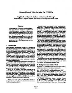
Fig. 1. An example of how the MEC quotient is constructed. By a, r we denote that the action a yields a reward of r.
b is defined as follows. Let sb ∈ Sb be some state in – the transition function ∆ the quotient and (s, a) ∈ Av(b s) an action available in sb. Then X ∆(s, a, s′ ) if sb′ = sbj , ′ ∈T ′ s b j ∆(b s, (s, a), sb ) = ∆(s, a, sb′ ) otherwise, i.e. sb′ ∈ S \ MECS .
For the sake of readability, we omit the added self-loop transitions of the form ∆(b si , (s, a), sbi ) with s ∈ Ti and a ∈ Ai from all figures. c s), we define rb(s, (s, a)) = r(s, a). b (s, a) ∈ Av(b – Finally, for sb ∈ S,
Furthermore, we refer to sb1 , . . . , sbn as collapsed states and identify them with the corresponding MECs.
b = ({s2 }, {a}), B b = Example 1. Figure 1a shows an MDP with three MECs, A b = ({s5 , s6 }, {a})). Its MEC quotient is shown in Figure 1b. △ ({s3 , s4 }, {a}), C
Remark 1. In general, the MEC quotient does not induce a DAG-structure, since there might be probabilistic transitions between MECs. Consider for example the MDP obtained by setting ∆(s2 , b, s4 ) = {s1 7→ 12 , s2 7→ 21 } in the MDP of b A, b (s2 , b)) = {s1 7→ 1 , B b 7→ 1 }. Figure 1a. Its MEC quotient then has ∆( 2 2
Remark 2. The MEC decomposition of an MDP M, i.e. the computation of MEC(M), can be achieved in polynomial time [CY95]. For improved algorithms on general MDPs and various special cases see [CH11,CH12,CH14,CL13]. Definition 3 (MEC restricted MDP). Let M be an MDP and (T, A) ∈ MEC(M) a MEC of M. By picking some initial state s′init ∈ T , we obtain the restricted MDP M′ = (T, s′init , A, Av′ , ∆′ , r′ ) where – Av′ (s) = Av(s) ∩ A for s ∈ T , – ∆′ (s, a, s′ ) = ∆(s, a, s′ ) for s, s′ ∈ T , a ∈ A, and – r′ (s, a) = r(s, a) for s ∈ T , a ∈ A. 6
Classification of MDPs If for some MDP M, (S, Act ) is a MEC, we call the MDP strongly connected. If it contains a single MEC plus potentially some transient states, it is called (weakly) communicating. Otherwise, it is called multichain [Put94, Sect. 8.3]. For a Markov chain, let ∆n (s, s′ ) denote the probability of going from the state s to state s′ in n steps. The period p of a pair s, s′ is the greatest common divisor of all n’s with ∆n (s, s′ ) > 0. The pair s, s′ is called periodic if p > 1 and aperiodic otherwise. A Markov chain is called aperiodic if all pairs s, s′ are aperiodic, otherwise the chain is called periodic. Similarly, an MDP is called aperiodic if every memoryless randomized strategy induces an aperiodic Markov chain, otherwise the MDP is called periodic. Long-run average reward In this work, we consider the (maximum) long-run average reward (or mean-payoff ) of an MDP, which intuitively describes the (maximum) average reward per step we expect to see when simulating the MDP for time going to infinity. Formally, let Ri be a random variable, which for an infinite path ρ = s0 a0 s1 a1 . . . returns Ri (ρ) = r(si , ai ), i.e. the reward observed at step i ≥ 0. Given a strategy π, the n-step average reward then is ! n−1 1X π π Ri , vn (s) := Es n i=0 and the long-run average reward of the strategy π is v π (s) := lim inf vnπ . n→∞
The lim inf is used in the definition, since the limit may not exist in general for an arbitrary strategy. Nevertheless, for finite MDPs the optimal limit-inferior (also called the value) is attained by some memoryless deterministic strategy π ∗ ∈ Π MD and is in fact the limit [Put94, Thm. 8.1.2]. ! n−1 X ∗ 1 v(s) := sup lim inf Eπs Ri = sup v π (s) = max v π (s) = lim vnπ . MD n→∞ n→∞ n π∈Π π∈Π π∈Π i=0 An alternative well-known characterization we use in this paper is X v(s) = max Pπs [♦�M ] · v(M ), π∈Π MD
(1)
M∈MEC
where ♦�M denotes the set of paths that eventually remain forever within M and v(M ) is the unique value achievable in the MDP restricted to the MEC M . Note that v(M ) does not depend on the initial state chosen for the restriction.
3 3.1
Value Iteration Solutions Naive value iteration
Value iteration is a dynamic-programming technique applicable in many contexts. It is based on the idea of repetitively updating an approximation of the 7
Algorithm 1 ValueIteration Input: MDP M = (S, sinit , Act , Av, ∆, r), precision ε > 0 Output: w, s.t. |w − v(sinit )| < ε 1: t0 (·) ← 0, n ← 0. 2: while stopping criterion not met do 3: n← n+1 4: for s ∈ S do � P 5: tn (s) = maxa∈Av(s) r(s, a) + s′ ∈S ∆(s, a, s′ )tn−1 (s′ ) 6: return
1 t (s ) n n init
value for each state using the previous approximates until the outcome is precise enough. The standard value iteration for average reward [Put94, Sect. 8.5.1] is shown in Algorithm 1. First, the algorithm sets t0 (s) = 0 for every s ∈ S. Then, in the inner loop, the value tn is computed from the value of tn−1 by choosing the action which maximizes the expected reward plus successor values. This way, tn in fact describes the optimal expected n-step total reward ! n−1 X π Ri = n · max vnπ (s). tn (s) = max Es π∈Π MD
π∈Π MD
i=0
Moreover, tn approximates the n-multiple of the long-run average reward Theorem 1 ([Put94, Thm. 9.4.1]). For any MDP M and any s ∈ S we have limn→∞ n1 tn (s) = v(s) for tn obtained by Algorithm 1. Stopping criteria The convergence property of Theorem 1 is not enough to make the algorithm practical, since it is not known when to stop the approximation process in general. For this reason, we discuss stopping criteria which describe when it is safe to do so. More precisely, for a chosen ε > 0 the stopping criterion guarantees that when it is met, we can provide a value w that is ε-close to the average reward v(sinit ). We recall a stopping criterion for communicating MDPs defined and proven correct in [Put94, Sect. 9.5.3]. Note that in a communicating MDP, all states have the same average reward, which we simply denote by v. For ease of notation, we enumerate the states of the MDP S = {s1 , . . . , sn } and treat the function tn as a vector of values tn = (tn (s1 ), . . . , tn (sn )). Further, we define the relative difference of the value iteration iterates as ∆n := tn − tn−1 and introduce the span semi-norm, which is defined as the difference between the maximum and minimum element of a vector w sp(w) = max w(s) − min w(s). s∈S
s∈S
The stopping criterion then is given by the condition sp(∆n ) < ε. 8
(SC1)
0.9 b, 0.9 · α
a, 0
0.1
s0
s1
a, α
b, 0 Fig. 2. A communicating MDP parametrized by the value α.
When the criterion (SC1) is satisfied we have that |∆n (s) − v| < ε
∀s ∈ S.
(2)
Moreover, we know that for communicating aperiodic MDPs the criterion (SC1) is satisfied after finitely many steps of Algorithm 1 [Put94, Thm. 8.5.2]. Furthermore, periodic MDPs can be transformed into aperiodic without affecting the average reward. The transformation works by introducing a self-loop on each state and adapting the rewards accordingly [Put94, Sect. 8.5.4]. Although this transformation may slow down VI, convergence can now be guaranteed and we can obtain ε-optimal values for any communicating MDP. The intuition behind this stopping criterion can be explained as follows. When the computed span norm is small, ∆n contains nearly the same value in each component. This means that the difference between the expected (n − 1)step and n-step total reward is roughly the same in each state. Since in each state the n-step total reward is greedily optimized, there is no possibility of getting more than this difference per step. Unfortunately, this stopping criterion cannot be applied on general MDPs, as it relies on the fact that all states have the same value, which is not true in general. Consider for example the MDP of Figure 1a. There, we have that v(s5 ) = v(s6 ) = 10 but v(s3 ) = v(s4 ) = 5. In [Put94, Sect. 9.4.2], it is conjectured that the following criterion may be applicable to general MDPs: sp(∆n−1 ) − sp(∆n ) < ε.
(SC2)
This stopping criterion requires that the difference of spans becomes small enough. While investigating the problem, we also conjectured a slight variation: k∆n − ∆n−1 k∞ < ε,
(SC3)
where kwk∞ = maxs∈S w(s). Intuitively, both of these criteria try to extend the intuition of the communicating criterion to general MDPs, i.e. to require that in each state the reward gained per step stabilizes. Example 2 however demonstrates that neither (SC2) nor (SC3) is a valid stopping criterion. Example 2. Consider the (aperiodic communicating) MDP in Figure 2 with a parametrized reward value α ≥ 0. The optimal average reward is v = α. But the first three vectors computed by value iteration are t0 = (0, 0), t1 = (0.9 · 9
α, α), t2 = (1.8 · α, 2 · α). Thus, the values of ∆1 = ∆2 = (0.9 · α, α) coincide, which means that for every choice of ε both stopping criteria (SC2) and (SC3) are satisfied by the third iteration. However, by increasing the value of α we can make the difference between the average reward v and ∆2 arbitrary large, so no guarantee like in Equation (2) is possible. △ 3.2
Local value iteration
In order to remedy the lack of stopping criteria, we provide a modification of VI using MEC decomposition which is able to provide us with an ε-optimal result, utilizing the principle of Equation (1). The idea is that for each MEC we compute an ε-optimal value, then consider these values fixed and propagate them through the MDP quotient. Apart from providing a stopping criterion, this has another practical advantage. Observe that the naive algorithm updates all states of the model even if the approximation in a single MEC has not ε-converged. The same happens even when all MECs are already ε-converged and the values only need to propagate along the transient states. These additional updates of already ε-converged states may come at a high computational cost. Instead, our method adapts to the potentially very different speeds of convergence in each MEC. The propagation of the MEC values can be done efficiently by transforming the whole problem to a reachability instance on a modified version of the MEC quotient, which can be solved by, for instance, VI. We call this variant the weighted MEC quotient. To obtain this weighted quotient, we assume that we have already computed approximate values w(M ) of each MEC M . We then collapse the MECs as in the MEC quotient but furthermore introduce new states s+ and s− , which can be reached from each collapsed state by a special action stay with probabilities corresponding to the approximate value of the MEC. Intuitively, by taking this action the strategy decides to “stay” in this MEC and obtain the average reward of the MEC. Formally, we define the function f as the normalized approximated value, 1 w(Mi ), so that it takes values in i.e. for some MEC Mi we set f (ˆ si ) = rmax [0, 1]. Then, the probability of reaching s+ upon taking the stay action in sˆi is defined as f (ˆ si ) and dually the transition to s− is assigned 1 − f (ˆ si ) probability. If for example some MEC M had a value v(M ) = 23 rmax , we would have that ∆(ˆ s, stay, s+ ) = 23 . This way, we can interpret reaching s+ as obtaining the maximal possible reward, and reaching s− to obtaining no reward. With this intuition, we show in Theorem 2 that the problem of computing the average reward is reduced to computing the value of each MEC and determining the maximum probability of reaching the state s+ in the weighted MEC quotient. c ∆, c = (S, b sˆinit , Act, d Av, b rb) Definition 4 (Weighted MEC quotient). Let M be the MEC quotient of an MDP M and let MECSb = {ˆ s1 , . . . , sˆn } be the set of collapsed states. Further, let f : MECSb → [0, 1] be a function assigning a value to every collapsed state. We define the weighted MEC quotient of M and f as d ∪ {stay}, Avf , ∆f , rf ), where the MDP Mf = (S f , sfinit , Act 10
s1 (s1 , b) b A 6 10
0.999
(s2 , b) 4 10
(s1 , a) 0.001 b C
b B
1
5 10
5 10
s−
s+
b 7→ Fig. 3. The weighted quotient of the MDP in Figure 1a and function f = {A 4 b 7→ 5 , C b 7→ 10 }. Rewards and stay action labels omitted for readability. , B 10 10 10
– S f = Sb ∪ {s+ , s− }, – sfinit = sˆinit , – Avf is defined as b Avf (ˆ ∀ˆ s ∈ S. s) = f
(
c s) ∪ {stay} Av(ˆ
c s) Av(ˆ
if sˆ ∈ MECSb, otherwise,
f
Av (s+ ) = Av (s− ) = ∅,
– ∆f is defined as b a d \ {stay}. ∆f (ˆ b s, a ∀ˆ s ∈ S, ˆ ∈ Act s, a ˆ) = ∆(ˆ ˆ)
∀ˆ si ∈ MECSb. ∆f (ˆ si , stay) = {s+ 7→ f (ˆ si , s− 7→ 1 − f (ˆ si )},
– and the reward function rf (ˆ s, a ˆ) is chosen arbitrarily (e.g. 0 everywhere), since we only consider a reachability problem on Mf . Example 3. Consider the MDP in Figure 1a. The average rewards of the MECs b 7→ 4, B b 7→ 5, C b 7→ 10}. With f defined as in Theorem 2, Figure 3 are v = {A shows the weighted MEC quotient Mf . △
Theorem 2. Given an MDP M with MECs MEC(M) = {M1 , . . . , Mn }, define 1 f (ˆ si ) = rmax v(Mi ) the function mapping each MEC Mi to its value. Moreover, f let M be the weighted MEC quotient of M and f . Then v(sinit ) = rmax · sup PπMf ,sf (♦s+ ). π∈Π
init
The corresponding algorithm is shown in Algorithm 2. It takes an MDP and the required precision ε as input and returns a value w, which is ε-close to the average reward v(sinit ). In the first part, for each MEC M the algorithm computes an approximate average reward w(M ) and assigns it to the function f (normalized by rmax ). Every MEC is a communicating MDP, therefore the value w(M ) can be computed using the naive VI with (SC1) as the stopping criterion. In the second part, the weighted MEC quotient of M and f is constructed and the maximum probability p of reaching s+ in Mf is approximated. 11
Algorithm 2 LocalVI Input: MDP M = (S, sinit , Act , Av, ∆, r), precision ε > 0 Output: w, s.t. |w − v(sinit )| < ε 1: f = ∅ 2: for Mi = (Ti , Ai ) ∈ MEC(M) do ⊲ Determine values for MECs 3: Compute the average reward w(Mi ) on M , such that |w(Mi ) − v(Mi )| < 12 ε, 1 4: f (ˆ si ) ← rmax w(Mi ) 5: Mf ← the weighted MEC quotient of M and f 1 6: Compute p s.t. |p − supπ∈Π PπMf ,sf (♦s+ )| < 2rmax ε init 7: return rmax · p
⊲ Determine reachability
Theorem 3. For every MDP M and ε > 0, Algorithm 2 terminates and is correct, i.e. returns a value w, s.t. |w − v(sinit )| < ε. ε For the correctness, we require that p is 2rmax -close to the real maximum probability of reaching s+ . This can be achieved by using the VI algorithms for reachability from [BCC+ 14a] or [HM14], which guarantee error bounds on the computed probability. Note that p can also be computed by other methods, such as linear programming. In Section 4 we empirically compare these approaches.
3.3
On-demand value iteration
Observe that in Algorithm 2, the approximations for all MECs are equally precise, irrespective of the effect a MEC’s value has on the overall value of the MDP. Moreover, the whole model is stored in memory and all the MECs are computed beforehand, which can be expensive for large MDPs. Often this is unnecessary, as we illustrate in the following example. b B, b C b in the MDP of Figure 1a. FurtherExample 4. There are three MECs A, π b more, we have that Psinit (♦C) ≤ 0.001. By using the intuition of Equation (1), we see that no matter where in the interval [0, rmax = 20] its value lies, it contributes to the overall value v(sinit ) at most by 0.001·rmax = 0.02. If the required b would precision were ε = 0.1, the effort invested in computing the value of C b not pay off at all and one can completely omit constructing C. b was a more complicated MEC, but after a few itFurther, suppose that A b is at most 4.4. erations the criterion (SC1) already shows that the value of A b b is greater Similarly, after several iterations in B, we might see that the value of B than 4.5. In this situation, there is no point in further approximating the value b since the action b leading to it will not be optimal anyway, and its precise of A value will not be reflected in the result. △
To eliminate these inefficient updates, we employ the methodology of bounded real-time dynamic programming (BRTDP) [MLG05] adapted to the undiscounted setting in [BCC+ 14a]. The word bounded refers to keeping and updating both a lower and an upper bound on the final result. It has been shown in [Put94,CI14] that bounds for the value of a MEC can be derived from the current maximum 12
and minimum of the approximations of VI. The idea of the BRTDP approach is to perform updates not repetitively for all states in a fixed order, but more often on the more important states. Technically, finite runs of the system are sampled, and updates to the bounds are propagated only along the states of the current run. Since successors are sampled according to the transition probabilities, the frequently visited (and thus updated) states are those with high probability of being reached, and therefore also having more impact on the result. In order to guarantee convergence, the non-determinism is resolved by taking the most promising action, i.e. the one with the current highest upper bound. Intuitively, when after subsequent updates such an action turns out to be worse than hoped for, its upper bound decreases and a more promising action is chosen next time. Since BRTDP of [BCC+ 14a] is developed only for MDP with the reachability (and LTL) objective, we decompose our problem into a reachability and MEC analysis part. In order to avoid pre-computation of all MECs with the same precision, we instead compute the values for each MEC only when they could influence the long-run average reward starting from the initial state. Intuitively, the more a particular MEC is encountered while sampling, the more it is “reached” and the more precise information we require about its value. To achieve this, we store upper and lower bounds on its value in the functions u and l and refine them on demand by applying VI. We modify the definition of the weighted MEC quotient to incorporate these lower and upper bounds by introducing the state s? (in addition to s+ , s− ). We call this construction the bounded MEC quotient. Intuitively, the probability of reaching s+ from a collapsed state now represents the lower bound on its value, while the probability of reaching s? describes the gap between the upper and lower bound. c ∆, c = (S, b sˆinit , Act, d Av, b rb) be Definition 5 (Bounded MEC quotient). Let M the MEC quotient of an MDP M with collapsed states MECSb = {ˆ s1 , . . . , sˆn } and let l, u : {ˆ s1 , . . . , sˆn } → [0, 1] be functions that assign a lower and upper bound, c The bounded MEC quotient Ml,u respectively, to every collapsed state in M. of M and l, u is defined as in Definition 4 with the following changes. – S l,u = Sb ∪ {s? }, – Avl,u (s? ) = ∅, – ∀ˆ s ∈ MECSb. ∆l,u (ˆ s, stay) = {s+ 7→ l(ˆ s), s− 7→ 1 − u(ˆ s), s? 7→ u(ˆ s) − l(ˆ s)}.
The unshortened definition can be found in Appendix D. The probability of reaching s+ and the probability of reaching {s+ , s? } give the lower and upper bound on the value v(sinit ), respectively. Corollary 1. Let M be an MDP and l, u functions mapping each MEC Mi of M to (normalized) lower and upper bounds on the value, respectively, i.e. 1 l(ˆ si ) ≤ rmax v(Mi ) ≤ u(ˆ si ). Then rmax · sup PπMl,u ,sl,u (♦s+ ) ≤ v(sinit ) ≤ rmax · sup PπMl,u ,sl,u (♦{s+ , s? }), π∈Π
init
π∈Π
where Ml,u is the bounded MEC quotient of M and l, u. 13
init
Algorithm 3 OnDemandVI Input: MDP M = (S, sinit , Act , Av, ∆, r), precision ε > 0, threshold k ≥ 2 Output: w, s.t. |w − v(sinit )| < ε 1: Set u(·, ·) ← 1, u(s− , ·) ← 0; l(·, ·) ← 0, l(s+ , ·) ← 1 ⊲ Initialize 2: Let A(s) := arg maxa∈Avl,u (s) u(s, a) 3: Let u(s) := maxa∈A(s) u(s, a) and l(s) := maxa∈A(s) l(s, a) 4: repeat 5: s ← sl,u ⊲ Generate path init , w ← s 6: repeat 7: a ← sampled uniformly from A(s) 8: s ← sampled according to ∆l,u (s, a) 9: w ← w, a, s 10: until s ∈ {s+ , s− , s? } or Appear(s, w) = k ⊲ Terminate path 11: if pop(w) = s? then ⊲ Refine MEC in which stay was taken 12: pop(w) 13: qb ← top(w) 14: Run VI on qb, updating u and l, until u − l is halved 15: Update ∆l,u (b q , stay) according to Definition 5 16: else if Appear(s, w) = k then ⊲ Update EC-collapsing 17: OnTheFlyEc 18: repeat ⊲ Back-propagate values 19: a ← pop(w), s ← pop(w) P 20: u(s, a) ←P s′ ∈S ∆(s, a, s′ ) · u(s′ ) 21: l(s, a) ← s′ ∈S ∆(s, a, s′ ) · l(s′ ) 22: until w = ∅ 2ε 23: until u(sinit ) − l(sinit ) < rmax ⊲ Terminate 1 24: return rmax · 2 (u(sinit ) + l(sinit))
Algorithm 3 shows the on-demand VI. The implementation maintains a partial model of the MDP and Ml,u , which contains only the states explored by the runs. It interleaves two concepts: (i) naive VI is used to provide upper and lower bounds on the value of discovered end components, (ii) the method of [BCC+ 14a] is used to compute the reachability on the collapsed MDP. In lines 6–10 a random run is sampled following the “most promising” actions, i.e. the ones with maximal upper bound. The run terminates once it reaches s+ , s− or s? , which only happens if stay was one of the most promising actions. A likely arrival to s? reflects a high difference between the upper and lower bound and, if the run ends up in s? , this indicates that the upper and lower bounds of the MEC probably have to be refined. Therefore, in lines 11–15 the algorithm resumes VI on the corresponding MEC to get a more precise result. This decreases the gap between the upper and lower bound for the corresponding collapsed state, thus decreasing the probability of reaching s? again. The algorithm uses the function Appear(s, w) = |{i ∈ N | s = w[i]}| to count the number of occurrences of the state s on the path w. Whenever we encounter the same state k times (where k is given as a parameter), this indicates that the run may have got stuck in an end component. In such a case, the algorithm 14
Procedure 4 OnTheFlyEc 1: for (Ti , Ai ) ∈ MEC(Ml,u ) do 2: Collapse (Ti , Ai ) to sˆi in Ml,u 3: for s ∈ Ti , a ∈ Av(s) \ Ai do 4: u(ˆ si , (s, a)) ← u(s, a) 5: l(ˆ si , (s, a)) ← l(s, a) 6: Add the stay action according to Definition 5.
calls OnTheFlyEc [BCC+ 14a], presented in Procedure 4, to detect and collapse end components of the partial model. By calling OnTheFlyEc we compute the bounded quotient of the MDP on the fly. Without collapsing the end components, our reachability method could remain forever in an end component, and thus never reach s+ , s− or s? . Finally, in lines 18–22 we back-propagate the upper and lower bounds along the states of the simulation run. Theorem 4. For every MDP M, ε > 0 and k ≥ 2, Algorithm 3 terminates almost surely and is correct, i.e. returns a value w, s.t. |w − v(sinit )| < ε.
4
Implementation and experimental results
In this section, we compare the runtime of our presented approaches to established tools. All benchmarks have been run on a 4.4.3-gentoo x64 virtual machine with 3.0 GHz per core, a time limit of one hour and memory limit of 8GB. The precision requirement for all approximative methods is ε = 10−6 . We implemented our constructions as a package in the PRISM Model Checker [KNP11]. We used the 64-bit Oracle JDK version 1.8.0 102-b14 as Java runtime for all executions. All measurements are given in seconds, measuring the total user CPU time of the PRISM process using the UNIX tool time. 4.1
Models
First, we briefly explain the examples used for evaluation. virus [KNPV09] models a virus spreading through a network. We reward each attack carried out by an infected machine. Note that in this model, no machine can “purge” the virus, hence eventually all machines will be infected. cs nfail [KPC12] models a clientserver mutual exclusion protocol with probabilistic failures of the clients. A reward is given for each successfully handled connection. investor [MM07,MM02] models an investor operating in a stock market. The investor can decide to sell his stocks and keep their value as a reward or hold them and wait to see how the market evolves. The rewards correspond to the value of the stocks when the investor decides to sell them, so maximizing the average reward corresponds to maximizing the expected selling value of the stocks. phil nofair [DFP04] represents the (randomised) dining philosophers without fairness assumptions. We use two reward structures, one where a reward is granted each time a philosopher “thinks” or “eats”, respectively. rabin [Rab82] is a well-known mutual 15
exclusion protocol, where multiple processes repeatedly try to access a shared critical section. Each time a process successfully enters the critical section, a reward is given. zeroconf [KNPS06] is a network protocol designed to assign IP addresses to clients without the need of a central server while still avoiding address conflicts. We explain the reward assignment in the corresponding result section. sensor [KPC12] models a network of sensors sending values to a central processor over a lossy connection. A reward is granted for every work transition. 4.2
Tools
We will compare several different variants of our implementations, which are described in the following. – Naive value iteration (NVI) runs the value iteration on the whole MDP as in Algorithm 1 of Section 3.1 together with the stopping criterion (SC2) conjectured by [Put94, Sect. 9.4.2]. As the stopping criterion is incorrect, we will not only include the runtime until the stopping criterion is fulfilled, but also until the computed value is ε-close to the known solution. – Our MEC decomposition approach presented in Algorithm 2 of Section 3.2 is denoted by MEC-reach , where reach identifies one of the following reachability solver used on the quotient MDP. • PRISM’s value iteration (VI), which iterates until none of the values change by more than 10−8 . While this method is theoretically imprecise, we did not observe this behaviour in our examples.4 • An exact reachability solver based on linear programming (LP) [Gir14]. • The BRTDP solver with guaranteed precision of [BCC+ 14a] (BRTDP). This solver is highly configurable. Among others, one can specify the heuristic which is used to resolve probabilistic transitions in the simulation. This can happen according to transition probability (PR), roundrobin (RR) or maximal difference (MD). Due to space constraints, we only compare to the MD exploration heuristic here. Results on the other heuristics can be found in Appendix E. – ODV is the implementation of the on-demand value iteration as in Algorithm 3 of Section 3.3. Analogously to the above, we only provide results on the MD heuristic here. The results on ODV together with the other heuristics can also be found in Appendix E. Furthermore, we will compare our methods to the state-of-the-art tool MultiGain, version 1.0.2 [BCFK15] abbreviated by MG. MultiGain uses linear programming to exactly solve mean payoff objectives among others. We use the commercial LP solver Gurobi 7.0.1 as backend5 . We also instantiated reach by an implementation of the interval iteration algorithm presented in [HM14]. This variant performed comparable to MEC-VI and therefore we omitted it. 4
5
PRISM contains several other methods to solve reachability, which all are imprecise and behaved comparably in our tests. MultiGain also supports usage of the LP solver lp solve 5.5 bundled with PRISM, which consistently performed worse than the Gurobi backend.
16
Table 1. Runtime comparison of our approaches to MultiGain on various, reasonably sized models. Timeouts (1h) are denoted by TO. Strongly connected models are denoted by “scon” in the MEC column. The best result in each row is marked in bold, excluding NVI due to its imprecisions. For NVI, we list both the time until the stopping criterion is satisfied and until the values actually converged. Model
States MECs
virus cs nfail4 investor phil-nofair5 rabin4
809 960 6688 93068 668836
4.3
MG
NVI
1 3.76 3.50/3.71 176 4.86 10.2/TO 837 16.75 4.23/TO scon TO 23.5/30.3 scon TO 87.8/164
MEC-VI 4.09 4.38 8.83 70 820
MEC-LP MEC-BRTDP 4.41 TO TO 70 820
4.40 9.39 64.5 70 820
ODV TO 16.0 18.7 TO TO
Results
The experiments outlined in Table 1 show that our methods outperform MultiGain significantly on most of the tested models. Furthermore, we want to highlight the investor model to demonstrate the advantage of MEC-VI over MEC-LP. With higher number of MECs in the initial MDP, which is linked to the size of the reachability LP, the runtime of MEC-LP tends to increase drastically, while MEC-VI performs quite well. Additionally, we see that NVI fails to obtain correct results on any of these examples. ODV does not perform too well in these tests, which is primarily due to the significant overhead incurred by building the partial model dynamically. This is especially noticeable for strongly connected models like phil-nofair and rabin. For these models, every state has to be explored and ODV does a lot of superfluous computations until the model has been explored fully. On virus, the bad performance is due to the special topology of the model, which obstructs the back-propagation of values. Moreover, on the two strongly connected models all MEC decomposition based methods perform worse than naive value iteration as they have to obtain the MEC decomposition first. Furthermore, all three of those methods need the same amount of for these models, as the weighted MEC quotient only has a single state (and the two special states), thus the reachability query is trivial. In Table 2 we present results of some of our methods on zeroconf and sensors, which both have a structure better suited towards ODV. The zeroconf model consists of a big transient part and a lot of “final” states, i.e. states which only have a single self-loop. sensors contains a lot of small, often unlikely-tobe-reached MECs. On the zeroconf model, we evaluate the average reward problem with two reward structures. In the default case, we assign a reward of 1 to every final state and zero elsewhere. This effectively is solving the reachability question and thus it is not surprising that our method gives similarly good results as the BRTDP solver of [BCC+ 14a]. The avoid evaluation has the reward values flipped, i.e. all states except the final ones yield a payoff of 1. With this reward assignment, the algorithm performed slightly slower, but still extremely fast given the size of the 17
Table 2. Runtime comparison of our on-demand VI method with the previous approaches. All of those behaved comparable to MEC-VI or worse, and due to space constraints we omit them. MO denotes a memory-out. Aside from runtime, we furthermore list the number of explored states and MECs of ODV Model zeroconf(40,10) avoid zeroconf(300,15) avoid sensors(2) sensors(3)
States
MEC-VI
ODV
ODV States
ODV MECs
3001911
MO
5.05
4730203
MO
16.6
7860 77766
18.9 2293
20.1 37.2
481 582 873 5434 3281 10941
3 3 3 3 917 2301
model. We also tried assigning pseudo-random rewards to every non-final state, which did not influence the speed of convergence noticeably. We want to highlight that the mem-out of MEC-VI already occurred during the MEC-decomposition phase. Hence, no variant of our decomposition approach can solve this problem. Interestingly, the naive value iteration actually converges on zeroconf (40,10) in roughly 20 minutes. Unfortunately, as in the previous experiments, the used incorrect stopping criterion was met a long time before that. Further, when comparing sensors(2) to sensors(3), the runtime of ODV only doubled, while the number of states in the model increased by an order of magnitude and the runtime of MEC-VI even increased by two orders of magnitude. These results show that for some models, ODV is able to obtain an ε-optimal estimate of the mean payoff while only exploring a tiny fraction of the state space. This allows us to solve many problems which previously were intractable simply due to an enormous state space.
5
Conclusion
We have discussed the use of value iteration for computing long-run average rewards in general MDPs. We have shown that the conjectured stopping criterion from literature is not valid, designed two modified versions of the algorithm and have shown guarantees on their results. The first one relies on decomposition into VI for long-run average on separate MECs and VI for reachability on the resulting quotient, achieving global error bounds from the two local stopping criteria. The second one additionally is simulation-guided in the BRTDP style, and is an anytime algorithm with a stopping criterion. The benchmarks show that depending on the topology, one or the other may be more efficient, and both outperform the existing linear programming on all larger models. For future work, we pose the question of how to automatically fine-tune the parameters of the algorithms to get the best performance. For instance, the precision increase in each further call of VI on a MEC could be driven by the current values of VI on the quotient, instead of just halving them. This may reduce the number of unnecessary updates while still achieving an increase in precision useful for the global result. 18
References [BBC+ 14] Tom´ aˇs Br´ azdil, V´ aclav Broˇzek, Krishnendu Chatterjee, Vojtˇech Forejt, and Anton´ın Kuˇcera. Two views on multiple mean-payoff objectives in Markov decision processes. LMCS, 10(1), 2014. [BCC+ 14a] Tom´ as Br´ azdil, Krishnendu Chatterjee, Martin Chmelik, Vojtech Forejt, Jan Kret´ınsk´ y, Marta Z. Kwiatkowska, David Parker, and Mateusz Ujma. Verification of Markov decision processes using learning algorithms. In ATVA, pages 98–114. Springer, 2014. [BCC+ 14b] Tom´ as Br´ azdil, Krishnendu Chatterjee, Martin Chmelik, Vojtech Forejt, Jan Kret´ınsk´ y, Marta Z. Kwiatkowska, David Parker, and Mateusz Ujma. Verification of markov decision processes using learning algorithms. CoRR, abs/1402.2967, 2014. [BCFK13] Tom´ as Br´ azdil, Krishnendu Chatterjee, Vojtech Forejt, and Anton´ın Kucera. Trading performance for stability in Markov decision processes. In LICS, pages 331–340, 2013. [BCFK15] Tom´ as Br´ azdil, Krishnendu Chatterjee, Vojtech Forejt, and Anton´ın Kucera. MultiGain: A controller synthesis tool for MDPs with multiple mean-payoff objectives. In TACAS, pages 181–187, 2015. [BFRR14] V. Bruy`ere, E. Filiot, M. Randour, and J-F. Raskin. Meet your expectations with guarantees: Beyond worst-case synthesis in quantitative games. In STACS’14, pages 199–213, 2014. [BK08] Christel Baier and Joost-Pieter Katoen. Principles of model checking, 2008. [CH11] Krishnendu Chatterjee and Monika Henzinger. Faster and dynamic algorithms for maximal end-component decomposition and related graph problems in probabilistic verification. In SODA, pages 1318–1336. SIAM, 2011. [CH12] Krishnendu Chatterjee and Monika Henzinger. An O(n 2 ) time algorithm for alternating b¨ uchi games. In SODA, pages 1386–1399. SIAM, 2012. [CH14] Krishnendu Chatterjee and Monika Henzinger. Efficient and dynamic algorithms for alternating b¨ uchi games and maximal end-component decomposition. J. ACM, 61(3):15:1–15:40, 2014. [Cha07] Krishnendu Chatterjee. Markov decision processes with multiple long-run average objectives. In FSTTCS, pages 473–484, 2007. [CI14] Krishnendu Chatterjee and Rasmus Ibsen-Jensen. The complexity of ergodic mean-payoff games. In ICALP, Part II, volume 8573 of Lecture Notes in Computer Science, pages 122–133. Springer, 2014. [CKK15] Krishnendu Chatterjee, Zuzana Kom´ arkov´ a, and Jan Kret´ınsk´ y. Unifying two views on multiple mean-payoff objectives in markov decision processes. In LICS, pages 244–256, 2015. [CL13] Krishnendu Chatterjee and Jakub Lacki. Faster algorithms for Markov decision processes with low treewidth. In CAV, Proceedings, pages 543– 558, 2013. [CR15] Lorenzo Clemente and Jean-Francois Raskin. Multidimensional beyond worst-case and almost-sure problems for mean-payoff objectives. In LICS, pages 257–268, 2015. [CY95] Costas Courcoubetis and Mihalis Yannakakis. The complexity of probabilistic verification. J. ACM, 42(4):857–907, 1995. [dA97] Luca de Alfaro. Formal verification of probabilistic systems. PhD thesis, Stanford University, 1997.
19
[DFP04]
M. Duflot, L. Fribourg, and C. Picaronny. Randomized dining philosophers without fairness assumption. Distributed Computing, 17(1):65–76, 2004. [FKR95] J.A. Filar, D. Krass, and K.W Ross. Percentile performance criteria for limiting average Markov decision processes. Automatic Control, IEEE Transactions on, 40(1):2–10, Jan 1995. [FV97] Jerzy Filar and Koos Vrieze. Competitive Markov decision processes. Springer-Verlag, 1997. [Gir14] Sergio Giro. Optimal schedulers vs optimal bases: An approach for efficient exact solving of markov decision processes. Theor. Comput. Sci., 538:70– 83, 2014. [HM14] Serge Haddad and Benjamin Monmege. Reachability in MDPs: Refining convergence of value iteration. In International Workshop on Reachability Problems, pages 125–137. Springer, 2014. [How60] Ronald A. Howard. Dynamic programming and Markov processes. The MIT press, New York London, Cambridge, MA, 1960. [KNP11] M. Kwiatkowska, G. Norman, and D. Parker. PRISM 4.0: Verification of probabilistic real-time systems. In G. Gopalakrishnan and S. Qadeer, editors, CAV, volume 6806 of LNCS, pages 585–591. Springer, 2011. [KNPS06] M. Kwiatkowska, G. Norman, D. Parker, and J. Sproston. Performance analysis of probabilistic timed automata using digital clocks. Formal Methods in System Design, 29:33–78, 2006. [KNPV09] Marta Kwiatkowska, Gethin Norman, David Parker, and Maria Grazia Vigliotti. Probabilistic mobile ambients. Theoretical Computer Science, 410(12-13):1272–1303, 2009. [KNS03] Marta Kwiatkowska, Gethin Norman, and Jeremy Sproston. Probabilistic model checking of deadline properties in the ieee 1394 firewire root contention protocol. Formal Aspects of Computing, 14(3):295–318, 2003. [KPC12] Anvesh Komuravelli, Corina S P˘ as˘ areanu, and Edmund M Clarke. Assumeguarantee abstraction refinement for probabilistic systems. In International Conference on Computer Aided Verification, pages 310–326. Springer, 2012. [MLG05] H. Brendan McMahan, Maxim Likhachev, and Geoffrey J. Gordon. Bounded real-time dynamic programming: RTDP with monotone upper bounds and performance guarantees. In ICML, pages 569–576, 2005. [MM02] A. McIver and C. Morgan. Games, probability and the quantitative mucalculus qmu. In M. Baaz and A. Voronkov, editors, Proc. LPAR’02, volume 2514 of LNAI. Springer, 2002. [MM07] A. McIver and C. Morgan. Results on the quantitative mu-calculus qMu. ACM Transactions on Computational Logic, 8(1), 2007. [PGT03] Joelle Pineau, Geoffrey J. Gordon, and Sebastian Thrun. Point-based value iteration: An anytime algorithm for pomdps. In IJCAI, pages 1025–1032, 2003. [Put94] M.L. Puterman. Markov decision processes: Discrete stochastic dynamic programming. John Wiley and Sons, 1994. [Rab82] Michael O Rabin. N-process mutual exclusion with bounded waiting by 4· log2n-valued shared variable. Journal of Computer and System Sciences, 25(1):66–75, 1982. [RRS15] Mickael Randour, Jean-Fran¸cois Raskin, and Ocan Sankur. Percentile queries in multi-dimensional markov decision processes. In CAV 2015, Proceedings, Part I, pages 123–139, 2015. [Seg95] R. Segala. Modelling and Verification of Randomized Distributed Real Time Systems. PhD thesis, Massachusetts Institute of Technology, 1995.
20
[Vei66]
Arthur F. Veinott. On finding optimal policies in discrete dynamic programming with no discounting. Ann. Math. Statist., 37(5):1284–1294, 10 1966. [WBB+ 10] Ralf Wimmer, Bettina Braitling, Bernd Becker, Ernst Moritz Hahn, Pepijn Crouzen, Holger Hermanns, Abhishek Dhama, and Oliver E. Theel. Symblicit calculation of long-run averages for concurrent probabilistic systems. In QEST, pages 27–36, 2010.
Appendix A
Proof of Theorem 2
We use ,S to denote the event of reaching some state in S in the next step. X PπM,sinit (♦�Mi ) · v(Mi ) v(sinit ) = sup π∈Π
Mi ∈MEC(M)
= rmax · sup π∈Π
X
si ) PπM,sinit (♦�Mi ) · f (ˆ
Mi ∈MEC(M)
(since v(Mi ) = rmax · f (ˆ si ) by assumption) X π si ∧ , (s+ ∨ s− ))) · f (ˆ si ) PMf ,sf (♦ (ˆ = rmax · sup π∈Π
= rmax · sup π∈Π
init
Mi ∈MEC(M)
X
si ) · PπMf ,ˆsi (,(s+ ∨ s− )) · f (ˆ si ) PπMf ,sf (♦ˆ init
Mi inMEC(M)
(by the Markov property) X si ) · PπMf ,ˆsi (,s+ ) PπMf ,sf (♦ˆ = rmax · sup π∈Π
init
Mi ∈MEC(M)
(since PπMf ,ˆsi (,s+ ) = PπMf ,ˆsi (,(s+ ∨ s− )) · f (ˆ si ))
= rmax · sup PπMf (♦s+ ).
⊓ ⊔
π∈Π
21
B
Proof of Theorem 3
Algorithm 2 terminates since every part only takes finitely many steps. We now prove correctness, i.e. that upon termination the algorithm returns value p, such that |rmax · p − v(sinit )| < ε. X si ) PπM,sinit (♦�Mi ) · f (ˆ sup PπMf ,sf (♦s+ ) = sup init
π∈Π
π∈Π
Mi ∈MEC(M)
(from the proof of Theorem 2) X v(Mi ) + 12 ε PπM (♦�Mi ) ≤ sup rmax π∈Π
(by assumption)
Mi ∈MEC(M)
=
≤ =
1
rmax 1 rmax
· sup π∈Π
X
PπM,sinit (♦�Mi ) · v(Mi ) + 21 ε
Mi ∈MEC(M)
1 ε + sup 2
π∈Π
X
Mi ∈MEC(M)
ε v(sinit ) + . rmax 2rmax
PπM,sinit (♦�Mi ) · v(Mi )
Analogously we can prove that supπ∈Π PπMf ,sf (♦s+ ) ≥ init
v(sinit ) ε rmax − 2rmax .
sup Pπ f f (♦s+ ) − v(sinit ) ≤ ε π∈Π M ,sinit rmax 2rmax
By assumption it also holds that p − sup Pπ f f (♦s+ ) < M ,s π∈Π
init
�
ε 2rmax
By the triangle inequality we obtain from (3) and (4) that p − v(sinit ) < ε . rmax rmax
Together (3)
(4)
and thus
|rmax · p − v(sinit )| < ε.
C
⊓ ⊔
Proof of Theorem 4
We extend the proof of [BCC+ 14a, Thm. 3], which can be found in the technical report [BCC+ 14b]. To this end, we summarize some properties of u and l. Let M be some MEC and sˆi its corresponding collapsed state. – u(ˆ si ) and l(ˆ si ) are always and upper and lower bound of value of M . This follows from the error bound on VI within M . 22
– Let ni be the number of times the stay action is taken in sˆi . We have lim (u(ˆ si ) − l(ˆ si )) = 0.
ni →∞
This follows from convergence of VI on MECs and by the fact that if stay is taken infinitely often, a round of VI on M happens infinitely often. Consequently, the proof of [BCC+ 14b, Thm. 3] applies.
D
⊓ ⊔
Definition of bounded MEC quotient
c ∆, c = (S, b sˆinit , Act, d Av, b rb) Definition 6 (Bounded MEC quotient). Let M be the MEC quotient of an MDP M with collapsed states MECSb = {ˆ s1 , . . . , sˆn }. Further, let l, u : {ˆ s1 , . . . , sˆn } → [0, 1] be functions assigning a lower and upper bound, respectively, to every collapsed state. We define the bounded MEC quol,u l,u l,u d tient of M and f as the MDP Ml,u = (S l,u , sl,u init , Act ∪ {stay}, Av , ∆ , r ), where – S l,u = Sb ∪ {s+ , s− , s? }, – sl,u ˆinit , init = s l,u – Av is defined as b Av ∀ˆ s ∈ S. Av
l,u
l,u
(ˆ s) =
(
c s) ∪ {stay} Av(ˆ c s) Av(ˆ
(s+ ) = Av
l,u
(s− ) = Av
if sˆ ∈ MECSb, otherwise, l,u
(s? ) = ∅,
– ∆l,u is defined as c s) \ {stay}. ∆l,u (ˆ b a b s, a ∀ˆ s ∈ S, ˆ ∈ Av(ˆ s, a ˆ) = ∆(ˆ ˆ)
∀ˆ s ∈ MECSb. ∆l,u (ˆ s, stay) = {s+ 7→ l(ˆ s), s− 7→ 1 − u(ˆ s), s? 7→ u(ˆ s) − l(ˆ s)}, – and the reward function rl,u (ˆ s, a ˆ) is chosen arbitrarily (e.g. 0 everywhere), since we only consider a reachability problem on Ml,u .
E
More experimental data
23
Table 3. Additional data for Table 1. The results for MEC-BRTDP and ODV using the different heuristics are listed in the order PR, RR, MD Model
States MECs
virus 809 cs nfail4 960 investor 6688 phil-nofair5 93068 rabin4 668836
1 176 837 scon scon
MEC-BRTDP
ODV
4.69/3.96/4.40 20.3/8.83/9.39 47.1/48.6/64.5 70 820
TO/2452/TO 51.3/15.4/16.0 17.3/21.3/18.7 TO/TO/TO TO/TO/TO
Table 4. Additional data for Table 2. We listed the results of using ODV with the three different mentioned exploration heuristics. Heuristics are listed in the order PR, RR, MD Model
States
zeroconf(40,10) 3001911 avoid zeroconf(300,15) 4730203 avoid sensors(2) 7860 sensors(3) 77766
Time
Explored States
83.4/9.72/5.05 1831/294/16.6 31.8/26.1/20.1 305/480/37
24
Explored MECs
516/1643/481 3/3/3 905/2475/582 3/3/3 731/2291/873 3/3/3 1595/10759/5434 3/22/3 5308/4915/3281 1474/1444/917 31431/34239/10941 9125/11041/2301