Value Prediction in Engineering Applications G. Ziegler1 , Z. Palotai2 , T. Cinkler1 , P. Arat´ o2 , and A. L˝ orincz3 1
Budapest University of Technology and Economics, Department of Telecommunication and Telematics High Speed Networks Laboratory, http://hsnlab.ttt.bme.hu mailto:
[email protected] 2 Budapest University of Technology and Economics, Department of Control Engineering and Information Technology http://www.iit.bme.hu/nwelcome.html 3 E¨ otv¨ os Lor´ and University, Department of Information Systems, Neural Information Processing Group, http://valerie.inf.elte.hu/˜lorincz/ Budapest, Hungary
Abstract. In engineering application heuristics are widely used for discrete optimization tasks. We report two cases (in Dense Wavelength Division Multiplexing and High Level Synthesis), where a recent “intelligent” heuristic (STAGE) performs excellently by learning a value-function of the states. We have found that if a global structure of local minima is found by the function approximator then search time may not have to scale with the dimension of the problem in the exponent, but it may become a polynomial function of the dimension.
1
Introduction
One of the most fundamental activities in an engineer’s life is to find good, probably the best (i.e., optimal ) choice of different alternatives in situations offering many alternatives while respecting certain limitations. Given a problem one usually evaluates the possibilities according to some strategy and finally selects one, which seems optimal for him. In engineering the problem of finding the best possible answer from a large space of possible answers is called global optimization. Formally speaking a global optimization task consists of the following tuples: a state space X together with a scalar objective function Obj : X → R used for assessing the states. Our goal is to find the “best” state x∗ ∈ X, which minimizes1 Obj, that is, Obj(x∗ ) ≤ Obj(x) ∀x ∈ X. If the state space is small, then x∗ can be trivially obtained by exhaustive search, otherwise special knowledge or some heuristics have to be utilized for performing effective partial search [1]. Many practical combinatorial optimization problems in engineering where X is finite, but enormous in size fall into the class of NP-Hard problems [2], to which no efficient exact solution algorithm is known. One possibly adapts the solution algorithm according to his best knowledge in order to incorporate his special “insights” regarding the problem. The main 1
In the followings when we speak about optimization, we will always assume minimization, unless explicitly noted.
L. Monostori, J. V´ ancza, and M. Ali (Eds.): IEA/AIE 2001, LNAI 2070, pp. 25–34, 2001. c Springer-Verlag Berlin Heidelberg 2001
26
G. Ziegler et al.
problem comes from the fact that the true nature of the problem can be very well hidden behind the objective function, therefore searching only by objective function can be very inefficient. In the theory of Reinforcement Learning [3] the fundamental instrument in decision making is the so called evaluation function, or shortly value function. It maps features of a given state to a single scalar value that gives us the “promise of the state” with respect to the solution to the problem. [4]. Obtaining this mapping is not a straightforward task. The good news is that evaluation functions can be learnt automatically [3], [4]. In the subsequent section we shortly overview the details of a recent algorithm called STAGE. In the main part of our paper we will report our experience that value prediction can indeed help to find either better results, or similar results but faster and more reliably than the widely used original heuristics.
2
Global Optimization with Value Prediction: STAGE
As we discussed in Section 1, if exhaustive search is not feasible one can resort to local search (LS). There is a big number of heuristics used for improving the chance of the LS to find global optimum, the interested reader is kindly referred to [1]. Performing local search requires the definition of the neighborhood structure N , which gives a set of states that is considered to be reachable directly (i.e., locally) from current state x. The definition of N can strongly influence the effectiveness of LS. STAGE [4] falls into the class of multiple-restart heuristics and exploits the fact that the result of a LS might be strongly dependent on the start point of the search. The “value” of a state equals to the likely outcome of the LS starting from that state. Using this promise as an evaluation function STAGE performs “intelligent” restarts by searching the state with the most promising value. The values of the states are produced by a function approximator (FAPP) via a userdefined scalar “feature” vector F that should grasp the main attributes of the problem. STAGE works cyclically, it repeatedly performs two LS-s consecutively. Firstly the LS πloc defined by the user is run. It should produce a finite trajectory used for retraining the FAPP. Secondly STAGE starts another LS independent from the one that was used for searching by Obj to find the state x b∗ with the ∗ ∗ b as the re-start point best value estimate, i.e., Vb (b x ) ≤ Vb (x) ∀x ∈ X. It uses x for its next cycle. STAGE highly benefits from using this approach. On one hand it allows the user to freely replace the input with a few selected feature. On the other hand, using FAPP opens the door before generalization (inter- and extrapolation). If there is a trend toward the global optimum among local optima then this trend can be learnt by the FAPP dramatically boosting the efficiency of STAGE. The precise details of STAGE is beyond the length-limits of this paper, it can be found in [4].
Value Prediction in Engineering Applications
3
27
Joint Multilayer Configuration of GMPLS Networks
3.1
Problem Overview
In DWDM (Dense Wavelength Division Multiplexing) optical telecommunication networks [5] an end-to-end optical channel routed over several network nodes can be established. This is referred to as WR (Wavelength Routing). Unfortunately, for networks consisting of N nodes N (N − 1) unidirectional light-paths are needed (N (N − 1)/2 pairs), which number depends on the square of N . Wavelength conversion does not help much. For this reason Multi-hop WR is used, i.e., two or more traffic streams can be carried jointly, over a single lightpath by multiplexing and demultiplexing of these traffic streams in time division manner (it is called “grooming”). Therefore, electrical (de-)multiplexer devices are needed. Recently introduced GMPLS (Generalized Multi-Protocol Label Switching) networks use packet switching over WR-DWDM networks handling several network layers jointly over a single control plane2 [6]. Although GMPLS signalling will allow configuring all the layers on demand, at the moment it seems to be most reasonable to re-configure the layers rarely. Following this approach here we propose a novel model for joint configuration of the GMPLS layers. This model allows use of heuristic optimization methods like STAGE and other techniques. To make the presentation easier, the result on an example network is depicted in Fig. 1. The drawing shows the given six-node (N1-N6) network. The nodes are interconnected by seven physical links (L1-L7). In this example we assume three different wavelengths WL1, WL2 and WL3 and we assume that all nodepairs wish to communicate. There are 15 traffic streams between the node-pairs and 25 so-called Basic Building Units (BBUs 1-25). A BBU defines the assigned wavelength of a given stream on a given link. With the given physical topology we obtain 15 initial light-paths using 15 hops where opto-electrical and electrooptical conversions were needed. Seven of length one (4;8;10;12;14;18;22) six of length two (2-9;3-7;5-11;13-21;15-24;19-23) and two of length three (1-6-16;17-2520). The minimal necessary four hops remained after optimization are denoted by small circles in Fig. 1. We first route the traffic demands over the physical network then we search for an optimal wavelength assignment for each traffic demands over each physical links. We cut the paths between node-pairs into sequences and merge the sequences into so called λ-links, assigning them the same wavelength across consecutive physical links along the path. The problem size grows rapidly with the number of nodes and the number of available wavelengths. This problem very likely belongs to the class of NP-hard problems, because the subproblem of it, the Static Light-path Establishment (SLE) has been shown to be NP-complete [7]. Already in the example given in Fig. 1 with six nodes, three available wavelengths and 25 BBUs the state space consists of 325 different states. The problem 2
Packet Switching Layer, Time-Division Multiplexing Layer, Lambda(Wavelength)Switching Layer and Fiber-Switching Layer
28
G. Ziegler et al. L1
N1
L3
L2
1 2 3 4 5
9 10
L4
N2 11 12 13
18 19 20
L6
N4 WL1
N3
6 7 8 L5
14 15 16 17
21 22 23 24 25
N5
L7
WL2
N6 WL3
Fig. 1. The optimal configuration of the example
will be significantly reduced if the state space is tightened by starting with assigning one and the same wavelength to all traffic streams between adjacent nodes (i.e., of length one ). 3.2
Reformulating the Problem for STAGE
For solving the GMPLS configuration problem with STAGE we have to define the building blocks of the STAGE algorithm. Beyond πloc we need a second LS algorithm to find the extremum of the estimated values over the feature-space. We follow the suggestion of [4] and we use quadratic regression as FAPP, and Stochastic Hill-Climber to search in the feature space. The X problem space is defined by the possible allocations of wavelengths to BBU-s. The Obj to be minimized is the number of electro-optical conversions, that is, the sum of the number of wavelength-conversion and the number of multiplexing and de-multiplexing of different traffics to–from the same wavelength at some node. The neighborhood structure N is defined by the allowed configuration actions: changing the wavelength of one BBU. As for features several metrics can be defined. STAGE can automatically select from the features. The effect of irrelevant features will be simply noise and they will be integrated out by the FAPP. From the tried features finally the most successful ones have been chosen, namely the loads of the individual wavelengths (how many traffic demands have been carried over a particular wavelength) and the distribution factor of loads over all wavelengths. This experience is in correlation with the statement of [4] that using only a few, coarse feature of the problem is usually the most efficient solution. 3.3
Performance of STAGE on the GMPLS Problem
We have tested the following local searches [8]: Hill-Climber with equi-cost moves (HC) and Simulated Annealing (SA), each with and without smart restarts (SR). The networks have been the 6-node one of Figure 1 using 3 wavelengths (problem ‘A’), and a bigger 10-node one using 3 and 5 wavelengths (problems ‘B’ and ‘C’, respectively), see Table 1.
Value Prediction in Engineering Applications
29
Table 1. Comparison of GMPLS optimization results w. and w/o. SR
SR—Smart Restart, HC—Hill–Climb., SA—Sim.Anneal., BestObj—best Obj., #best—no. of visited states with BestObj, #visited—tot. no. of visited states, Obj gain—BestObj gain of SR over non-SR
Firstly the non-SR algorithms were run. We have tried different settings to determine the upper limit of trajectory length where no further significant improvement was probable. Experience has shown that the FAPP usually stabilized after ten retrain cycles, so in the SR mode we have cut-back the permitted trajectory length of πloc to one tenth. It has resulted in having the same total number of visited states for both SR and non-SR modes (around 73000). We have found that for smaller problems the STAGE approach has not improved significantly the obtained results. However, as the problem size has grown STAGE has begun to excel in robustness3 . Note the table rows separated by dashed lines in Table 1. Each these dual rows contains data for SR runs of the same problem. Rows immediately above dashed lines contain the number of occurrences of those states where the Obj is at least as good as the best one in the non-SR runs of the same problem instance. SR runs have yielded appr. the same quality results with the same number of visited states as the non-SR runs, but with a robustness usually better by more than one order of magnitude. In the following section we will turn to another engineering problem instance, where the SR approach has also helped to get better results than earlier algorithms.
3
We call robustness the number of visited states with the best Obj versus the total number of states visited.
30
4
G. Ziegler et al.
High Level Synthesis Design Problem
Our design problem is a high–level synthesis (HLS) problem: register transfer level (RTL) hardware description is to be given from a task formulated at a higher level [9], [10]. We compare the performance of STAGE with graph–coloring heuristics see, e.g.,[2] and with the state–of–the–art heuristics, DECIP [11]. Our methodology allows the joint optimization of software and hardware components. In general, the first step of any kind of design is to determine the components that will not be decomposed any further. We shall call such components extended elementary components, or extended elementary operations (EO-s, see [12]). The word ‘extended’ is added to emphasize that the algorithms we utilize are not limited to addition, subtraction, and multiplication, but higher order units, such as FFT, ciphering, etc. units can be considered as EO-s. Restrictions on the properties of EO-s define the type of design under consideration. Combinatorial explosion of the design phase deprives the direct translation of HLS description into layout at more complex design tasks. Therefore, we rely on using elements that can perform different operations, called Intellectual Property (IP, see [13], [14]). The method described here can be extended to pipelined operations. The HLS problem has been formulated for this novel class. In turn, the method can deal with pipelining IP-s as sub–units [15]. We are interested in the so called “allocation problem”, which determines which EO will be executed by which IP. One should try to schedule the EO-s as early as possible (potentially requiring parallel, or pipe-lined operation of several IP-s). On the other we have to allocate processors (IP-s) for each EO using as few IP as possible. The optimization problem is known to be NP–complete (see, e.g., [9] and references therein). We will show that allocation can be transcribed into a generalized “satisfiability” problem of CNF formulae. Assigning cost to each clause of the CNF, the sum of the individual costs of unsatisfied clauses constitutes the total cost of the CNF, which is to be minimized. The novelty of our approach is in the “transcription”. Our transcription allows the incorporation of any solution derived by heuristics, a major advantage for future steps. Our method is general enough to take into account constraints (inequalities), biases (cost components), and heuristics (suboptimal policies) in the global search procedure. 4.1
Allocation as a Weighted CNF Problem
We have reformulated the above mentioned allocation problem as a special binary satisfiability problem. The set of EO-s that the ith IP is capable of executing (‘compatible’) is denoted by Ri , i = 1, . . . , n. The so-called maximum compatibility classes are formed by those EO-s that can be safely allocated to one IP (for formal details please refer to [9]) are denoted by Mk , k = 1, . . . , κ. The TCNF reformulation starts with creating variables. Let us denote the set {Ri Mk | 0 ≤ i ≤ n, 1 ≤ k ≤ κ} by mi,k and call these sets allocation sets. To each set mi,k there belongs a binary variable ti,k . The variable can take values ‘true’ and ‘false’. The value of the ti,k variable is ‘true’ provided that the EO-s belonging to set mi,k are allocated to the ith IP, Πi .
Value Prediction in Engineering Applications
31
Next we create the so called unused clauses (UC-s). The negated values of the variables will be included into our CNF. These are trivial clauses. This type of clause is called ‘unused compatibility clause’ or shortly, UC clause. The name denotes that a ‘true’ UC clause means that the compatibility class of the clause is not used. Later cost will be rendered to the UC clauses. Finally we create the so called EO clauses. EO clauses express the conditions that each EO should be allocated. The number of EO clauses is equal to the number of EO-s. In each EO clause the possible allocations of that EO are listed with ’OR’ relations in between. An allocation in allocation set mi,κ is possible if the set contains the EO under consideration. If an EO clause is true then the EO is allocated. Our listing concerns only compatible allocations. In turn, if every EO clause is true then every EO is allocated. The CNF expression is created by making the disjunctions of the conjunctions. In turn, the allocation problem is transformed into a CNF expression. 4.2
Turning CNF into a Minimization Problem for STAGE
We note, that in our formulation a solution of the design problem is ‘found’ if all of the variables are set to value ‘true’. This solution, however, can be very expensive. This is so, because we are using every UC clause instead of using as few as necessary. In what follows we will derail from traditional solutions to CNFs. Costs will be assigned to each clause. The task will be the minimization of the cumulated costs. This formulation fits the philosophy of the STAGE algorithm. We shall make restrictions on the costs in order to force the algorithm to find solutions. The state space X is trivial: the boolean variables Ti,k . Two CNF states are considered neighbors (N ) if they differ in the value of a single variable. We use WalkSat [16], a highly efficient search algorithm as the local policy of STAGE. The change of the value of a variable is possible provided that the cost of the CNF is decreasing. If this is not the case but at least one state with identical cost is found then one of these states is selected with predefined probability. The design of the cost structure is of crucial importance. In our design we have included variables and clauses and fabricated the cost of those to ensure that any local search provides a solution. Such solutions can be, however, very costly. The underlying structure of the cost, however, can be discovered by STAGE. Details of the cost structure can be found elsewhere [15]. A quadratic approximator served as a FAPP (see Section 2). Features were chosen as follows: (i) Obj(x), (ii) the number of clauses that can be satisfied by a single variable, (iii) the number of clauses that can be satisfied by two variables, (iv) the number of variables that make a clause of the actual CNF ’false’ if inverted and, (v) the number of ’spurious’ variables. (A variable is called ’spurious’ if the number of its normal occurrences in the CNF is larger than the number of its negated occurrences.) 4.3
Computational Results
Allocation problems were tested on several realistic problems. To any design problem these parameters, e.g., the cost of the IP, or the time of execution can
32
G. Ziegler et al. Table 2. Overview of results for different problems
Problem Name Cosine equation Sine expansion 12 point FFT
Number of Cost of the problem Number Number of variables Number of types Restart compatibility in the CNF Graph DECIP STAGE of EO-s of IP-s time sets formulae Coloring 8 14 10 8 56 58 58 58 30 11 54 58 50 50 16 6 31 24 56 80 76 72 49 52 103 56 48 40 64 93 174 36 40 32 180 180 36 6 14 180 302 180 34 941 832 120 108 96
be chosen according to the designers data. Tests were started by running PIPE with its internal graph-coloring procedure. Compatibility classes were generated at this step. Compatibility classes were used in DECIP. The same compatibility classes were used for STAGE. Time requirements of the computer runs are illustrative; different computer languages were used for the different algorithms — depending on the flexibility and time requirements of the different sub–problems. Communication between optimization routines was automated when it was desired. Parameters of STAGE were ’tweaked’ experimentally on small problems [15]. Tested examples included cosine theorem; a 5 term Taylor–expansion of sine function and a 12 point Fast Fourier Transformation with different scheduling parameters (restart times). The dimension of the search space (the ’size’) of the individual problems and the computational results are summarized in Table 2. Local search times are shown in the inset diagram of Fig. 2 with respect to problem size (which equals to ‘No. of EO-s’ * ‘No. of IP-s’ * ‘No. of compatibility classes’. DECIP has three parameters that weight relative costs. One cycle of DECIP corresponds to one choice of parameter vectors. DECIP was computed for an exhaustive search of 125 parameter combinations. This exhaustive search for DECIP was made for the sake of safety in the comparison. According to our computer simulations STAGE with FAPP-s are ideal to speed–up the search in the parameter space of DECIP too. In the case of STAGE one cycle consists of a local search and the search for intelligent restart. Graph-coloring is not shown in these figures. Graph coloring was much faster than the two other algorithms, however, it has produced relatively poor results.
5
Closing Remarks
We have found that function approximator based estimation of the value function is advantageous in two engineering applications, in Dense Wavelength Division Multiplexing and in High Level Synthesis. It is important that if global structure is found by the function approximator then search time may not have to scale with the dimension of the problem in the exponent, but it may become a polynomial function of the dimension. We underline this point by a comparison
Value Prediction in Engineering Applications
33
Time (sec)
10000
100000
1000
100
STAGE DECIP
10
CPU Time of solution in seconds
10000
1 0
1 0 000
1000
20000
3 0 000
40000
500 0 0
Problem size
100
10
1
0.1
0.01 80 50
100 50
170 50
300 50
160 100
200 100
340 100
600 100
320 200
400 200
680 200
1200 200
Top row: number of clause, Bottom row: number of variables ILP Best time
ILP Worst time
STAGE Best time
STAGE Worst time
Fig. 2. Inset diagram: Experienced running time versus problem size, main diagram: Comparison of CPLEX and Stage
between CPLEX (a commercially available ILP solver) and STAGE. Comparisons between running times for different CNF-s are shown in the main diagram of Fig. 2. A trend can observed that ‘intelligent restart’ can be, indeed, intelligent. This is the reason that the relative performance of STAGE is improving by problem complexity. (CPU strength was was better by about a factor of five for CPLEX.) Finally we note that there is no known algorithm for designing features. This problem is left for the designer and requires experience. It is an intriguing question whether the design of features can be automated. From the theoretical point of view, the question is to find higher order descriptors or non-linear transformations for a given problem that diminish the number of local maxima stopping local search procedures. Transcription of this sentence to reward, e.g., by considering the distance traveled by the local search procedure and the improvement of the cost achieved allows one to formulate the search problem for features that could make use of function approximators. This point, however, remains to be seen.
34
G. Ziegler et al.
References 1. D. P. Bertsekas. Network Optimization: Continuous and Discrete Models. Optimization and Neural Computation Series. Athena Scientific, Belmont, Massachusetts, 1998. 2. Editor D.S. Hochbaum. Approximation Algorithms for NP-Hard Problems. PWS Publishing Co., Boston, 1995. 3. R. S. Sutton and A. G. Barto. Reinforcement learning: An introduction. MIT Pess, 1998. 4. Justin Andrew Boyan. Learning Evaluation Functions for Global Optimization. PhD dissertation, School of Computer Science, Carnegie Mellon University, Pittsburgh PA 15213, August 1998. 5. K.N. Sivarajan R. Ramaswami. Routing and wavelength assignment in all-optical networks. IEEE Transactions on Networking, 3(5):489–500, Oct. 1995. 6. P. Ashwood-Smith. Generalized mpls - signalling functional description. http://www.ietf.org/internet-drafts/. 7. I. Chlamtac, A. Ganz, and G. Karmi. Lightpath communications: An approach to high bandwidth optical WANs. IEEE Transactions on Communications, 40(7):1171–1182, July 1992. 8. Tibor Cinkler. Heuristic algorithms for configuration of the ATM-layer over optical networks. In Proceedings of the ICC‘97, IEEE International Conference on Communications, Montr´ eal, pages 1164–1168, June 1997. 9. P. Arat´ o, I. Jankovits, S. Szigeti, and T. Visegr´ ady. High-level Synthesis of Pipelined Datapaths. PANEM, Budapest, 1999. 10. R. Camposano and W. Rosenstiel. Synthetizing circuits from behavioural descriptions. IEEE Transactions on Computer Aided Design, pages 171–180, 1989. 11. P. Arat´ o, T. Kand´ ar, Z. Mohr, and T. Visegr´ ady. An algorithm for decomposition into predefined IP-s. Technical report, Technical University of Budapest, 2000. 12. G. DeMicheli. Synthesis and Optimization of Digital Circuits. McGraw Hill, 1994. 13. J. Staunstrup and W. Wolf (eds). Hardware/Software Codesign: Principles and Practice. Kluwer Academic Publisher, 1997. 14. Rolf Ernst. Embedded System Architectures, System Level Synthesis, volume 357 of Nato Science Series. Kluwer Academic Publisher, 1999. Edited by A.A. Jerraya and J. Mermet. 15. Z. Palotai and A. L˝ orincz. Joint optimization of scheduling and allocation of IPs. manuscript in preparation. 16. B. Selman, H. A. Kautz, and B. Cohen. Local search strategies for satisfiability testing. Second DIMACS Challenge on Cliques, Coloring and Satisfiability, pages 44, 95–96, 1996.