Valuing Options in Regime-Switching Models
Nicolas P.B. Bollen†
ABSTRACT This paper presents a lattice-based method for valuing both European and American-style options in regime-switching models. The Black-Scholes model is shown to generate significant pricing errors when a regime-switching process governs underlying asset returns. In addition, regime-switching option values are shown to generate implied volatility smiles commonly found in empirical studies. These results provide encouraging evidence that the valuation technique is important, and rich enough to capture salient features of traded option prices.
Current Version: January 29, 1998
†
Assistant Professor, Eccles School of Business, University of Utah, Salt Lake City, Utah 84112. E-mail
[email protected]. The author gratefully acknowledges the comments of Stephen Gray and Robert Whaley, as well as seminar participants at Duke, Indiana, and Southern Methodist Universities and the Universities of Iowa and Utah.
Valuing Options in Regime-Switching Models
Regime-switching models effectively capture the complex time series properties of several important financial variables, including interest rates and exchange rates. Existing research develops the econometrics of regime-switching models and demonstrates their advantages over other models. However, option valuation in a regime-switching framework has received little attention. This paper presents a lattice-based method for valuing both European and American-style options in regimeswitching models. The Black-Scholes model is shown to generate significant pricing errors when a regime-switching process governs underlying asset returns. In addition, regime-switching option values are shown to generate implied volatility smiles commonly found in empirical studies. These results provide encouraging evidence that the valuation technique is important, and rich enough to capture salient features of traded option prices. The intuition behind regime-switching models is clear: as economic environments change, so do the data generating processes of related financial variables. One example is the U.S. short-term interest rate. For much of the past 25 years, the volatility of the short rate has been relatively low. Occasionally, however, there have been sudden switches to periods of extremely high volatility. The causes of these regime switches have been varied. The Federal Reserve experimented with monetary policy from 1979 to 1982. The result was high interest rate volatility for the duration of the experiment. Other periods of high volatility coincided with changes in the economic and political environments due to war, the OPEC oil crisis, and the October 1987 stock market crash (see Hamilton (1990) and Gray (1996)). In other words, the short-term interest rate appears to switch between high and low volatility regimes in response to changes in macroeconomic and political factors. Regime-switching models seek to capture such discrete shifts in the behavior of financial variables by allowing the parameters of the underlying data-generating process to take on different values in different time periods. Past research develops econometric methods for estimating parameters in regime-switching models, and demonstrates how regime-switching models can characterize the time series behavior of some variables better than existing single-regime models. Hamilton (1990) studies a regime-switching model with constant moments in each regime. He constructs and maximizes a loglikelihood function based on the probability of switching regimes to estimate parameters. Hamilton (1994) and Gray (1995) simplify the estimation by reformulating the problem in terms of the probability 1
of being in a particular regime, conditional on observable information. Gray’s framework also explicitly allows for conditional transition probabilities and time-varying moments within each regime. Gray (1996) offers a study of interest rates and shows that a regime-switching model provides better volatility forecasts than either a constant-variance or a single-regime GARCH model. His result implies that accurate option valuation may require the specification of a regime-switching process for some underlying asset returns, since volatility forecasts are the key input to all derivative valuation methods. Much research has been devoted to developing lattice methods for representing stochastic processes for use in option valuation. Cox, Ross, and Rubinstein (1979) show how a simple binomial lattice can accurately represent geometric Brownian motion. Boyle (1988) and Boyle, Evnine, and Gibbs (1989) construct more elaborate lattices to accommodate several stochastic variables. Hull and White (1990) show how to model linear mean reversion and a particular form of conditional heteroskedasticity in a lattice. None of the existing lattices, however, can be used to represent a regime-switching model. This paper develops a lattice for valuing both European and American-style options in regimeswitching models. Five branches are used at each node to match the mean and variance of each regime and to improve the efficiency of the lattice. The accuracy of the lattice is demonstrated using Monte Carlo simulation. The Black-Scholes model is shown to result in significant pricing errors when a regime-switching process governs underlying asset returns. In addition, regime-switching option values are shown to generate implied volatility smiles commonly found in empirical work. These results indicate that option valuation in regime-switching models has practical relevance for investors. The plan for the rest of the paper is as follows. The following section discusses regimeswitching models and their implications for option valuation. Section 2 introduces a pentanomial lattice that approximates a regime-switching process. Section 3 describes how to value options using the pentanomial lattice. Section 4 presents some numerical examples. The last section concludes.
2
1. Regime-Switching Models
Most financial models concerning a stochastic variable such as an interest rate, exchange rate, or a stock price specify the distribution from which changes in the variable are drawn. For example, the familiar geometric Brownian motion used in the Black-Scholes (1973) model of stock prices implies that continuously compounded returns are normally distributed:
b g
r ~ N µ,σ .
(1)
Unfortunately, empirical studies have found little evidence supporting simple, stationary distributions in financial models. Sample moments are easily shown to vary through time. One approach to this problem is to consider additional sources of uncertainty, such as stochastic volatility used in the large family of GARCH models. Regime-switching models add even greater flexibility by allowing the parameters of the stochastic variable’s distribution to take on different values in different regimes. For ease of exposition, this paper considers a two-regime model in which returns are normally distributed in both regimes. At any point in time, the particular regime from which the next observation is drawn is unobservable and denoted by the latent indicator variable St. However, one can infer the probability that each regime will govern the next observation, as shown in Hamilton (1994) and Gray (1996). Let pi,t denote the probability that regime i will govern the observation recorded at time t. Also, let Φt-1 denote the information set used to determine pi,t. The two-regime model can be expressed as: rt | Φ t −1 ~
RS N (µ ,σ ) with probability T N (µ ,σ ) with probability 1
1
0
0
p1,t 1 − p1,t ,
(2)
where
b
g
p1,t = Pr St = 1| Φ t −1 .
(3)
Central to the statistical analysis of regime-switching models is the process that governs switches between regimes. Transition probabilities, also naturally referred to as regime persistence parameters, are the probabilities of staying in either regime from one observation to the next. The standard regime-switching model of Hamilton (1990) uses constant transition probabilities. Gray (1996) introduces a generalized regime-switching model (GRS) which can condition transition probabilities on the history of the data under investigation. One example of a variable that might have time-varying transition probabilities is a foreign exchange rate. Suppose that government intervention 3
in the foreign exchange market is more likely when one currency has appreciated or depreciated substantially versus another. This relation can be modeled by a function linking the probability of switching regimes to the level of the exchange rate. Again, for ease of exposition I focus on the simpler case, although the numerical methods introduced later in the paper can also be used in a GRS setting. In a two-regime model, two transition probabilities are required. Let χ denote the persistence of regime 1:
c
h
c
h
χ = Pr St = 1 St −1 = 1 ,
(4)
and let ψ denote the persistence of regime 0: ψ = Pr St = 0 St −1 = 0 .
(5)
The persistence of regimes affects the relation between successive regime probabilities. Using Bayesian conditioning arguments, Gray (1996) shows that p1,t is related to prior regime probabilities as follows: p1,t = χ
LM Ng
OP b Q
g1,t −1 p1,t −1 + 1−ψ 1,t −1 p1,t −1 + g 0 ,t −1 p0,t −1
gLMM g N
c
h OP, p PQ
g0,t −1 1 − p1,t −1 p
1,t −1 1,t −1
+ g 0 , t −1
(6)
0 , t −1
where
R| F S| GH T
1 1 rt − µ i gi,t = exp − 2 σi 2πσ i
IJ U|V. K |W 2
(7)
The relation between p0,t and prior regime probabilities is given by (6) except χ is replaced by (1-χ) and (1-ψ) is replaced by ψ. Regime-switching models complicate option valuation because neither the current nor the future distribution of underlying asset returns is known with certainty. Since the distribution of returns is uncertain, the problem of valuing options in regime-switching models bears similarities to option valuation with stochastic volatility. Several important contributions have been made in this area.1 Hull and White (1987), for example, show that under certain assumptions, the expected average volatility over the option’s life can be used in a closed-form solution for European-style option values. Naik (1993) uses a similar argument in a simplified regime-switching model. He also derives a closed-form solution for European-style option values. Naik’s solution involves the density of the time spent in a particular regime over the option’s life, and is conditional on the starting regime.
4
The approach taken in this paper is to construct a lattice that represents the possible future paths of a regime-switching variable. Option values are computed by forming expectations of their payoffs over the branches of the lattice. This discrete-time framework contributes in several ways. First, it allows for the valuation of both European and American-style options. Since trading volume for American-style options dominates in several important markets, such as currency options, the lattice approach makes a significant practical contribution. Second, it is flexible enough to incorporate transition probabilities that are arbitrary functions of the underlying asset and time. Third, it can incorporate uncertainty regarding the current regime. Finally, it is intuitive and easy to use.
2. Lattice Construction
This section shows how to construct a pentanomial lattice that approximates the evolution of a variable with returns governed by a regime-switching process. Subsection 2.1 reviews the traditional binomial lattice as a means of representing random changes in a variable governed by a single regime. Subsection 2.2 introduces a pentanomial lattice that allows for the simultaneous representation of two regimes. Subsection 2.3 discusses a technical issue regarding the impact of discretization in the lattice on regime transition probabilities.
2.1. The Binomial Lattice The binomial lattice of Cox, Ross, and Rubinstein (1979) approximates the evolution of a variable governed by geometric Brownian motion. This stochastic process implies that the variable’s continuously compounded returns over some discrete interval of time ∆t are normally distributed:
d
i
r ~ N µ∆ t , σ ∆ t ,
(8)
where µ and σ are the instantaneous mean and volatility of returns. The binomial lattice uses a two dimensional grid of nodes to represent the possible sequences of returns observed over a finite interval. At each node, the lattice approximates the normal distribution of the variable’s return over the next instant using a binomial distribution. The DeMoivre-Laplace theorem ensures that the discrete
1
See for example Hull and White (1987), Stein and Stein (1991), Heston (1993), Ball and Roma (1994).
5
distribution of the variable’s returns at the end of the lattice converges to the normal distribution implied by the stochastic process as the number of nodes in the lattice is made sufficiently large. Each node in a binomial lattice has two free parameters: the probability of traveling along the upper branch, denoted by π, and the continuously compounded rate of return of the variable after traveling along the upper branch, denoted by ∆φ. These parameters are chosen so that the first two moments of the variable’s return implied by the lattice match the first two moments implied by the underlying distribution. At the node level, two equations and two unknowns are relevant. The mean equation sets the expected return implied by the lattice equal to the distribution’s mean: πe ∆φ + (1 − π )e − ∆φ = e µ∆t .
(9)
The variance equation sets the variance implied by the lattice equal to the distribution’s variance: r
~
N
d
µ
∆
t , σ
∆
t
i,
(10)
These equations can be solved to yield the following values for π and ∆φ: e µ∆t − e − ∆φ π = ∆φ e − e − ∆φ
∆φ = σ 2 ∆t + µ 2 ∆t 2 .
(11)
Some simple algebra shows that the resulting probabilities lie between 0 and 1. After calculating the branch probabilities and the step size, one can construct a lattice to represent possible future paths followed by the variable.
2.2. The Pentanomial Lattice This subsection shows how to construct a pentanomial lattice that represents changes in a variable when returns are governed by a regime-switching process. The process has two regimes and constant within-regime means and variances, as specified in equation (2). The regime-switching lattice must match the moments implied by each regime’s distribution, and should reflect the regime uncertainty and switching possibilities of a regime-switching model. To develop intuition for the regime-switching lattice, let each node in a lattice represent the seed value of two binomial distributions, one for each regime. Two sets of two branches emanate from each node; I call this a quadranomial lattice. When both sets of branches are symmetric about a horizontal line passing through the seed node, the inner two branches always correspond to the regime with lower volatility. The step size and branch probabilities of each binomial lattice can be chosen to 6
match the moments of the corresponding regime’s distribution using the equations in (11). Each set of branch probabilities must now be interpreted as the branch probabilities conditional on being in a particular regime, hereafter referred to as the conditional branch probabilities. Although the quadranomial lattice accurately represents both distributions, its branches generally do not recombine efficiently. Unless the step size of the high volatility regime happens to be exactly twice that of the low volatility regime, the number of nodes at time step t will be t2. This exponential growth severely restricts the number of time steps available in the lattice, thereby limiting its ability to accurately approximate the underlying model. One way to address this problem is to add a fifth branch for the express purpose of enhancing the recombining properties of the lattice.2 The additional branch allows the regimes’ step sizes to be adjusted so that one is twice the other, while maintaining the match between the lattice moments and the distributions’ moments. In the five-branch “pentanomial” lattice, one of the regimes is represented by a trinomial at every node in the lattice. The other regime is represented by a binomial at every node in the lattice. The step size of the regime represented by the trinomial can be increased so that the step sizes of the two regimes are in a 1:2 ratio. The branch probabilities of the trinomial are calculated so that the first two moments implied by the lattice match the moments of the underlying distribution. The modified lattice now is a pentanomial, with four outer branches symmetric about the middle branch, and the branches evenly spaced. See figure 1 for an illustration. As illustrated in figure 2, branches of the evenly spaced pentanomial recombine more efficiently than the quadranomial, reducing the number of nodes at time step t from t2 to 4t - 3. As the number of time steps in the lattice increases, the efficiency gain from using a pentanomial lattice increases. As seen in table 1, for example, a 500-step tree requires a total of 41,791,750 nodes in a quadranomial lattice, but only 499,500 in a pentanomial lattice, a reduction of about 99%. To determine which regime is represented by the trinomial lattice, one first calculates the binomial lattice branch probabilities and step sizes for both regimes. The low volatility regime will use
2
Multiple branch lattices have been used to solve a variety of problems. Boyle (1988) uses a pentanomial lattice to value claims with two state variables. Boyle, Evnine, and Gibbs (1989) use an n-dimensional binomial lattice to model the joint evolution of several variables. Hull and White (1990) use a trinomial lattice to model mean reversion. I considered simpler lattice structures, such as a trinomial that represents both regimes, but the pentanomial is the only one that ensures non-negative branch probabilities.
7
the trinomial if its step size is less than one-half the step size of the high volatility regime, otherwise the high volatility regime will use the trinomial. Suppose, for example, that returns in the high volatility regime have a mean of 1% and a volatility of 5% per observation, and returns in the low volatility regime have a mean of -1% and a volatility of 1.5% per observation. Suppose also that the time step of the lattice equals the time between observations, so that ∆t = 1. Using equation (11) to determine the step sizes, ∆φh = .051 and ∆φl = .018, where the subscripts h and l indicate the high and low volatility regimes. Here the low volatility step size is less than one-half the high volatility step size, so the low volatility regime will be represented by the trinomial lattice. The conditional branch probabilities of the high volatility regime remain unchanged from the binomial results of equation (11), so the conditional probability of traveling along the high volatility regime’s upper branch is .586. The step size of the low volatility regime is set equal to one-half the step size of the high volatility regime, ∆φl = .025. Next, the three conditional branch probabilities of the low volatility regime are determined by matching the moments implied by the lattice to the moments implied by the distribution of the low volatility regime. For the low volatility regime, the mean equation is: π l ,u e ∆φ h 2 + π l ,me 0 + (1 − π l ,u − π l ,m )e − ∆φ h 2 = e µ l ∆t ,
(12)
where the subscripts u, m, and d denote the up, middle, and down branches. The corresponding variance equation is:
b
g
b
g
π l ,u ∆φ h 2 + (1 − π l ,u − π l ,m ) − ∆φ h 2 − µ l2 ∆t 2 = σ l2 ∆t . 2
2
(13)
The solutions to these two equations are: π l ,u =
e µ l ∆t − e − ∆φ h 2 − π l ,m (1 − e − ∆φ h 2 ) e ∆φ h 2 − e − ∆φ h 2
b
π l ,m = 1 − 4 ∆φ l ∆φ h
g
2
(14)
π l ,d = 1 − π l ,u − π l ,m , where both step sizes in equation (14) are from the binomial calculations. For the parameters of the numerical example, these three probabilities are .052, .500, and .448. It can be shown that for small enough ∆t, these probabilities will lie between 0 and 1. (Proof available from the author.) When the high volatility regime uses the trinomial, equations similar to (12) - (14) are constructed by setting the step size of the high volatility regime equal to twice that of the low volatility regime.
8
So far I have described the structure of the lattice and the probabilities associated with each branch, conditional on regime. Section 3 shows how to use the lattice to value options.
2.3. Discretization and Transition Probabilities The ability of a lattice to accurately represent a continuous distribution using discrete intervals can generally be improved by decreasing the duration of each interval. Standard processes such as geometric Brownian motion can be partitioned into arbitrarily fine time steps since observations are identically and independently distributed. The regime-switching model, however, specifies a relation between successive observations based on regime persistence. Since regime persistence is a function of the time between observations, it must be adjusted when decreasing the duration of steps in a lattice. Recall that a regime’s transition probability, or persistence, is defined as the probability of staying in the regime from one observation to the next. Regime persistence is clearly dependent on the time period between observations. Suppose the time between observations is halved. The new duration requires new persistence parameters. The relation between the two sets of persistence parameters can be established by equating regime persistence over the same interval using both sets of parameters. Let Χ denote the persistence of regime 1 and Ψ the persistence of regime 0 for the original time step. Let χ denote the persistence of regime 1 and ψ the persistence of regime 0 for the smaller time step. Two equations result: Χ = χ 2 + (1 − χ )(1 − ψ ) Ψ = ψ 2 + (1 − ψ )(1 − χ ).
(15)
The solution to these equations relates the two sets of persistence parameters as follows: ψ 2 + 1 − ψ − (1 − ψ ) ψ 2 + Χ − Ψ − Ψ = 0 χ = ψ 2 + Χ − Ψ.
(16)
Two values for ψ which straddle Ψ will solve the quadratic. The higher value is used, consistent with the inverse relation between regime persistence and the time between observations. The positive χ is used, consistent with the definition of a probability. Note that when the persistence parameters of two regimes are identical for the original time step, they are also identical for the shorter time step.
3. Option Valuation in the Lattice 9
Lattices are useful for valuing options because they approximate the probability distribution of future values of the underlying variable. Since option cash flows are functions of the value of the underlying asset, options can be valued in the lattice by taking the expectation of their payoffs. The current option value equals the discounted expected option payoff.
3.1. Risk-Neutral Valuation In the Black-Scholes (1973) model, risk-neutral valuation of options is appropriate since the differential equation that defines option value is independent of risk preferences. The implications of risk-neutrality for option valuation are that one can replace the drift of the underlying asset by the riskless rate, less any continuous dividend yield, and perform all discounting at the riskless rate. As discussed in section 1, regime-switching models add an element of stochastic volatility to the problem of option valuation. In this setting the traditional risk-neutrality argument breaks down. There are two ways to proceed. First, as in Hull and White (1987), one can assume that the additional risk of stochastic volatility is not priced in the market. Second, as in Naik (1993), one can apply a risk adjustment to the persistence parameters of a regime-switching model. For the purposes of this paper, I assume that “regime-risk” is not priced in the market so that risk-neutral valuation of options is appropriate. Thus the calculations of step sizes and branch probabilities in the lattice are made with regime means set to the riskless rate of interest, less any dividend yield. Furthermore, discounting occurs at the riskless rate.
3.2. Valuing Options in the Lattice In a binomial lattice representing a single-regime model, the terminal array of nodes gives a range of future values of the asset. Option cash flows at expiration are calculated as the maximum of zero and the exercise proceeds. The current option value is calculated by folding back to the beginning of the lattice. At each node, branch probabilities are used to calculate the expected option value in adjacent nodes. For American-style options, rational early exercise is checked at each node. The present value of the option is calculated at the seed node of the lattice. In a pentanomial lattice representing a regime-switching model, time-varying regime probabilities and the possibility of switching regimes at each node complicate computing expectations. 10
To simplify matters, two conditional option values are calculated at each node, where the conditioning information is the regime that governed the prior observation. Options are valued in the standard way, iterating backward from the terminal array of nodes. For the terminal array, the two conditional option values are the same at each node. They are simply the maximum of zero and the option’s exercise proceeds. For earlier nodes, conditional option values will depend on regime persistence since the persistence parameters are equivalent to future regime probabilities in a conditional setting. For example, suppose the lattice is used to value an American-style call option. The call option at time t, conditional on regime 1, is related to conditional option values at time t+1 as follows:
b g
c t ,1 = Max θ t − X , e
− r f ∆t
nχE cbt + 11, g + b1 − χ g E cbt + 1,0g s ,
(17)
where θt is the time t value of the asset, X is the exercise price of the option, and rf is the riskless rate of interest. The early exercise proceeds are compared to the discounted expected option value one period later. Regime 1’s persistence affects the expectation of future option value by weighting the expectations of future conditional option values. Expectations of the future conditional option values are taken over the appropriate regime’s branches using the corresponding conditional branch
b
g
, probabilities. In figure 1, for example, E c t + 11
b
g
E c t + 1,0
is computed over the outer two branches and
is computed over the inner three branches. Similarly, the call option at time t, conditional
on regime 0, is affected by regime 0’s persistence:
b
c ,0
Max θ t
X,
r f ∆t
nb1 ψ g E c
g
11 ,
b
ψE c
1,0
s.
(18)
In many situations, market participants have knowledge of the current regime. For example, if exchange rate regimes are defined by government policy, and policy announcements are credible, then
probabilities can be computed using Bayes’ Rule and the prior observations of the underlying variable, as shown in section 1. I conducted an experiment to determine the degree of certainty with which
experiment, regime 1 has weekly volatility of 3%, regime 0 has 1% weekly volatility, and regime means are both 5% annually. The initial regime probability is 50%, indicating no knowledge of the initial 11
regime. Four weeks of the underlying process were simulated over a range of regime persistence values and observation frequencies. The regime persistence is equal across regimes in all cases. Within each simulation, random regime switches were chosen consistent with the underlying persistence, observations were generated consistent with the volatility of the chosen regime, and initial regime probabilities were updated after each observation using Bayes’ Rule as in expressed in equation (6). The goal of the experiment is to determine how often the simulated data provides enough information to effectively reveal the regime. Table 2 lists the percentage of simulations with a final regime probability of the high volatility regime of either less than .1 or greater than .9. Even when observations are recorded only once per week, between 70% and 76% of the simulations produced a final regime probability within one of the extremes, depending on regime persistence. The more persistent the regimes, the more likely is an extreme regime probability. In addition, as the observation frequency increases, so does the portion of simulations with extreme regime probabilities. For eight observations per week, for example, between 98% and 99% of the simulations produced an extreme regime probability. These results indicate that for data observed daily, the current regime is known with a significant degree of certainty. When the current regime is known, one of the two conditional option values at the seed node in the lattice is correct. Since the current regime is known, traders know which option value is appropriate. The lattice can be used in this fashion to accurately value both European and Americanstyle options.
3.2.2. Valuation with Regime Uncertainty When regimes are never revealed, the European-style option value is the probability weighted average of the two conditional option values at the seed node, where initial regime probabilities are the weights. The backward iteration technique is simply a way of computing probabilities of terminal option payoffs consistent with initial regime probabilities and the probability of switching regimes at each intermediate node. For American-style options, the probability weighted average of the conditional option values at the seed node introduces some error in the value of the option. The reason for this is that the path-dependency of regime probabilities means that at each node a continuous distribution of option values results, reflecting the range of possible future regime probabilities. In the lattice, however, only two conditional option values are recorded at each node. The size of the error 12
certainty, and, as above, there are arguments supporting knowledge of the current regime. A further
4. Numerical Examples
the pentanomial lattice to value options when underlying asset returns shift
style option values are compared to the results from Monte Carlo simulations. To gauge the impact of
from a single regime model with volatility consistent with the long-run regime-switching volatility. In
volatility smiles commonly found in empirical studies. The examples in this section use hypothetical
examples, the initial level of the underlying asset is $100.00, regime 1 has a weekly volatility of 3%,
annually. The parameter values used are roughly consistent with those reported in Engle and Hamilton
4.1. Sensitivity of Option Value to Regime Parameters regime probabilities, and
are more valuable when volatility is higher, all else equal, option values should increase as the initial
become less persistent, however, since the process is less likely to stay in the high volatility regime the
These hypotheses are tested by valu displays the results. The option has 5 weeks to expiration. The lattice uses 8 time steps per week. Note
regime persistence increases, the positive relation between option value and the initial probability of the 13
high volatility regime becomes evident. Note also that the relation between option value and regime persistence is negative for initial probability of the high volatility regime less than 50%, and positive when the initial probability is greater than 50%. These results are consistent with intuition and are corroborated next using Monte Carlo simulation.
4.2. Comparison of Lattice Method to Monte Carlo Simulation Table 3 lists European-style call option values calculated using a pentanomial lattice and Monte Carlo simulations for a variety of exercise prices and option maturities. Regime persistence is .9 for both regimes. The initial high-volatility regime probability is 50%. The lattice has 8 time steps per week. The simulated option values are calculated as follows. For each simulation, two vectors of random variates are generated using IMSL random number generators. The length of the vectors equals the number of time steps in the corresponding lattice, i.e. 8 times the number of weeks of option life. One vector is generated from a standard normal distribution, the other from a uniform distribution between 0 and 1. Half of the 20,000 simulations begin with each regime, consistent with an initial regime probability of 50%. For each observation in the simulation, the prior observation’s regime and the uniform variate determine the regime. If the uniform variate exceeds the prior regime’s persistence, a switch to the other regime occurs. Given the observation’s regime, the value of the observation is determined by the standard normal variate scaled by the parameters of the governing regime’s distribution. The simulations are repeated with antithetic variates to speed convergence as suggested by Boyle (1977). The option value is calculated by the average discounted payoff over the simulation outcomes. Each cell of the table lists the option value from the lattice, the option value from simulation, the standard error of the simulation, and a test for a significant difference between the two option values. In all cases, the option value derived from the lattice is well within one standard deviation from the simulated value, indicating that the lattice method is accurate.
4.3. Conditional American-style Call Option Values Table 4 lists potential pricing errors when the Black-Scholes model is used in a regimeswitching environment for a range of regime persistence parameters and option maturities. Listed are the percentage differences between Black-Scholes option values and regime-switching option values. 14
Black-Scholes option values are calculated using a binomial lattice consistent with the long-run regimeswitching volatility. The long-run volatility is a weighted combination of the two regimes’ volatilities, where the weights are consistent with the portion of observations governed by each regime. Let p denote the long-run probability that regime 1 governs, χ the persistence of regime 1, and ψ the persistence of regime 0. The value of p is given by: p = χp + (1 − ψ )(1 − p),
(19)
which implies that p=
1−ψ . 2 − χ −ψ
(20)
Note that when χ = ψ, p = ½. For this experiment, the regime persistence is the same across regimes, so the variance of the Black-Scholes model is a simple average of the variance of the two regimes when the means are the same. The difference between the Black-Scholes and regime-switching option values indicate the impact of model misspecification. Since the Black-Scholes model uses a long-run mixture of the two regime volatilities, it undervalues options when the high volatility regime governs and overvalues options otherwise. As shown in table 4, the pricing error is more severe for short-maturity options and for more persistent regimes. For short maturities, the single volatility used in the Black-Scholes model is quite different from the actual expected volatility given the regime-switching model. This effect is compounded the more persistent the regimes. The reason for this is that as persistence increases, the probability that the process stays in a particular regime for the entire option life increases, so that representing the model as a long-run combination of the two regimes is less accurate. Since weekly regime persistence parameters are often in the .9 range, these results imply that regime-switching models have important consequences for derivative valuation, especially for short-dated options.
4.4. Implied Volatility Smiles A common feature of option prices observed in various markets is a relation between the exercise price of the option and the Black-Scholes volatility implied by the option price. According to the assumptions of the Black-Scholes model, there should be no relation. However, variations of a volatility “smile” are evident in many markets. One explanation for the smile pattern is that the
15
distributional assumptions of the Black-Scholes model are violated. The Black-Scholes model assumes that returns are normally distributed; in other words, the Black-Scholes model assumes a single regime. As shown in figure 4, option prices consistent with a two-regime model can generate a variety of smile patterns. For a series of exercise prices and maturities, European-style call options were valued with the pentanomial lattice. Then, for each option value, the Black-Scholes implied volatility was computed by solving the modified Black-Scholes equations for σ: c = Se − yt N (d1 ) − Xe − rt N (d 2 ),
(21)
where ln d1
=
F S I + Fr − y + 1 σ It H XK H 2 K 2
σ t d2
(22)
= d1 − σ t ,
N(∗) is the standardized normal distribution, t is maturity, r denotes the riskless rate and y the continuous dividend yield. The relation between exercise price and implied volatility is more pronounced for shorter maturities. This feature appears in empirical studies such as Bodurtha and Courtadon (1987). See Bollen, Gray, and Whaley (1997) for further empirical analysis of option valuation in regime-switching models. The ability of the regime-switching model to generate volatility smiles is encouraging evidence that the model is rich enough to capture salient features of option prices.
5. Conclusions
This paper develops a lattice for valuing options when a regime-switching process governs underlying asset returns. Parameters of the lattice are selected to ensure that the moments implied by the lattice match the moments implied by the underlying regime-switching model. Variables are introduced which represent the probability of switching regimes. The accuracy of the pentanomial lattice is illustrated by comparing option values derived from the lattice to option values derived from Monte Carlo simulation. Much research lies ahead. Actual option prices can be compared to values calculated from regime-switching models to determine if the market is pricing regime uncertainty. A test comparing the 16
performance of several trading strategies, one based on valuation incorporating regime-switching, will indicate whether process misspecification has implications for investors. Bollen, Gray and Whaley (1997), for example, present evidence that for currency options, regime-switching valuation can generate trading profits in excess of profits from competing strategies. This result indicates the practical relevance of regime-switching models for option valuation.
17
References Ball, C. and A. Roma: Stochastic Volatility Option Pricing. Journal of Financial and Quantitative Analysis 29, 589-607 (1994) Black, F. and M. Scholes: The Pricing of Options and Corporate Liabilities. Journal of Political Economy 81, 637-659 (1973) Bodurtha, J. and G. Courtadon: Tests of an American Option Pricing Model on the Foreign Currency Options Market. Journal of Financial and Quantitative Analysis 22, 153-167 (1987) Bollen, N., S. Gray, and R. Whaley: Regime-Switching in Foreign Exchange Rates: Evidence from Currency Options. Working paper, Fuqua School of Business, Duke University (1997) Boyle, P.: Options: A Monte Carlo Approach. Journal of Financial Economics 4, 323-338 (1977) Boyle, P.: A Lattice Framework for Option Pricing with Two State Variables. Journal of Financial and Quantitative Analysis 23, 1-12 (1988) Boyle, P., J. Evnine, and S. Gibbs: Numerical Evaluation of Multivariate Contingent Claims. Review of Financial Studies 2, 241-250 (1989) Cox, J.C., S.A. Ross, and M. Rubinstein: Option Pricing: A Simplified Approach. Journal of Financial Economics 7, 229-263 (1979) Engle, C. and J. D. Hamilton: Long Swings in the Dollar: Are They in the Data and Do Markets Know It? The American Economic Review 80, 689-713 (1990) Gray, S.F.: An Analysis of Conditional Regime-Switching Models. Working paper, Fuqua School of Business, Duke University (1995) Gray, S.F.: Modeling the Conditional Distribution of Interest Rates as a Regime-Switching Process. Journal of Financial Economics 42, 27-62 (1996) Hamilton, J.D.: Analysis of Time Series Subject to Changes in Regime. Journal of Econometrics 45, 39-70 (1990) Hamilton, J. D.: Time Series Analysis. Princeton University Press. Princeton University 1994 Heston, S.: A Closed Form Solution for Options with Stochastic Volatility with Applications to Bond and Currency Options. Review of Financial Studies 6, 327-343 (1993) Hull, J. and A. White: The Pricing of Options on Assets with Stochastic Volatility. Journal of Finance 42, 281-300 (1987)
18
Hull, J. and A. White: Valuing Derivative Securities Using the Explicit Finite Difference Method. Journal of Financial and Quantitative Analysis 25, 87-100 (1990) Naik, V.: Option Valuation and Hedging Strategies with Jumps in the Volatility of Asset Returns. Journal of Finance 48, 1969-1984 (1993) Stein E., and C. Stein: Stock Price Distributions with Stochastic Volatility: An Analytic Approach. Review of Financial Studies 4, 727-752 (1991)
19
Figure 1 Pentanomial Lattice The figure below shows a single time step of a pentanomial lattice. In this example, the outer two branches represent the high volatility regime and the inner three branches represent the low volatility regime. The step size of the high volatility regime is given from the binomial lattice formulae. The step size of the low volatility regime is set equal to one-half the step size of the high volatility regime to allow for efficient recombining. The third branch is added to the inner distribution to maintain the match between the underlying distribution and the distribution implied by the lattice.
π0,u
π1,u
∆φ
π0,m 1−π0,u−π0,m 1−π1,u
20
∆φ/2
Figure 2 Lattice Comparison The figure on the left shows the combining inefficiency of a quadranomial lattice. At each node, the outer two branches represent the regime with higher volatility. Since the two regime volatilities are quite different, the high volatility step size is more than twice the low volatility step size. At time step t, the number of nodes is t2. At right, the low volatility step size is increased to half the high volatility step size. A third branch is added to maintain the match between the first two moments implied by the lattice and those implied by the underlying stochastic process. At time step t, the number of nodes is 4t - 3.
Quadranomial
Pentanomial
21
Figure 3 Sensitivity of European-style Call Option Value to Regime Parameters The figure shows the sensitivity of five-week, at-the-money, European-style call option values to regime persistence and the initial probability of the high volatility regime. A regime-switching process governs underlying asset returns. Values are calculated in a pentanomial lattice with 8 time steps per week. The initial asset value is $100.00. Regime 1 has a weekly volatility of 3%. Regime 0 has a weekly volatility of 1%. The riskless rate of interest is 5% per year. The dividend rate is 7% per year. Regime persistence is equal across regimes.
2.50
2.00
1.50 Option Value
22
0.50
0.60
0.70
0.80
0.90
0.00
0.20
0.40
0.60
Regime Probability
0.50 0.80
1.00
1.00
Regime Persistence
Figure 4 Volatility Smiles The figure shows the relation between Black-Scholes implied volatility and the exercise prices of regime-switching European-style call options. Option values are calculated in a pentanomial lattice with 8 time steps per week. The initial asset value is $100.00. Regime 1 has a weekly volatility of 3%, regime 0 has a weekly volatility of 1%, both with persistence .9. Initial high volatility regime probability is .5. The riskless rate of interest is 5% per year. The dividend rate is 7% per year. Options have five, ten, and fifteen weeks to maturity.
2.70% 2.50%
Maturity 5 10 15
2.40% 2.30% 2.20% 2.10%
Exercise Price
23
112.50
110.00
107.50
105.00
102.50
100.00
97.50
95.00
92.50
90.00
2.00% 87.50
Implied Volatility
2.60%
Table 1 Efficiency Gains The quadranomial lattice has four branches emanating from each node, resulting in t2 nodes at time step t. The pentanomial lattice has five branches emanating from each node, but greater recombining efficiency results in 4t - 3 nodes at time step t. This table shows the total number of nodes in the two lattices for a variety of time steps.
Steps 10 25 50 100 250 500
Total # Nodes Pentanomial Quadranomial 190 385 1,225 5,525 4,950 42,925 19,900 338,350 124,750 5,239,625 499,500 41,791,750
24
Reduction 50.6% 77.8% 88.5% 94.1% 97.6% 98.8%
Table 2 Simulated Regime Probabilities For each combination of observation frequency and regime persistence, 5000 simulations of four weeks of returns data were generated. Regime 1 has weekly volatility of 3%, regime 0 weekly volatility is 1%. Annual mean is 5% in each regime. Initial regime probability is 50%. Within each simulation, regime probabilities are updated using Bayes’ rule. In each cell, listed first is the portion of simulations with final regime probability less than 10%, second is the portion with final regime probability greater than 90%, third is the sum. Persistence Obs/Week
0.75
0.80
0.85
0.90
0.95
1
26% 44% 70%
27% 45% 72%
30% 43% 73%
32% 43% 75%
34% 42% 77%
2
29% 58% 87%
33% 54% 87%
35% 55% 90%
39% 52% 91%
42% 50% 93%
4
28% 67% 94%
31% 63% 95%
36% 60% 96%
40% 57% 97%
45% 53% 98%
8
28% 70% 98%
31% 67% 97%
35% 63% 98%
39% 60% 99%
45% 54% 99%
25
Table 3 Comparison of Lattice Method and Monte Carlo Simulation The table shows values of European-style call options with several exercise prices and weeks to expiration. A regime-switching process governs underlying asset returns. In each cell, values calculated from a pentanomial lattice appear above values calculated from Monte Carlo simulations, 20,000 simulations per option. The underlying asset has an initial value of $100.00. Regime 1 has a weekly volatility of 3%. Regime 0 has a weekly volatility of 1%. The riskless rate of interest is 5% per year. The dividend rate is 7% per year. The initial high volatility regime probability is 50%. Transition probabilities are .9 for each regime. The lattice has 8 time steps per week.
Exercise Price 95 100
Weeks
105
5
Lattice Simulation Std. Error p-value
5.219 5.214 0.038 0.909
1.740 1.746 0.036 0.851
0.437 0.436 0.024 0.944
10
Lattice Simulation Std. Error p-value
5.554 5.547 0.052 0.893
2.452 2.454 0.057 0.977
0.922 0.912 0.040 0.804
15
Lattice Simulation Std. Error p-value
5.867 5.859 0.061 0.891
2.979 2.973 0.059 0.925
1.349 1.361 0.046 0.788
20
Lattice Simulation Std. Error p-value
6.149 6.141 0.086 0.931
3.405 3.411 0.072 0.927
1.724 1.721 0.069 0.962
25
Lattice Simulation Std. Error p-value
6.400 6.398 0.085 0.983
3.763 3.772 0.083 0.916
2.058 2.065 0.063 0.914
26
Table 4 American-style Call Option Pricing Errors A regime-switching process governs underlying asset returns. The panels show the percentage pricing errors for at-the-money American-style call options when the Black-Scholes model is used to value options. Panel A shows the results conditional on the high volatility regime governing the prior observation; panel B shows option values conditional on the low volatility regime. The underlying asset has an initial value of $100.00. Regime 1 has a weekly volatility of 3%, regime 0 volatility is 1%. Persistence varies across columns, and is always equal across regimes. Option maturity in weeks varies across rows. The riskless rate of interest is 5% per year. The dividend rate is 7% per year. Regime-switching option values are calculated using a pentanomial lattice with 8 time steps per week. The Black-Scholes option value is calculated using a binomial lattice consistent with the long-run unconditional distribution implied by the two regimes’ persistence parameters. Panel A: Percentage Error Conditional on High Volatility Regime Weeks 5 10 15 20 25
0.60
0.70
Persistence 0.80
0.90
0.95
-4.19% -2.00% -1.30% -0.96% -0.76%
-6.79% -3.31% -2.15% -1.59% -1.26%
-10.96% -5.82% -3.83% -2.84% -2.26%
-17.52% -11.92% -8.65% -6.65% -5.36%
-21.83% -17.90% -14.92% -12.61% -10.80%
Panel B: Percentage Error Conditional on Low Volatility Regime Weeks 5 10 15 20 25
0.60 6.13% 3.10% 2.13% 1.65% 1.36%
Persistence 0.70 0.80 13.08% 6.42% 4.31% 3.29% 2.68%
27
25.74% 13.01% 8.60% 6.46% 5.21%
0.90
0.95
53.21% 31.85% 21.94% 16.52% 13.21%
80.92% 58.56% 44.78% 35.74% 29.49%