Variable Length Genomes for Evolutionary Algorithms

Variable Length Genomes for Evolutionary Algorithms

C.-Y. Lee Department of Mechanical Engineering California Institute of Technology Pasadena, CA 91125 [email protected]

Abstract A general variable length genome, called exG, is developed here to address the problems of fixed length representations in canonical evolutionary algorithms. Convergence aspects of exG are discussed and preliminary results of exG usage are presented. The generality of this variable legnth genome is also shown via comparisons with other variable length representations.

1

INTRODUCTION

Evolutionary algorithms (EA’s) are robust, stochastic optimizers roughly based on natural selection evolution. The idea is to have a population of solutions breed new solutions, using stochastic operators, from which the ‘fittest’ solutions are chosen to survive to the next generation. This procedure is iterated until the population converges. In most instances, the EA will converge to the global optimum. Due to their robustness and general applicability, EA’s have found widespread use in a variety of different applications. However, typical EA’s have difficulty performing adequate searches in spaces of varying dimensionality. The primary reason for this difficulty is that the prevalent EA’s, genetic algorithms (GA’s) and evolutionary strategies (ES’s), use fixed length encodings/parametrizations, called genomes, of solution space. As an example, take the problem of optimizing neural network topology. Briefly, neural network topology consists of layers of nodes whose inputs and outputs are interconnected. Finding the optimal topology requires the determination of optimal number of nodes and interconnections. If a fixed length representation is used, a limit on the maximum number of possible

E.K. Antonsson Department of Mechanical Engineering California Institute of Technology Pasadena, CA 91125

nodes and interconnections must be set. Therefore, the search space is limited to a small subset of the complete solution space. To remediate these shortcomings, a general variable length representation for use in EA’s was developed and is presented in this paper along with preliminary results. We follow this brief introduction with a review of GA’s and ES’s in Section 2. Section 3 discusses stochastic evolutionary operators and the theory behind variable length genomes is laid out in Section 4. The development of a novel variable length genome, called exG, is outlined in Section 5, followed subsequently by preliminary results of EA’s using exG’s. We exhibit exG generality in Section 7 and conclude the paper with a brief summary.

2

REVIEW OF GA’s AND ES’s

While both GA’s and ES’s use string representations of solution space, termed genomes, there are many differences between the two. In particular, they differ in regards to coding schemes, stochastic operators, and selection criteria. These differences can be traced back to their origins and are discussed subsequently. More thorough reviews on EA’s can be found in [2, 3, 5, 8, 10, 11]. Note that the term EA is now used as an umbrella term for GA’s and ES’s. 2.1

Genetic Algorithms

Genetic algorithms were introduced in the early 1970’s by Holland as a manifestation of computational systems modelling natural systems. A binary encoding of solution parameters was chosen due to their simplicity and facility in computation. In analogy with naturally occurring genetic operators, mutation and crossover were introduced as the search mechanisms. Briefly, mutation is a point operator that switches the value of a single bit in a genome with low probability.

Crossover, on the otherhand, is a recombination operator that interchanges blocks of genes between two parents with relatively high probability. A variety of selection schemes are used in GA’s, mostly based on fitness proportional or tournament type methods. 2.2

after crossover 10010|010|1 00111|111|0

Evolutionary Strategies

Evolutionary strategies were introduced in the late 1960’s by Schwefel and Rechenberg for finding optima of continuous functions, and, hence, used real-valued strings. As compared to GA’s, ES’s were not designed with natural evolutionary systems in mind. In fact, the first ES implementations did not use populations. The search mechanism was confined to mutation like operators. Mutation in ES’s involves modifying each gene in a genome with a zero mean, σ 2 variance random variable. Later developments led to use of populations and self-adapting mutation variances. With the advent of population searches, the (µ, λ) and (µ + λ) selection schemes were introduced. Here, µ is the number of parents and λ is the number of offspring, with λ ≥ µ in most cases. The ‘,’ denotes that new population members are selected only from the offspring, whereas the ‘+’ denotes that new members are selected from the combined pool of parents and offspring.

3

before crossover 10010|111|1 00111|010|0

STOCHASTIC OPERATORS

Details of canonical mutation and crossover operators are discussed here with the help of examples. For clarity, we use binary genomes in the examples. Mutation is a point operator that randomly perturbs the value of a single gene. For example, mutation of the first gene in the genome (1 0 0 1 0 1 1 1 0) results in (0 0 0 1 0 1 1 1 0). The benefits of mutation differ according to whether a GA or ES is being implemented. In GA’s, it is believed that mutation only has a secondary effect on convergence by allowing populations to escape from local optima [4]. In ES’s, though, mutation plays a vital role in the efficient search of continuous spaces, since it is the lone operator in ES’s. Crossover is a recombination operator that swaps blocks of genes between genomes. In the example below, a two point crossover is shown. Here, the sixth and eighth gene positions are chosen as the range over which genes are to be swapped (|’s demarcate the two crossover points). The idea behind crossover is to allow good building blocks to travel from genome to genome, which then leads to very efficient searches of solution space.

4

VARIABLE LENGTH GENOMES

While most genomes in EA’s all have the same, fixed length throughout an EA run, a variety of methods have been developed to alter genome lengths within and between generations. These variable length genomes (VLG’s) have had varying success in specific applications. Nonetheless, VLG’s have been characterized by Harvey in SAGA, or Species Adaptation Genetic Algorithms [6, 7]. The results and conclusions of SAGA are reviewed here, beginning with a brief discussion on fitness surfaces. 4.1

SAGA and Its Results

The fitness surface of a parametrized search space can be characterized by its correlation. Completely uncorrelated landscapes can be imagined as rough surfaces, where a point and its neighbors have dissimilar fitnesses; conversely, correlated landscapes are smooth surfaces, where fitness variations between a point and its neighbors are small. Kauffman [9] has shown that any adaptive walk seeking an optimum across a completely uncorrelated landscape will suffer from doubled waiting times between each successful step. The reason being that, on average, after every successful step, the portion of the solution space that is more fit is halved. Most fitness landscapes have some locally correlated neighborhood such that a correlation length can be assigned depending on the magnitude of locality. In terms of EA’s, length is defined to be a distance metric of how many point mutations are required to transform from one genome to another. Harvey then defines a ‘long jump’ to be a transformation whose length is greater than the correlation length [6, 7]. It follows that search over a fitness surface with long jumps will suffer from doubled waiting times. Taken in the context of variable length genomes, long jumps are large length changes. These observations lead to the following characteristics of EA’s using VLG’s: • Long jumps lead to large length fluctuations in early populations. However, as fitness increases,

waiting times will double and long jumps will cease. • After long jumps have ceased, small length change operators are able to effectively search the locally correlated neighborhood. In the limit that length changes cease, the EA reduces to a standard EA. • If genomes can increase in length indefinitely due to selection pressures, it will only occur very gradually such that at any generation all genomes have similar lengths. The question remains, however, as to what sort of length-changing operators are viable and acceptable. A mutation-like operator could change lengths by randomly inserting or deleting a gene. By stringing several of these operations together, larger length changes can be made. This brings up the question of how the proper decoding of a genome is insured. Similarly, for length changing crossover operators, only homologous or similar regions can be interchanged between genomes to ensure valid decoding. For example, the genes for the trait height can’t be swapped with genes for the trait weight. The upshot of the above discussion is that some sort of identification string or template is required to keep track of how a length changing genome is decoded.

5

exG

In this section, we develop and explore certain aspects of a general variable length genome, entitled exG. We begin by revisiting some properties of canonical genomes. 5.1

Canonical Genomes Revisited

The canonical genome in EA’s can be rewritten as a two-stringed genome, with the first string containing the encoding and the other the index, or name, of each gene. For example, if we name our genes by position, we have the following two string genome: encoding: index:

100101111 123456789

No doubt, we have stumbled upon an identifying string, which, as mentioned in Section 4.1, is a necessary characteristic of any variable length genome. Taking this cue, we extend the canonical genome to a variable length representation.

5.2

A General Variable Length Genome

We start by using the two-stringed genome representation. However, instead of using integers as gene names, we use real numbers. As in canonical genomes, ordering is determined based the identifying string. Below is an example of such a genome. 1 0 0 .1 .12 .2

1 0 1 .3 .4 .5

1 1 .6 .7

1 .8

If the identifying string is allowed to mutate according to an ES like addition of a Gaussian variable, single point reorderings are possible. For example, if the second identifying gene in the above genome is mutated by a -0.03, after re-ordering, the genome becomes 0 1 0 .09 .1 .2

1 0 1 .3 .4 .5

1 1 .6 .7

1 .8

Evidently, larger reorderings, like inversion, can occur if several genes are mutated simultaneously. Studies have shown that such reorderings are often effective in solving ‘EA hard’ fitness surfaces, which often arise due to poor choice of coding schemes. Crossover is more subtle, and is used as the length changing operator in exG’s. The idea, as in GA theory, is that crossover allows the transfer of good building blocks between genomes. So, how is crossover accomplished? Well, a range of identifying values is chosen over which to swap sections between genomes. For example, the two genomes before crossover are 1st genome: 1 0 0 1 0 1 1 1 1 .1 |.2 .3 .4 .5 .6 .7| .8 .9 2nd genome: 0 1 0 0 1 1 |.11 .15| .81 .85 .89 .9 and after crossover with the identifying range .11 to .70, the genomes become 1st genome: 1 0 1 1 1 .1 |.11 .15| .8 .9 2nd genome: 0 0 1 0 1 1 0 0 1 1 |.2 .3 .4 .5 .6 .7| .81 .85 .89 .9 Notice that, in the limit of stationary identifying genes, the extended genome (exG) and its operators are equivalent to any canonical fixed length genome. We follow the development of exG with discussions on crossover and exG convergence issues.

5.3

Crossover and Mutation for VLG’s

Other VLG approaches have introduced mutation-like operators to change genome length. All have implemented point operators that randomly insert or delete a single gene. Obviously, larger length changes can be accomplished through multiple application of such operators. So, why are these mutation-like operators not introduced in the context of exG’s? The answer is that crossover, as implemented in exG’s, is able to duplicate any mutation-like operation, obviating the need for them. We prove this by showing how crossover can randomly insert or delete a single gene (since any mutation-like length changing operator can be decomposed into these simple actions). Imagine that after a particular crossover, the first genome’s length decreases by one. Then, the second genome’s length must increase by one. In effect, a simultaneous insertion and deletion has occurred, proving our claim. 5.4

Brief Discussion on exG Convergence

We now make a few remarks on the effects of exG crossover on EA convergence. First, note that the sum of genome lengths is always conserved, such that the range of possible lengths after crossover is 0 to n + m. Then, under the assumption that identifying genes are uniformly distributed, the probability of choosing a crossover of length l for the first parent, while requiring l > 0, is n−l+1 pl = P n (1) i=1 i which is simply the number of ways to get length l, divided by the total number of possible lengths. pl is the probability that the crossover length is l and n is the initial genome length. We can infer from Equation 1 that smaller length changes are more probable than larger changes.

able to converge more quickly to the optimal genome length than initial populations with narrower ranges. Is our assumption valid, though? Since populations are typically generated randomly from uniform distributions, at least initially, the assumption is valid. What about after the initial period? Well, SAGA tells us that length changes suffer a doubled waiting time such that length changes only occur in the initial period, where in all likelihood, the uniform distribution has not changed considerably. Hence, the claim of rapid convergence of initial populations with wide length ranges holds.

6

PRELIMINARY RESULTS

Two experiments with EA’s utilizing exG’s were conducted to determine exG feasibility. In each EA implementation, a (10+60) ES selection method was used. Termination of EA’s occurred either when the number of generations exceeded five-hundred or if the average population fitness did not vary more than 0.0001 from the previous generation. In this section results and details of both experiments are presented. 6.1

Proof of Concept

The first experiment was a proof of concept experiment. A simple problem was devised to see if exG’s would actually converge to a target length. The initial population was filled with genomes of varying length. Fitness was calculated as the absolute difference between genome length and target length. 25 runs of the EA were made for a variety of initial length ranges and a target length of 36. Results of these runs are shown in Table 1. The heading Generations lists the average number of generations for convergence and σ lists the standard deviations. These results are promising, with exG’s showing rapid convergence to the target length over a variety of initial conditions.

Given the assumption of uniformly distributed identifying genes, the second genome crossover length is l2 = int(l1

m ) n

Initial Range 3–6 3–28 3–100 3–500 3–35 7–31 11–27 15–23

(2)

where li is the ith genome’s crossover length, m is the second genome’s length, and int indicates that l2 must be an integer. These results indicate that crossover reduces the length of the longer parent while increasing the length of the shorter parent. Equations 1 and 2 together imply that, under the assumption of uniformly distributed identifying genes, crossover primarily searches for genomes in the range [n, m], where n < m. Therefore, it is expected that initial populations with wider ranges of lengths will be

Generations 12.4 7.07 4.73 6.60 3.84 4.52 5.00 6.00

σ 2.03 0.96 1.67 2.32 1.03 0.872 1.00 0.913

Table 1: Generations to convergence for different initial ranges.

The last four test cases further show statistically signif-

icant differences in convergence speed. These results, along with the fact that they all have different initial ranges, but the same initial average, corroborate the claim that populations with initially wider ranges have faster convergence than populations with initially narrower ranges. 6.2

2-D Shape Matching

The second experiment tackles a more useful problem, that of 2-D shape matching. The problem is stated as, given a target shape, find the target in the space of all 2-D shapes. Details of the EA implementation follow. 6.2.1

Coding Scheme

The search space requires two parameters, so a two string polar coordinate coding is taken. One string contains the angles and the other the radii of the vertices. The identifying string consists of the proportion of each edge length to polygon perimeter. A square whose (x,y) vertices are the permutations of (± 14 , ± 14 ), then has the genome angle : 45 135 225 315 100 100 100 100 √ √ √ √ radius : 8 8 8 8 identifier : .125 .375 .625 .875 Note that the identifiers are calculated from an initial angle of zero (hence, the .125) and that all radii are positive. Also, polygon perimeters are normalized to length 100. Canonical ES mutation operators are implemented and the crossover described in regards to exG’s and their identifying genes is used. 6.2.2

Initialization

The initial population members are initialized in the following manner. First, the size, or number of vertices n, of the shape is chosen uniformly from a preset range. The number of out-of-order vertices, no , is randomly chosen between 0 and n/3. Then, for every in-order vertex, n − no of these, randomly generate vertices with an angle between 0 and 360 degrees and a positive radius. The vertices are then sorted by angle. At this point, the polygon is either convex or star-shaped. For the remaining no out of order vertices, insert a new vertex after a randomly chosen vertex, v, whose new angle and radius are perturbations of v’s. Normalization of the perimeter is then accomplished by dividing each radius by the perimeter times 100. Finally, the identifying string is calculated. While self-intersecting polygons can be generated from this procedure, their

fitness values are poor. Consequently, no measures are taken to enforce non-self-intersecting polygons. 6.2.3

Fitness

2-D shape matching requires a quantification of the similarity of two shapes. We, thus, employ a ‘clusterlike’ fitness function as described here. For each test shape vertex, the closest target shape vertex, l, is found. The distance between these vertices is added to the fitness value (FV). If the closest target vertices are unordered or repeated, say, for example, that the first three l’s are the third, first, and first target vertices, then a penalty proportional to the number of unordered and repeated vertices is added to the FV. Therefore, smaller FV’s denote higher similarity between shapes. Also, from our results, we know that FV’s below 100 indicate qualitatively equivalent shapes. 6.2.4

Results

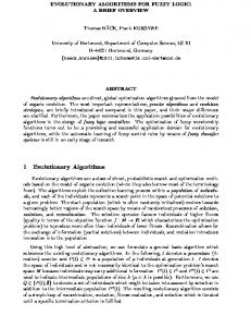
2-D shape matching experiments were conducted with a variety of target shapes, with all exhibiting similar performance. Results of one run are shown in Figures 1–3. The EA is quite effective since convergence of the test shape to the target shape occurs around the 60th iteration. Beyond this point, only small shape changes occur, due to decreasing self-adaptive, mutation rates. Results averaged over 25 runs for four different initial size ranges are shown in Table 2. The heading “Gens” indicates the number of iterations required for length convergence and “Fitness” is the fitness value of the final test shape. Several trends can be seen in these results. First, convergence to the correct size seems to be a valley-like function of initial range, with smaller ranges containing the target size converging more quickly. However, convergence to good fitness values seems to be dependent on having a larger range (or space) from which to search from initially. As in the proof of concept experiment, though, it seems that enlarging the range too much results in lower performance. Range 3–6 3–10 3–28 3–100

Gens. 5.09 2.79 4.08 5.91

σ 1.41 0.97 1.66 2.66

Fitness 209.71 192.99 110.04 175.41

σ 181.96 174.63 39.96 149.67

Table 2: Generations to length convergence and final fitness values for different initial ranges.

7 Iteration: 1

exG’s and its operators are generalizable to most other VLG’s. We show this by outlining how exG’s can be modified to mimic other VLG’s; in particular, those found in messy GA’s (mGA’s) and Virtual Virus (VIV). To conserve space, only the VLG’s are described in each case. The interested reader is referred to [1] and [4] for background on VIV and mGA’s respectively. 7.1

Figure 1: Target Shape and Best Shape for Iteration 1

Iteration: 15

Iteration: 25

GENERALITY OF exG’s

Messy GA’s

The messy coding used in mGA’s consists of strings of concatenated pairs of numbers. The first number is an integer ‘name’, while the second is a parameter value. The coding ((1 0)(3 1)), thus, denotes a genome with zero in the first bit and one in the third. The second bit is unspecified and is determined via a template. Bits can also be overspecified, as in ((3 1)(3 0)). In this case, the first occurrence is dominant; so, the third bit is zero. A new crossover operator is introduced that is a combination of two simpler operators called splice and cut. The splice operator simply concatenates two genomes into one, whereas a cut operator splits a single genome into two. Crossover is achieved by cutting two genomes, then splicing across the genomes. Mutation remains unchanged with bits randomly switching.

Figure 2: Best Shapes for Iterations 15 and 25

Iteration: 65

Iteration: 105

Messy coding can be achieved by exG’s if ranges of identifying gene values are associated with ‘names’. For example, say that an identifying gene in the range [1,2) corresponds to the first bit, [2,3) to the second, etc. We show how under and overspecification are handled in this exG with the examples used above. ((1 0)(3 1)) maps to something like ((1.1 0)(3.2 1)). Similarly, ((3 1)(3 0)) becomes something like ((3.1 1)(3.2 0)). Note that for exG’s, we must maintain order based on identifying genes. This fact precludes the use of the standard exG two point crossover, since a cut such as ((4 0)(2 1)(5 1)(3 1)(1 1)) to ((4 0)(2 1)) and ((5 1)(3 1)(1 1)) is not possible. The solution is to implement uniform crossover, where every gene has its own crossover probability. 7.2

Figure 3: Best shapes at iterations 65 and 105.

VIrtual Virus

Instead of binary or continuous valued strings, VIV uses a four valued alphabet in its genomes. In this case, the letters used are a, c, t, and g. Genomes are allowed to have different lengths, leading to a new crossover operator. Crossover occurs between homologous regions, or, in other words, blocks with the high-

est similarity are swapped during crossover. Crossover lengths are the same for both parents, but positions can vary. For example, the length 6 block starting from position 4 in P arent1 below will be swapped with the most similar length 6 block in P arent2 , which starts at position 2. Mutation, again, remains unchanged with genes randomly switching values. P arent1 : gggtttcgatttcatggtagcaaaaattag P arent2 : atttcgctcaggtaaatgcgcg VIV genomes can be mimicked by exG’s in the following manner. First, assign each letter a numerical value, say 1 for a, 2 for c, 3 for t, and 4 for g. Then, the identifying string is constructed by incrementing the previous gene value by the current letter’s value. For example, act would be (1 3 6). Mutation would then simply require updating the numerical values (e.g., mutation of act to aat results in (1 2 5)). Crossover implements a sliding/translating scheme. The P arent1 block is translated to the beginning of each valid P arent2 block to determine the closest match. For example, say the P arent1 block is (4 8 12), or ggg, and a length 3 block in P arent2 consists of (10 14 19), or agg. Then, the first block is translated so it starts from 10, leading to (10 14 18). If this is the most similar block, translation of the complete P arent1 genome by 6 allows standard 2 point exG crossover to be used in a equivalent fashion as VIV crossover in its coding scheme. 7.3

Notes on exG Generality

The previous discussions show that exG’s are able to replicate other VLG’s and their operators with slight modifications. This is not surprising, as most VLG’s have similar structures. In any event, it seems that imitating VLG’s with other VLG’s requires modifications to the coding scheme or operators, which may or may not be a trivial task.

8

CONCLUSION

A general variable length genome has been developed to address the problems of fixed dimensionality representations and application specific VLG’s. The newly developed VLG is shown to be an extension of canonical genomes; hence, the name extended genome, or exG. Experimental results of EA’s using exG’s are promising, as rapid convergence to optimal lengths is exhibited. The results also are in line with the theoretical discussions on SAGA and exG convergence. Furthermore, the utility of exG’s in real EA applications is shown in the 2-D shape matching experiments. Some

thoughts on how to modify exG’s into other VLG’s are also presented in an attempt to show the general applicability of exG’s.

References [1] Burke, D., DeJong, K., Grefenstette, J., Ramsey, C., and Wu, A. Putting more genetics into genetic algorithms. Evolutionary Computation 6, 4 (1998), 387–410. [2] Dasgupta, D., and Michalewicz, Z., Eds. Evolutionary Algorithms in Engineering Applications. Springer, Berlin, Germany, 1997. [3] Gen, M., and Cheng, R. Genetic Algorithms and Engineering Design. John Wiley, New York, 1997. [4] Goldberg, D., Deb, K., and Korb, B. Messy genetic algorithms: Motivation, analysis, and first results. Complex Systems 3 (1989), 493–530. [5] Goldberg, D. E. Genetic Algorithms in Search, Optimization, and Machine Learning. AddisonWesley Publishing Company, Inc., New York, 1989. [6] Harvey, I. The SAGA cross: The mechanics of crossover for variable-length genetic algorithms. In Parallel Problem Solving from Nature 2 (Cambridge, MA, 1992), Elsevier, pp. 269–278. [7] Harvey, I. Species Adaptation Genetic Algorithms: A basis for a continuing SAGA. In Proceedings of First European Conference on Artificial Life (Cambridge, MA, 1992), MIT Press, pp. 346–354. [8] Holland, J. H. Adaptation in natural and artificial systems. The University of Michigan Press, Ann Arbor, Michigan, 1975. [9] Kauffman, S., and Levin, S. Towards a general theory of adaptive walks on rugged landscapes. Journal of Theoretical Biology 128 (1987), 11–45. [10] Schwefel, H.-P. Evolution and Optimum Seeking. John Wiley, New York, 1995. [11] Winter, G., Periaux, J., Galan, M., and Cuesta, P., Eds. Genetic Algorithms in Engineering and Computer Science. John Wiley, New York, 1995.