Variable range of the RKKY interaction in edged graphene

arXiv:1308.6513v1 [cond-mat.mes-hall] 29 Aug 2013

Variable range of the RKKY interaction in edged graphene J. M. Duffy(a) , P. D. Gorman(a) , S. R. Power(c) and M. S. Ferreira(a,b) a) School of Physics, Trinity College Dublin, Dublin 2, Ireland b) CRANN, Trinity College Dublin, Dublin 2, Ireland c) Center for Nanostructured Graphene (CNG), DTU Nanotech, Department of Micro- and Nanotechnology, Technical University of Denmark, DK-2800 Kongens Lyngby, Denmark PACS numbers: Abstract. The indirect exchange interaction is one of the key factors in determining the overall alignment of magnetic impurities embedded in metallic host materials. In this work we examine the range of this interaction in magnetically-doped graphene systems in the presence of armchair edges using a combination of analytical and numerical Green function (GF) approaches. We consider both a semi-infinite sheet of graphene with a single armchair edge, and also quasi-one-dimensional armchair edged graphene nanoribbons (GNRs). While we find signals of the bulk decay rate in semi-infinite graphene and signals of the expected one-dimensional decay rate in GNRs, we also find an unusually rapid decay for certain instances in both, which manifests itself whenever the impurities are located at sites which are a multiple of three atoms from the edge. This decay behavior emerges from both the analytic and numerical calculations, and the result for semi-infinite graphene can be interpreted as an intermediate case between ribbon and bulk systems.

Variable range of the RKKY interaction in edged graphene

2

1. Introduction Graphene, the two-dimensional carbon allotrope, has been in the scientific limelight for almost a decade now due to a range of fascinating and experimentally realizable physical properties [1–5]. Interest in this material is further fueled by its potential application in a variety of fields, including spintronics, which attempts to exploit the charge and spin degrees of freedom of electrons in order to develop the next generation of nanoscale devices. Graphene is predicted to display very weak spin-orbit and hyperfine interactions which are common sources of spin-scattering and decoherence, and thus appears as a promising candidate material for the transport of spin information in such devices [6,7]. Fundamental to the field of spintronics is the indirect exchange coupling (IEC) which determines the alignment of magnetic objects in metallic systems. This interaction, mediated by the conduction electrons of the metallic host, makes separate magnetic objects aware of their mutual presence and forces the magnetizations to adopt the most energetically favorable alignment. When calculated in the framework of second order perturbation theory, the IEC is commonly known as the Ruderman-Kittel-KasuyaYosida (RKKY) interaction [8–12]. Despite their slight distinction, both terminologies are often used interchangeably and will be adopted here as equivalent. The investigation of the IEC in multilayer systems played a pivotal role in the development of the early spintronic devices, such as giant magnetoresistance stacks and spin valves [13–15]. Recently, experimental progress has been made in measuring the interaction between individual magnetic atoms on surfaces [16–18]. The basic features of the interaction are well documented, and it is generally seen to oscillate and decay as a function of the separation between the magnetic objects. The oscillation period is closely linked to the Fermi surface of the host material, and the decay rate to the dimensionality of the system. In a two dimensional host, the RKKY interaction between magnetic impurity atoms is predicted to decay with the square of the separation, D, between the impurities (D −2 ). The nature of such an interaction in a graphene system has been the subject of much discussion in recent literature [19–34]. The general consensus from these studies is that the interaction in graphene is shorter ranged due to the vanishing density of states at the Dirac point and decays as D −3 . Another curiosity is the oscillatory nature of the interaction, which is evident in most materials but hidden in graphene by a commensurability effect between the oscillation periods and the underlying hexagonal lattice. Furthermore, the interaction in graphene is predicted to have a sublattice dependence, i.e., magnetic moments on the same sublattice are predicted to align ferromagnetically, whereas those on opposite sublattices will pair antiferromagnetically. Despite the vast literature regarding the IEC in graphene, the body of work dedicated to edged graphene is surprisingly small [25, 27, 35–38]. This is particularly glaring in light of the fact that many of graphene’s local properties (e.g. transport, magnetic and mechanical) are drastically modified near the termination of the graphene lattice [19, 39–44]. Thus far, most of the attention has been focused on edges with

Variable range of the RKKY interaction in edged graphene

3

a zigzag geometry, where localized states were predicted to give rise to spin-polarized edges [19, 45–47]. Such magnetic-edged ribbons have inspired a number of theoretical device proposals [23,48–50]. Furthermore, success in the accurate patterning of graphene edges [51–53] makes this field more accessible from an experimental perspective, and attractive from a theoretical one. RKKY interactions mediated by the edge states in zigzag nanoribbons are expected to decay exponentially [25], in contrast to the powerlaw decay normally associated with the IEC in metallic systems. However, the presence of electron-electron interactions has been predicted to lead to a distance independent interaction [27]. Results in armchair nanoribbons are scarce, however, one study finds an interaction dependent on the distance from the edge [38] including both an exponential decay and a distance-independent interaction. To our knowledge, the IEC in graphene with a single edge has not been investigated previous to the current work. Motivated by the growing interest in the properties of edged graphene, we examine how the IEC between magnetic objects in graphene is affected by their proximity to an edge. Two situations are worth considering, namely the case of a single edge represented by a semi-infinite graphene sheet and the case of two parallel edges which is present in a graphene nanoribbon. In both these situations we will examine pristine armchair geometry edges, and focus on the range of the interaction between two localized magnetic moments with a separation DA parallel to the edge(s), as illustrated schematically in Figure 1. The interaction range is characterized by the rate of decay DA−α of the IEC and we show that α becomes a function of the distance from the edge in both cases. In other words, rather than displaying a fixed rate of decay as in bulk graphene, the IEC in edged graphene fluctuates between a long- and short-ranged interaction depending on how far the magnetic objects are from the armchair edges. Numerical calculations of the RKKY interaction are backed up by simple analytical expressions which are derived to explain the variations of the interaction range as the proximity to the graphene edges varies. Furthermore, we demonstrate that these variations are the result of interference effects introduced by the presence of one or more edges. In what follows we begin by presenting the model used to calculate the IEC and to describe the system under consideration. Special attention is paid to the single-particle Green functions (GFs) of the system, since they are the key ingredients appearing in the IEC expressions. We demonstrate alternative methods to calculate the GFs for a semiinfinite graphene sheet and examine how they relate to their infinite sheet counterparts. The GFs derived are very general quantities, and may be used to calculate a wide range of other physical properties in semi-infinite graphene and armchair nanoribbons. Results for both cases are presented, followed by a general discussion of the features observed in the numerical calculations and their connection with the analytical model. We finish with a section addressing our conclusions and an outlook on future work in edged graphene systems.

Variable range of the RKKY interaction in edged graphene

4

Figure 1. A schematic of our system. The dotted lines represent a continuation of the system and the dashed red line marks the x-axis (where DZ = 0) The dashed rectangle at the center is our two-atom unit cell, containing an atom from each of the two sublattices (• and ◦). The impurities are represented by larger, blue dots. The separation shown is given by DZ = 4, DA = 2 within our convention.

2. Model Let us start by defining the system to be studied, consisting of an armchair edged graphene sheet with two embedded magnetic objects, labeled A and B, both at a distance DZ (zigzag direction) from the edge. This setup is shown schematically in Figure 1. The magnetic objects are assumed to be substitutional magnetic impurities replacing two carbon atoms a distance DA apart in the armchair direction, although the results are equally valid for top-adsorbed impurities. Note that the distances DA and DZ cannot adopt any continuous values but are limited by the constrained integer values defining the hexagonal lattice. In other words, DZ is calculated in units of a2 (thus √ counting the number of atoms from the edge), and DA in units of 3a (thus counting the number of unit cells in the armchair direction), where a is the lattice parameter of graphene. Note that, under this definition, atoms at the very edge of the sheet take the value DZ = 1. The IEC between the two magnetic impurities A and B can be calculated as the total energy difference between their ferromagnetic and antiferromagnetic configurations. Using the Lloyd formula method [54, 55] this energy difference is given by Z ∞ 1 dE f (E) ln(1 + 4Vx2 G↑BA (E)G↓AB (E)), (1) JBA = − Im π −∞

where Vx is the exchange splitting between the spin sub-bands of the magnetic impurities, f (E) the Fermi function and GσBA (E) is the single-particle GF between the impurities A and B for electrons with spin σ with the system in the ferromagnetic

Variable range of the RKKY interaction in edged graphene

5

configuration. The spin dependent GFs Gσ can be calculated in terms of their pristine lattice counterparts g by introducing a localized potential term describing the bandsplitting at the magnetic impurity sites using Dyson’s equation. Within this convention a negative coupling represents favorable ferromagnetic alignment, and a positive coupling an antiferromagnetic one. If the coupling is expanded to lowest order in Vx , we can recover the standard perturbative form of the RKKY interaction, also given by the spin susceptibility of the system Z ∞ 4Vx2 2 Im dE f (E)gBA (E), (2) JRKKY = − π −∞

where g is now the GF of the pristine system in the absence of any magnetic impurities. To proceed it is important to specify the Hamiltonian defining the electronic structure of graphene, which in this case is described by the nearest-neighbour tightbinding approximation representing the electrons in the pz orbitals of the carbon atoms: XX |r, αithr′, β| . (3) H= r,r′ α,β

Graphene is formed from two interlocking triangular sublattices, and our notation is chosen accordingly. |r, αi labels a π orbital at the site whose unit cell is given by r and whose sublattice is defined by the index α = • or α = ◦ (see Figure 1). We note from Eqs. (1) and (2) that the separation dependence of the interaction is entirely within the GFs. Thus the distance dependent features of this interaction can be described entirely by examining these quantities, which are derived in the next section. 2.1. Single-particle Green Functions First we derive the GF for bulk graphene and then show how this approach may be expanded to deal with semi-infinite graphene. The GF associated with a Hamiltonian H is given by  −1 ˆ ˆ gˆ(E) = E I − H . (4)

The Hamiltonian for bulk graphene given in Eq. (3) can be greatly simplified by Fourier transforming to reciprocal space (|k, αi), and it may be completely diagonalized by the following choice of eigenstates   f † (k) 1 |k, ◦i , (5) |k, ±i = √ |k, •i ± |f (k)| 2   √ 3 where f (k) = 1 + 2eikx 2 a cos ky2a . Diagonalization makes the inversion in Eq. (4) trivial and the GF may now be written as X |k, +ihk, +| |k, −ihk, −| gˆ(E) = + . (6) E − t|f (k)| E + t|f (k)| k

Variable range of the RKKY interaction in edged graphene This can be projected onto the position basis to get √ Z Z N αβ (E, k)eik·(r2 −r1 ) a2 3 dk dk , hr1 , α|ˆ g(E)|r2 , βi = y x 8π 2 E 2 − t2 |f (k)|2

6

(7)

where the integration is taken over the first Brillouin Zone in reciprocal space. Here N αβ (E, k) is a sublattice dependent term given by   α=β  E αβ N (E, k) = (8) tf (k) α = •; β = ◦   tf † (k) α = ◦; β = • .

In order to calculate the GF for semi-infinite graphene it is necessary to first obtain a suitable basis of eigenstates. We consider the following linear combination of bulk states 1 |φk , ±i = √ (|(kx , ky ), ±i − |(kx , −ky ), ±i) , (9) 2 where the vector k is written explicitly in terms of its components kx and ky , and we examine its projection on the position basis i h(x, y), •|φk, ±i = − √ e−ikx x sin(ky y) N i f † (k) h(x, y), ◦|φk, ±i = ∓ √ e−ikx x sin(ky y) . |f (k)| N It is clear that the projection vanishes whenever y = 0, indicating that there are no longer any atomic states along the x-axis. This means that the graphene sheet has been divided up into two equivalent halves, the layout of which can be seen in Fig. 2. With the new choice of eigenstates the semi-infinite GF is given by X |φk , +ihφk , +| |φk , −ihφk , −| ˆ + , (10) S(E) = E − ǫ+ E + ǫ+ and this can be similarly projected onto the position basis to get √ Z Z a2 3 dky dkx h(x1 , y1 ), α|S(E)|(x2 , y2 ), βi = 4π 2 N αβ (E, k)eikx (x2 −x1 ) sin(ky y1 ) sin(ky y2 ) . (11) × E 2 − t2 |f (k)|2

One of these integrals can be solved by contour integration, upon which the GF between two atoms a distance DZ from the edge and separated by a distance DA in the armchair direction is given by Z π 2 E e2iqDA sin2 (kZ DZ ) i dk S(E, DZ , DA ) = , (12) Z 2πt2 − π2 cos(kZ ) sin(q) where q is the pole from the contour integration and is given by   2 2 2 2 −1 E − t − 4t cos (kZ ) , q = ± cos 4t2 cos(kZ )

(13)

and the sign of the pole is chosen such that its imaginary √part is always positive. Here we have introduced the dimensionless k-space vectors kA = 23a kx and kZ = a2 ky . Numerical

Variable range of the RKKY interaction in edged graphene

7

integration gives the GF exactly, but we can also use the stationary phase approximation (SPA) to find an approximate analytic form of the GF, and we do so later in this paper. The fact that we have formed the semi-infinite GF by considering combinations of bulk eigenstates makes it natural to see whether the semi-infinite GF can be written in terms of its bulk counterparts. It turns out that this is both possible to do, and provides geometric insight into its meaning. 2.2. The Image Method As previously mentioned, the IEC in bulk graphene has been extensively studied and most of its features are well understood. Therefore, our strategy is to express the semi-infinite system representing a single-edged graphene sheet in terms of its bulk counterpart so that we can infer the IEC behavior in the presence of edges. Such a strategy requires that we relate the semi-infinite GF to that of bulk graphene. In order to express the semi-infinite GF in terms of the more familiar bulk GFs we expand out the eigenstates in Eq. (10) in terms of their bulk equivalents of Eq. (9). Collecting all the positive ky terms (|(kx , ky ), ±i) leads to the general formula for the bulk GF (Eq. 6). The problem that arises is in dealing with terms that have a −ky , such as X |(kx , ky ), +ih(kx, −ky ), +| |(kx , ky ), −ih(kx , −ky ), −| + . (14) gˆ2 (E) = E − ǫ+ E + ǫ+ These quantities can be dealt with by noting that, when dealing with the projection of a reciprocal-space state onto the real space, the minus sign can be freely swapped between ky and y. By means of a Fourier transform, it can be shown that h(x, y), α|(kx, −ky ), ±i = h(x, −y)|(kx, ky ), ±i.

(15)

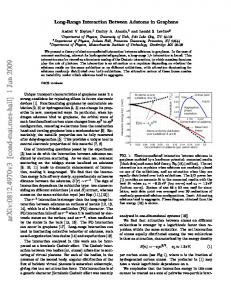
Thus a sign change in ky is equivalent to a reflection of the position vector about the y-axis. Now hr1 , α|g2(E)|r2 , βi can be seen as the GF between r1 and the reflection of r2 . This method can be applied to the remaining factors, allowing us to write the semi-infinite GF between A and B as 1 SAB (E) = (gAB (E) − gAB′ (E) − gA′ B (E) + gA′ B′ (E)) 2 (16) = gAB (E) − gAB′ (E) , where A′ and B ′ are the images of A and B as shown in Fig. 2, which also underlines the simplicity and intuitive nature of the approach. From Eq. 16 and Fig. 2 we see that the Green function connecting two sites on the semi-infinite lattice is equivalent to that on the infinite lattice with the addition of a correction term that takes into account the edge-induced scattering. This correction term is simply the Green function connecting one site with the site equivalent to the image of the other in the infinite graphene sheet with a phase shift of π. This rather intuitive and computationally convenient result is a direct consequence of the simple manner in which the bands of armchair-edged graphene can be written in terms of their infinite sheet counterparts. For other edge geometries, the presence of localized edge states which cannot easily be reconciled with

Variable range of the RKKY interaction in edged graphene

8

Figure 2. A semi-infinite Green function between A and B can be written as a sum of bulk terms between A, B and their image sites A′ , B ′

the infinite graphene band structure complicate the picture and prevent the formulation of the simple relation given in Eq. 16. Furthermore the entire DZ dependence of the semi-infinite sheet GF is contained within this correction term, and from the standard behavior of the graphene GF we can determine that it will decay with increased distance 1 . Thus, when dealing with atoms a long distance from the edge, from the edge as √D Z ′ we will find that gAB (E)