Variable stepsize Runge-Kutta methods for stochastic wave equations

arXiv:quant-ph/0406092v1 14 Jun 2004

Variable stepsize Runge-Kutta methods for stochastic wave equations Joshua Wilkie and Murat C ¸ etinba¸s Department of Chemistry, Simon Fraser University, Burnaby, British Columbia V5A 1S6, Canada Abstract. We show that existing Runge-Kutta methods for ordinary differential equations (odes) can be modified to solve stochastic differential equations (sdes) with strong solutions provided that appropriate changes are made to the way stepsizes are selected. The order of the resulting sde scheme is half the order of the ode scheme. Specifically, we show that an explicit 9th order Runge-Kutta method (with an embedded 8th order method) for odes yields an order 4.5 method for sdes which can be implemented with variable stepsizes. This method is tested by solving systems of sdes originating from stochastic wave equations arising from master equations and the many-body Schr¨ odinger equation.

PACS numbers: 03.65.-w, 02.50.-r, 02.70.-c

Variable stepsize Runge-Kutta methods for stochastic wave equations

2

1. Introduction Stochastic wave equations play an important role in the quantum theory of decoherence and measurement[1, 2] as well as in computational many-body physics[3, 4, 5, 6]. Solutions of master equations for completely positive dynamical semigroups[3] and for Redfield theory[2] can be expressed as expectations of diadics formed from wavefunctions obeying stochastic wave equations. Recently it has been shown that exact solutions of the N-body Schr¨odinger or Liouville-von Neumann equations can be expressed as averages of Hartree products of single-body wavefunctions or densities which obey stochastic wave equations[3, 4, 5, 6]. Such methods could have important applications in chemistry and condensed matter physics. Stochastic differential equations (sdes) are also widely employed in other areas of physics, engineering and finance[7]. Unfortunately, efficient numerical techniques for solving such equations have not yet been developed. Algorithms in the literature have not substantially improved on the primitive methods described ten years ago in the well known text by Kloeden and Platen[8]. Methods applicable to general systems of stochastic differential equations with multiple Wiener processes have not exceeded an order of 2. The low order of such methods restricts their domain of usefulness to one or few equations, and the larger systems of equations of interest in physics cannot be solved. Recently, one of us noted[9] that with minor modifications classical methods for ordinary differential equations (odes) can be used to solve sdes with strong solutions. The technique was demonstrated by solving a wide range of low dimensional sdes with known exact solutions[9]. Here we expand upon this idea by developing variable stepsize (i.e. adaptive) explicit Runge-Kutta based integrators for sdes. We demonstrate the use of the method by solving a variety of stochastic wave equations arising in decoherence problems[1], and in stochastic decomposition of the many-body problem[3, 4, 5, 6]. 2. Stochastic Taylor expansion There is a close connection between Taylor expansions of solutions of odes and Taylor expansions of strong solutions of sdes[9]. Consider a finite set of sdes, dXtj

j

= a (Xt , t) dt +

m X

bjk (Xt , t) dWtk ,

(1)

k=1

represented in Itˆ o[8] form, where j = 1, . . . , n. Here Xt = (Xt1 , . . . , Xtn ) and the dWtk are independent and normally distributed stochastic differentials with zero mean and variance dt (i.e. sampled N (0, dt)). The stochastic variables Wtk are Wiener processes. Assume that the coefficients aj and bjk have regularity properties which guarantee strong solutions, i.e. that Xtj are some fixed functions of the Wiener processes, and that they are differentiable to high order. We may then view the solutions of (1) as functions Xtj = Xj (t, Wt1 , . . . , Wtm ) of time and the Wiener processes. The solutions can therefore be expanded in Taylor series. Keeping terms of order dt or less then gives m X ∂Xtj ∂Xtj j dWtk dt + Xt+dt = Xtj + k ∂t ∂W t k=1

Variable stepsize Runge-Kutta methods for stochastic wave equations +

1 2

m X

∂ 2 Xtj dWtk dWtl . k ∂W l ∂W t t k,l=1

3 (2)

The product of differentials dWtk dWtl is equivalent to δk,l dt in the Itˆ o[8] formulation of stochastic calculus, so that m 1 X ∂ 2 Xtj ∂Xtj j j ] dt + dXt+dt = Xt+dt − Xtj = [ ∂t 2 ∂Wtk2 k=1 +

m X ∂Xtj dWtk . k ∂W t k=1

(3)

Comparison to (1) allows us to identify the first derivatives ∂Xtj = bjk (Xt , t) ∂Wtk

(4) m

1 X ∂ 2 Xtj ∂Xtj = aj (Xt , t) − ∂t 2 ∂Wtk2 = aj (Xt , t) −

1 2

k=1 m X n X

bik (Xt , t)

k=1 i=1

∂bjk (Xt , t) . ∂Xti

(5)

From these first order derivatives, expressed in terms of aj and bjk , higher order derivatives can be computed. Thus a Taylor expansion of the solutions m X ∂Xtj ∂Xtj j ∆t + ∆Wtk Xt+∆t = Xtj + k ∂t ∂W t k=1 +

m 1 X ∂ 2 Xtj ∆Wtk ∆Wtl + . . . k ∂W l 2 ∂W t t k,l=1

(6)

can be obtained for finite displacements ∆t and ∆Wtk . 3. Runge-Kutta methods for sdes This Taylor expansion of strong solutions of sdes can be employed to develop RungeKutta algorithms and other integration schemes[9]. As an example consider the classic fourth order Runge-Kutta scheme with four stages Kj1

= fj (Xti , ti ) 1 1 Kj2 = fj (Xti + K1 , ti + ∆t) 2 2 1 1 Kj3 = fj (Xti + K2 , ti + ∆t) 2 2 Kj4 = fj (Xti + K3 , ti+1 ) 1 Xti+1 = Xti + (K1 + 2K2 + 2K3 + K4 ) 6 with fj (Xt , t) defined via m

fj (Xt , t) =

X ∂X j ∂Xtj t ∆t + ∆Wtk ∂t ∂Wtk k=1

(7)

Variable stepsize Runge-Kutta methods for stochastic wave equations = [aj (Xt , t) − +

m X

1 2

n m X X k=1 i=1

bjk (Xt , t)∆Wtk .

bik (Xt , t)

4

∂bjk (Xt , t) ]∆t ∂Xti (8)

k=1

Here ti is the initial time and ti+1 = ti +∆t. Taylor expansion shows that Xti+1 differs from the exact solution by terms of order higher than ∆t2 (i.e. terms of higher order than ∆t2 , ∆t(∆Wtk )2 , (∆Wtk )4 , (∆Wtk )2 (∆Wtl )2 , and (∆Wtk )2 ∆Wtl ∆Wti ). Thus, this stochastic Runge-Kutta algorithm is very similar to its classical counterpart except that its order is 2 not 4. Generalizations to higher order Runge-Kutta schemes are straightforward. One simply replaces the usual stage evaluations of Runge-Kutta with evaluations of (8). Since (8) is order ∆t1/2 rather than order ∆t, the order of the sde method is half that of the ode method. SDE methods of order 2 and 4 constructed in this fashion have been shown to be very accurate in fixed stepsize calculations for small systems of sdes[9]. In this manuscript we adapt a 9th order Runge-Kutta method[14] with 16 stages into an order 4.5 method for sdes. However, fixed stepsize Runge-Kutta methods are neither accurate nor efficient for general systems of equations. To solve the large systems of sdes that arise in physical problems we need some means of controlling the local error. 4. Adaptive stepsizes Local error is typically controlled in Runge-Kutta schemes for odes via the use of embedded lower order methods[10, 11, 12, 13]. That is, Runge-Kutta methods can often be found wherein a method of order l with k ≥ l stages has an embedded RungeKutta scheme of order l − 1 which uses some subset of the k stages of the higher order method. Differences in the two solutions can be compared to a user requested tolerance to decide whether a contemplated step can be accepted or whether a smaller stepsize should be considered. Thus local error can be estimated, and stepsizes adapted to ensure the accuracy of the solution, at negligible extra cost. Well implemented examples of this approach are the 5(4) and 8(7) embedded pairs of Dormand and Prince (see [12] and [13], respectively) which form the basis of the ode software package RKSUITE. A 9(8) pair has been derived by Tsitouras[14] although this algorithm has not been included in any software of which we are aware. Runge-Kutta methods of order 10 are known[15] but embedded lower order pairs have not been reported. Variable stepsize one step schemes such as Runge-Kutta are popular because they are simple to understand and easy to implement. Multi-step schemes, such as Predictor-Corrector[16], which store and use information from previous steps are however often much faster and more accurate. Unfortunately, it is not clear how the stochastic Taylor expansion developed above can be incorporated into a multi-step scheme. Predictor-Corrector[16], for example, employs Lagrange type interpolation formulae (to fit fj (Xt , t) at a set of times), which are explicitly integrated over a time interval, to construct both the predictor and the corrector. It is far from clear how an analogous scheme would work for the m + 1 variables t, W1 , . . . , Wm . Thus, Runge-Kutta methods seem to be the easiest to develop for sdes. Once an error has been judged too large to be acceptable, ode codes simply try a smaller step and all information about the original step is lost. This procedure

Variable stepsize Runge-Kutta methods for stochastic wave equations

5

obviously cannot yield unbaised solutions in an analogous scheme for sdes. Therefore measures must be taken to ensure that the original Wiener process is maintained. One way of doing this is to halve the original step and to generate stochastic differentials on the two subintervals such that their sum is the original step. This approach was originally proposed by Gaines and Lyons[17] and is known as the method of binary Brownian trees. More sophisticated strategies have since been developed[18] but they are specific to individual algorithms and cannot be easily adapted for our purposes. A number of schemes have been proposed for choosing the stochastic differentials on the subintervals[17, 19]. The correct approach appears to be that of Lamba[19] who generates the stochastic differential on the first subinterval by sampling the conditional probability R∞ dxa dxb p(xa )p(xb )δ(∆Wa − xa )δ(xa + xb − ∆W ) p(∆Wa ; ∆W ) = −∞ R ∞ dxa dxb p(xa )p(xb )δ(xa + xb − ∆W ) −∞

(∆Wa − ∆W/2)2 1 } (9) exp{− = p 2(∆t/4) 2π(∆t/4) where ∆W is the original stochastic differential, ∆Wa is the stochastic differential on the first subinterval and 1 x2 p(x) = p } (10) exp{− 2(∆t/2) 2(∆t/2)

is the independent density for differentials on the subintervals. This implies that the stochastic differential ∆Wa on the first subinterval has mean ∆W/2 and variance ∆t/4. The stochastic differential on the second subinterval ∆Wb must then be given by ∆Wb = ∆W − ∆Wa in order to maintain the original Wiener process. Thus, Runge-Kutta methods can be developed for sdes with strong solutions from Runge-Kutta methods for odes, and a binary tree variable stepsize strategy can be implemented with sampling on the subintervals via Lamba’s method[19]. To show that the combined approach yields an accurate numerical method we solve a variety of stochastic wave equations from the recent physics literature. With the adaptive stepsize strategy we have chosen there is a good correlation between the speed of an algorithm and its order. We thus chose to employ the highest order Runge-Kutta pair available, which as far as we are aware is the 9(8) pair of Tsitouras[14]. We have sucessfully used other lower order methods such as those of [12] and [13], but for consistency all results reported in this paper were calculated using the method described in [14]. 5. Examples Here we solve 3 sets of equations from the recent physics literature using the order 4.5 Runge-Kutta method implemented with variable stepsizes as described above. 5.1. The first example we consider is the Gisin-Percival[1] stochastic wave equation for the nonlinear absorber (Eq. 4.2 of Ref. [1]) d|Ψ(t, Wt )i = .1(a† − a)|Ψ(t, Wt )idt + (2ha†2 ia2 − a†2 a2 − |ha2 i|2 )|Ψ(t, Wt )idt √ + 2(a2 − ha2 i)|Ψ(t, Wt )idWt

(11)

6

Variable stepsize Runge-Kutta methods for stochastic wave equations

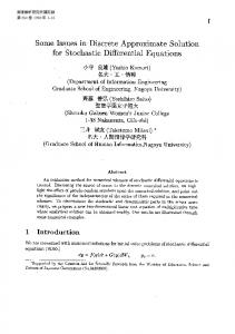
where a denotes the usual harmonic oscillator lowering operator. We chose an initial state |Ψ(0, 0)i = |0i where |0i is the lowest eigenstate of a† a. We choose W0 = 0 in this and later examples and the Wiener process Wt is real. The notation hY i indicates the quantum expectation hΨ|Y |Ψi. The ensemble average over statistical realisations of the Wiener processes is denoted via M [Y ] for any Y . The quantity of interest for this example is the average density ρ(t) = M [|Ψ(t, Wt )ihΨ(t, Wt )|]

(12)

which obeys the deterministic master equation dρ(t) = .1[a† − a, ρ(t)] + 2a2 ρ(t)a†2 − a†2 a2 ρ(t) − ρ(t)a†2 a2 . dt

(13)

1 0.9 0.8 0.7 0.6 0.5 0.4 0.3 0.2 0.1 0 0

50

100

150 t

200

250

300

Figure 1. Mean occupation number nt vs. time t

To implement our approach we need to find the derivatives of |Ψ(t, Wt )i with respect to t and Wt . We immediately see that ∂|Ψ(t, Wt )i √ 2 = 2(a − ha2 i)|Ψ(t, Wt )i (14) ∂Wt and using (5) we also determine that ∂|Ψ(t, Wt )i = .1(a† − a)|Ψ(t, Wt )i + (ha4 i − ha2 i2 )|Ψ(t, Wt )i ∂t − (a2 − ha2 i)2 |Ψ(t, Wt )i + (ha†2 a2 i − |ha2 i|2 )|Ψ(t, Wt )i + (2ha†2 ia2 − a†2 a2 − |ha2 i|2 )|Ψ(t, Wt )i. (15)

From these results we can now construct fj (Xt , t) using Eq. (8). The Runge-Kutta scheme can thus be implemented as discussed above. The dynamics was solved in a basis consisting of the lowest 11 eigenstates |ni of a† a with n = 0, . . . , 10. Thus, including real and imaginary parts of hn|Ψ(t, Wt )i for n = 0, . . . , 10 our equations

Variable stepsize Runge-Kutta methods for stochastic wave equations

7

consist of a total of 22 real nonlinear coupled stochastic equations. A relative tolerance of 10−13 was requested. In Fig. 1 we plot the mean occupation number nt = Tr{a† aρ(t)} vs time for 50000 stochastic realisations (dashed curve) and for an exact solution of Eq. (13) performed in the same basis set (solid curve). Agreement is very good. Due to the increasing number of Wiener processes in the following examples, we drop the Wt ’s as arguments of the stochastic wavefunctions. This change of notation is necessary but regretable since this dependence is an essential requirement of the method we are testing. 5.2. The second example is the Gisin-Percival[1] stochastic wave equation for a quantum cascade with absorption and stimulated emission (Eq. 4.4 of Ref. [1]) d|Ψ(t)i = − .1i(a† + a)|Ψ(t)idt

+ (2ha† ai a† a − (a† a)2 − (ha† ai)2 )|Ψ(t)idt + .01(2ha† ia − a† a − |hai|2 )|Ψ(t)idt √ + 2(a† a − ha† ai)|Ψ(t)idWt1 √ + .1 2(a − hai)|Ψ(t)idWt2 .

(16)

Here again we chose the initial state |Ψ(0)i = |0i. There are now 2 real statistically independent Wiener processes (i.e. M [dWt1 dWt2 ] = 0). The quantity of interest is again the density (12) which in this case obeys the master equation dρ(t) = − .1i[a† + a, ρ(t)] + 2a† aρ(t)a† a − (a† a)2 ρ(t) − ρ(t)(a† a)2 dt + .02aρ(t)a† − .01a† aρ(t) − .01ρ(t)a† a. (17)

The derivatives of |Ψ(t)i with respect to t, Wt1 and Wt2 are given by ∂|Ψ(t)i √ † = 2(a a − ha† ai)|Ψ(t)i ∂Wt1 √ ∂|Ψ(t)i = .1 2(a − hai)|Ψ(t)i 2 ∂Wt ∂|Ψ(t)i = −.1i(a† + a)|Ψ(t)i ∂t + (2ha† ai a† a − (a† a)2 − (ha† ai)2 )|Ψ(t)i

(18) (19)

+ .01(2ha† ia − a† a − |hai|2 )|Ψ(t)i − (a† a − ha† ai)2 |Ψ(t)i + 2(h(a† a)2 i − ha† ai2 )|Ψ(t)i

− .01(a − hai)2 |Ψ(t)i + .01(ha† a)i − |hai|2 )|Ψ(t)i + .01(ha2 i − hai2 )|Ψ(t)i.

(20)

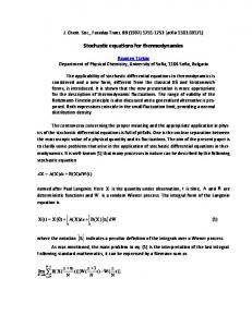
The same basis set and tolerance as in example 1 were employed. Again we calculated the mean occupation number for 50000 trajectories (dashed curve) and for an exact solution of Eq. (17) (solid curve). These quantities are plotted in Fig. (2). Agreement is again good but convergence is somewhat slower than in example 1 since we now have twice as many Wiener processes.

8

Variable stepsize Runge-Kutta methods for stochastic wave equations 1 0.9 0.8 0.7 0.6 0.5 0.4 0.3 0.2 0.1 0 0

50

100

150 t

200

250

300

Figure 2. Mean occupation number nt vs. time t

5.3. The third example consists of stochastic wave equations for a stochastic decomposition of the Schr¨odinger equation for Helium[6]. Neglecting nuclear motion about the center of mass, the Helium wavefunction Φ(r1 , r2 , t) obeys the deterministic Schr¨odinger equation (in atomic units h ¯ = 1, me = 1, and e = 1) ∂Φ(r1 , r2 , t) = − iH2 Φ(r1 , r2 , t) (21) ∂t 2 1 1 1 2 − + = − i{− ∇21 − ∇22 − }Φ(r1 , r2 , t), 2 2 r1 r2 |r1 − r2 |

for any specified anti-symmetric initial state Φ(r1 , r2 , 0). Here r1 and r2 denote positions of electrons 1 and 2 with respect to the nucleus. For our example calculation we choose an initial wavefunction of the form Φ(r1 , r2 , 0) = β (Ψ1 (r1 , 0)Ψ2 (r2 , 0) − Ψ2 (r1 , 0)Ψ1 (r2 , 0)) p (where β = 1/ 2(1 − |hΨ1 (0)|Ψ2 (0)i|2 ) is a normalization factor) which is obviously antisymmetric in r1 and r2 . Note that we are implicitly incorporating the twocomponent electron spins into the definitions of Ψ1 and Ψ2 . For our purposes it is important that hΨ1 (0)|Ψ2 (0)i = 6 0. The actual initial conditions for this example calculation were chosen randomly as a mixture of 1s and 2s He+ states for each electron. It can be shown[6] that the exact deterministic wavefunction Φ(r1 , r2 , t) evolving from (5.3) can be decomposed into stochastic waves via an average of the form Φ(r1 , r2 , t) = βM [Ψ1 (r1 , t)Ψ2 (r2 , t) − Ψ2 (r1 , t)Ψ1 (r2 , t)]

(22)

Variable stepsize Runge-Kutta methods for stochastic wave equations

9

where Ψ1 and Ψ2 satisfy stochastic wave equations p X 1 2 dΨ1 (r, t) = [−i(− ∇2 − )Ψ1 (r, t) − i ωs hOs i2 Os Ψ1 (r, t) 2 r s=1 p

+

iX ωs hOs i1 hOs i2 Ψ1 (r, t)]dt 2 s=1

p X √ −iωs (Os − hOs i1 ) Ψ1 (r, t)dWts +

−

s=1 p X s=1

|ωs |

(23)

hΨ1 |Ψ1 i[hOs† Os i1 − |hOs i1 |2 ] Ψ2 (r, t)dt 2Re {hΨ1 |Ψ2 i}

p X 2 1 ωs hOs i1 Os Ψ2 (r, t) dΨ2 (r, t) = [−i(− ∇2 − )Ψ2 (r, t) − i 2 r s=1 p

+

iX ωs hOs i2 hOs i1 Ψ2 (r, t)]dt 2 s=1

+

p X √ −iω (Os − hOs i2 ) Ψ2 (r, t)dWts

−

s=1 p X s=1

|ωs |

(24)

hΨ2 |Ψ2 i[hOs† Os i2 − |hOs i2 |2 ] Ψ1 (r, t)dt. 2Re {hΨ1 |Ψ2 i}

We have used a notation hF ij = hΨj |F |Ψj i in the above equations. Here the ωs and operators Os arise through the one-body expansion of the Coulomb interaction p X 1 ωs Os (1)Os (2) (25) = |r1 − r2 | s=1 which we performed numerically in a basis of He+ eigenstates[6]. In the calculation reported here p = 8 which means that there are eight real Wiener processes. Since the initial states are of s type we included only the basis functions of s type with a principle He+ quantum number of 4 or less[6]. This means that the total number of equations was 32. Clearly this is by far the most computationally difficult of the three examples. The derivatives of Ψj (r, t) are given by ∂Ψj (r, t) √ = −iω (Os − hOs ij ) Ψj (r, t) ∂Wts p X 1 2 ∂Ψj (r, t) ωs hOs ik Os Ψj (r, t) = −i(− ∇2 − )Ψj (r, t) − i ∂t 2 r s=1 p

+

iX ωs hOs i1 hOs i2 Ψj (r, t) 2 s=1

−

p X

+

i 2

|ωs |

s=1 p X s=1

hΨj |Ψj i[hOs† Os ij − |hOs ij |2 ] Ψk (r, t) 2Re {hΨ1 |Ψ2 i}

ωs (Os2 − 2hOs ij Os + 2hOs i2j − hOs2 ij )Ψj (r, t)

10

Variable stepsize Runge-Kutta methods for stochastic wave equations +

1 2

p X s=1

|ωs |(hOs† Os ij − |hOs ij |2 )Ψj (r, t)

(26)

where k 6= j and j, k = 1, 2. From these equations we can now construct fj (Xt , t) using Eq. (8). 1 0.8 0.6 0.4 0.2 0 -0.2 -0.4 -0.6 -0.8 -1 0

5

10

15

20 t

25

30

35

40

20 t

25

30

35

40

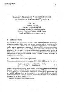
Figure 3. Re hΨ(0)|Ψ(t)i vs. t

1

0.8

0.6

0.4

0.2

0

-0.2

-0.4

-0.6

-0.8 0

5

10

15

Figure 4. Im hΨ(0)|Ψ(t)i vs. t

11

Variable stepsize Runge-Kutta methods for stochastic wave equations

A numerical problem arises in Eqs. (25) when the overlap hΨ1 |Ψ2 i becomes small. The terms inversely proportional to this factor vary rapidly and the speed of integration slows down greatly. This occurs every few atomic units. Fortunately, this can be easily avoided by adding a small piece of Ψ2 (r, t) to Ψ1 (r, t), renormalizing the wavefunctions, and carrying the new norm as a weight factor in the stochastic average. The antisymmetric nature of the full wavefunction guarantees that this manipulation makes no change in the solution. In Figs. (3) and (4) we plot the real and imaginary parts of hΦ(0)|Φ(t)i for 200000 trajectories (dashed curve) and for the exact solution (solid curve) of the Shr¨odinger equation (21). Agreement is satisfactory with some deterioration of accuracy as time proceeds. 4

3

2

1

0

-1

-2 -6

-4

-2

0 E

2

4

6

Figure 5. He energy spectrum

Finally, we computed the energy spectrum via   Z T iEt 1 dt ≃ hΨ(0)|δ(E−H2 )|Ψ(0)i(27) Re hΨ(0)|Ψ(t)i exp I(E) = π¯ h ¯h 0 which we plot in Fig. (5). Again satisfactory agreement is obtained. The fact that complete convergence is not achieved even with 200000 realisations may be due to the relatively large number of Wiener processes. Unfortunately, examples with very large numbers of Wiener processes will arise when the method of stochastic wave equations described in [6] is applied to larger atoms or molecules. Thus it may be necessary to explore some form of importance sampling to improve convergence for these simulation methods. 6. Discussion The numerical strategy discussed in this manuscript provides a method for solving the large sets of coupled nonlinear sdes which arise in physical problems. This is currently

Variable stepsize Runge-Kutta methods for stochastic wave equations

12

the best strategy for solving systems of sdes like those that arise from stochastic wave equations. However, the large number of stages (16 for [14]) required for high order Runge-Kutta formulae limit the efficiency of our approach. Multistep methods for odes such as Predictor-Corrector[16] typically require only two evaluations of derivatives per step and can be implemented to any desired order. If such methods could be adapted for sdes the gain in efficiency could be enormous. Unfortunately, to implement such a strategy would require interpolation in m + 1 variables with variable stepsizes (here m is the number of Wiener processes). At present we do not see how this can be accomplished. Acknowledgments The authors acknowledge the support of the Natural Sciences and Engineering Research Council of Canada. [1] N. Gisin and I. C. Percival, J. Phys. A 25, 5677 (1992). [2] P. Gaspard and M. Nagaoka, J. Chem. Phys. 111, 5676 (1999). [3] I. Carusotto and Y. Castin, Laser Physics 13, 509 (2003); I. Carusotto, Y. Castin, and J. Dalibard, Phys. Rev. A 63, 023606 (2001). [4] O. Juillet, Ph. Chomaz, Phys. Rev. Lett. 88, 142503 (2002). [5] J. Wilkie, Phys. Rev. E 67, 017102 (2003). [6] L. Tessieri, J. Wilkie and M. C ¸ etinba¸s, submitted for publication. [7] C.W. Gardiner, Handbook of stochastic methods, (Springer, Berlin, 1983). [8] P.E. Kloeden and E. Platen, Numerical solution of stochastic differential equations, (Springer, Berlin, 1995). [9] J. Wilkie, Phys. Rev. E, accepted for publication (2004). [10] W.H. Press, S.A. Teukolsky, W.T. Vetterling and B.P. Flannery, Numerical recipes, (Cambridge University Press, Cambridge, 1992). [11] E. Hairer, S.P. Norsett, G. Wanner, Solving ordinary differential equations, (Springer-Verlag, Berlin, 1993). [12] J.R. Dormand and P.J. Prince, J. Comput. Appl. Math. 6, 19 (1980). [13] P.J. Prince and J.R. Dormand, J. Comput. Appl. Math 7, 67 (1980). [14] Ch. Tsitouras, Appl. Num. Math. 38, 123 (2001). [15] E. Hairer, J. Inst. Maths. Applics. 21, 47 (1978). [16] L. F. Shampine and M. K. Gordon, Computer solution of ordinary differential equations : the initial value problem, (San Francisco, W.H. Freeman, 1975). [17] J.G. Gaines and T.J. Lyons, SIAM J. Appl. Math. 57, 1455 (1997). [18] See J. Leyn, A. R¨ obler and O. Schein, J. Comput. Appl. Math. 138, 297 (2002) and references therein. [19] H. Lamba, J. Comput. Appl. Math. 161, 417 (2003).