2(X, Y ) along y direction. Higher order schemes such as that ..... composed of the river,the lake and two islands as well as outflows. 2000 particles were initially ...
Water Pollution VIII: Modelling, Monitoring and Management
465
Variable time stepping in parallel particle models for transport problems in shallow waters W. M. Charles1 , E. van den Berg2 , H. X. Lin1 & A. W. Heemink1 1 Delft
University of Technology, Faculty of Electrical Engineering, Mathematics and Computer Science, Department of Applied Mathematical Analysis, Delft, The Netherlands 2 University of British Columbia, Canada
Abstract Stochastic differential equations (SDEs) are stochastic in nature. The SDEs under consideration are often called particle models (PMs). PMs in this article model the simulation of transport of pollutants in shallow waters. The main focus is the derivation and efficient implementation of an adaptive scheme for numerical integration of the SDEs in this article. The error determination at each integration time step near the boundary where the diffusion is dominant is done by a pair of numerical schemes with strong order 1 of convergence and that of strong order 1.5. When the deterministic is dominant we use the aforementioned order 1 scheme and another scheme of strong order 2. An optimal stepsize for a given error tolerance is estimated. Moreover, the algorithm is developed in such a way that it allows for a completely flexible change of the time stepsize while guaranteeing correct Brownian paths. The software implementation uses the MPI library and allows for parallel processing. By making use of internal synchronisation points it allows for snapshots and particle counts to be made at given times, despite the inherent asynchronicity of the particles with regard to time. Keywords: adaptive schemes, Wiener processes, SDEs, particle model, variable stepsize, parallel computing, speed up.
WIT Transactions on Ecology and the Environment, Vol 95, © 2006 WIT Press www.witpress.com, ISSN 1743-3541 (on-line) doi:10.2495/WP060461
466 Water Pollution VIII: Modelling, Monitoring and Management
1 Introduction to PMs in shallow water transport problems Coastal ecosystems may experience environmental threats due to for example oil spills that may come from tanker accidents, or toxic chemical from the establishment of industries along the coastal areas. These processes require a contingency management of the transport materials in shallow waters. Numerical simulation of SDEs is widely applied in modern scientific investigations (Kloeden et al [1]). However, accurate solutions are not always guaranteed, thus there is a constant need to improve the numerical approaches in the mathematical models. Fixed stepsize implementations of numerical methods in traditional particle models have limitations. Moreover, the use of fixed small stepsizes in the numerical approximation of SDEs may become unnecessary in case the error is very small and large time steps suffice. In the simulation of pollutant transport in shallow waters using SDEs, smaller stepsizes are needed to stably integrate in highly irregular areas and vice versa. In such situations, it is advantageous to employ an adaptive scheme in the particle model. Gaines et al [2] and Burrage et al [3] introduced a variable timestepping procedure for the pathwise (strong) numerical integration of a system of SDEs. The concept of adaptive schemes by mesh refining in Eulerian methods have been used in ([4]). Particle models do not suffer from numerical diffusion in the source points (Heemink [5], Barber et al [6]). However, even when using an adaptive scheme, the computational cost may become high due to small stepsizes or the large number of particles (Kloeden et al [1]). Fortunately particles are independent from one another, thus allow efficient use of parallel processing. In this article we implement parallel program to speed up the computation. This article is organised as follows. The governing set of SDEs and their schemes are discussed in section 2. The procedure of determining the variable stepsizes is described in section 2.4. The adaptive parallel time stepping implementation is described in sections 3. The results appear in section 3.2. The concluding remarks are given in Section 4.
2 Adaptive strong approximation of SDE in modeling of pollution transport in shallow Waters The displacement of pollutants in shallow waters is described by: � Itˆ o dXt = U +
DXX (x,y) ∂H ( ∂x ) H
� dYt = V +
DY Y (x,y) ∂H ( ∂y ) H
Itˆ o
+
+
∂DXX (x,y) ∂x ∂DY Y (x,y) ∂y
�
�
dt +
� 2DXX (x, y)dWnx
� dt + 2DY Y (x, y)dWny
(1)
(Xt , Yt ) is the position of a particle, (U, V )T is flow velocities and H is the total water depth. Wiener processes Wnx (t) and Wny (t) are Gaussian (Kloeden et al [1]), DXX (x, y) and DY Y (x, y) are the horizontal dispersion coefficient functions in WIT Transactions on Ecology and the Environment, Vol 95, © 2006 WIT Press www.witpress.com, ISSN 1743-3541 (on-line)
Water Pollution VIII: Modelling, Monitoring and Management
467
the x and y direction respectively.
DXX (x, y) =
DY Y (x, y) =
D11 × 1 + e−(((x−xb)2 +(y−yb)2 )−K 2 ) � � � � 2 2 2 1 + [1 + eK ] cos(α) − 1 e−((x−xb ) +(y−yb ) )
(2)
D22 × 1 + e−(((x−xb)2 +(y−yb)2 )−K 2 ) � � � � 2 2 2 1 + [1 + eK ] sin(α) − 1 e−((x−xb ) +(y−yb ) ) .
(3)
where D1,1 and D2,2 are the horizontal dispersion parameters.
eT1 c = �e1 ��c� cos(α),
|c2 | sin(α) = � 2 , c1 + c22
with ek the k th column from the identity matrix, c = (c1 , c2 )T . Finally, α is the assumed to be the angle between the boundary and x or y direction. Where c is a direction vector a long the side of a given boundary cell, (xb, yb) is intersection point on the boundary between the line from (x, y) perpendicular to the boundary. K ≥ 0 is a parameter modeling the decrease of diffusion coefficient near the boundary. In numerical methods, there are two ways of measuring accuracy, namely strong convergence and weak convergence (Kloeden et al [1]). In this paper we make use of the strong convergence in determining the error at each step. Definition 1 Strong order of Convergence ¯ N be the numerical approximation of X(T ) after N steps. Under suitable Let X conditions of the SDEs, for a fixed time T , the strong order of convergence is β1 if there exist a positive constant K independent of ∆t where T = N ∆t, so the global order is defined: � � ¯ N − X(T )�} ≤ K(∆t)β1 , E{�X
� � E{�Y¯N − Y (T )�} ≤ K(∆t)β1 ,
In this article we use pairs of schemes having different orders of convergence, in this way an error can be cheaply estimated at each step. Integration of the stochastic integral can be done using either the Itˆo or Stratonovich rule (Kloeden et al [1]). In this article, the Stratonovich rule is used in section 2.3, otherwise we use the Itˆo rule. WIT Transactions on Ecology and the Environment, Vol 95, © 2006 WIT Press www.witpress.com, ISSN 1743-3541 (on-line)
468 Water Pollution VIII: Modelling, Monitoring and Management 2.1 A scheme with strong order 1 Here we only give a brief overview of schemes, an interested reader is referred to Kloeden et al [1]. Consider the following scheme:
∂DXX (Xn , Yn ) DXX (Xn , Yn ) ∂H Itˆ o Xn+1 = Xn + U + + ∆tn H ∂x ∂x
� � ∆(Wnx )2 − ∆tn ∗+1 ∗+1 √ + 2DXX (Xn+1 , Yn+1 ) − 2DXX (Xn , Yn ) 2 ∆tn � + 2DXX (Xn , Yn )∆Wnx . (4) The expression for Yn+1 is similar to the above equation, with the first r.h.s. term Xn replaced by Yn , all DXX (·, ·) terms by DY Y (·, ·), the superscripts x modified to y. Where ∆Wnx = W x (tn+1 ) − W x (tn ) is an independent increment of Wiener processes in the time interval [tn , tn+1 ]. n = 0, 1, · · · . � ∗+1 Xn+1 = Xn + a1 (Xn , Yn )∆tn + 2DXX (Xn , Yn )∆tn . ∗+1 along y direction. A drift function a1 is given below: Similarly for Yn+1
DXX (Xn , Yn ) ∂H ∂DXX (Xn , Yn ) 1 a (Xn , Yn ) = U + + , H ∂x ∂x
(5)
likewise for a2 along y direction. 2.2 A scheme with strong order 1.5 The following scheme (Kloeden et al [1]), is implemented in this article.
� � � ∆t � 1 x Itˆ o n ∗+z ∗+z ∗−z ∗−z 1− x R Xn+1 = Xn + a1+ (X , Y ) − a (X , Y ) × + √ R n n n,1 n,2 n+1 n+1 n+1 n+1 4 3 � � � ∆tn ∗+z ∗+z ∗−z ∗−z 1− 2DXX (Xn , Yn )∆Wnx a1+ + n (Xn+1 , Yn+1 ) + an (Xn+1 , Yn+1 ) + 4 �� � � 1 ∗+z ∗+z ∗−z ∗−z + √ 2DXX (Xn+1 , Yn+1 ) − 2DXX (Xn+1 , Yn+1 ) (∆Wnx )2 − ∆tn 4 ∆t �� � � � ∗+z ∗+z ∗−z ∗−z + 2DXX (Xn+1 , Yn+1 ) − 2 2DXX (Xn , Yn ) + 2DXX (Xn+1 , Yn+1 ) × �
�� � 1 x ∆tn Rx n,1 + √ Rn,2 3 � � � ∗+φ ∗+φ ∗−φ ∗−φ ∗+z ∗+z 2DXX (Xn+1 , Yn+1 ) − 2DXX (Xn+1 , Yn+1 )− 2DXX (Xn+1 , Yn+1 ) + ∆Wnx −
+
1 2
�
� ∗−z ∗−z 2DXX (Xn+1 , Yn+1 ) ×
1 4∆t
�
1 (∆Wnx )2 − ∆tn 3
�
∆Wnx .
(6)
The expression for Yn+1 is similar to the above equation, with the first r.h.s. term Xn replaced by Yn , all DXX (·, ·) terms by DY Y (·, ·), the superscripts x modified WIT Transactions on Ecology and the Environment, Vol 95, © 2006 WIT Press www.witpress.com, ISSN 1743-3541 (on-line)
Water Pollution VIII: Modelling, Monitoring and Management
469
to y for W and R, and similarly the 1+ and 1− superscripts for a to 2+ and 2−. Using the shorthand notation of ⊕ for either + or −, the following supporting vectors (used in equation 6) are defined � 1 ∗⊕z Xn+1 = Xn + a1n (Xn , Yn )∆tn ⊕ 2DXX (Xn , Yn )∆tn 2 � ∗⊕φ ∗⊕z ∗+z ∗+z Xn+1 = Xn+1 ⊕ 2DXX (Xn+1 , Yn+1 )∆tn . ∗+φ ∗−φ ∗+z ∗−z , Yn+1 , Yn+1 , and Yn+1 are again similar, with the The expressions for Yn+1 X in the first r.h.s. term replaced to Y , a1n replaced by a2n and DXX by DY Y . consequently, using equations (5), we get
a
a
1+
1−
� ∗+z ∗+z � Xn+1 , Yn+1 = U +
∗+z ∗+z DXX (Xn+1 ,Yn+1 ) ∂H H ∂x
� ∗−z ∗−z � Xn+1 , Yn+1 = U +
∗−z ∗−z DXX (Xn+1 ,Yn+1 ) ∂H H ∂x
+
∗+z ∗+z ∂DXX (Xn+1 ,Yn+1 ) ∂x
+
∗−z ∗−z ∂DXX (Xn+1 ,Yn+1 ) ∂x
� ∗+z ∗+z � � ∗−z ∗−z � , Yn+1 and a2− Xn+1 , Yn+1 . DXX (·, ·), DY Y (·, ·) likewise for a2+ Xn+1 approach zero toward the boundary and remain constant away from the boundary. Thus we are confronted with the situation where the drift becomes deterministic. The error criterion in this case holds for a pair of schemes of order 1 and higher strong order 2 of convergence, for example. 2.3 A scheme with strong order 2 Next we consider according to Kloeden et al [1], the following scheme: � � − �� 1� 1� + Strat + − a Xn+1 , Yn+1 + a1 Xn+1 ∆tn , Yn+1 Xn+1 = Xn + 2 � � 1 �� + 2DXX (tn + 1) − 2DXX (tn ) {∆Wnx ∆tn − ∆Mnx } ∆tn � + 2DXX (Xn , Yn )∆Wnx (7)
� � − �� 1 � 2� + + − , Yn+1 + a2 Xn+1 ∆tn a Xn+1 , Yn+1 2 � � � � 1 + 2DY Y (tn + 1) − 2DY Y (tn ) × {∆Wny ∆tn − ∆Mny } ∆tn � + 2DY Y (Xn , Yn )∆Wny . (8)
Strat
Yn+1 = Yn +
WIT Transactions on Ecology and the Environment, Vol 95, © 2006 WIT Press www.witpress.com, ISSN 1743-3541 (on-line)
470 Water Pollution VIII: Modelling, Monitoring and Management Here DXX (t) = D11 and DY Y (t) = D22 are constants, so that the second line of the above two equations reduces to zero. The supporting vectors are defined by 1 ⊕ Xn+1 = Xn + a1 (Xn , Yn )∆tn 2 � � � 1 � x,p + 2DXX (Xn , Yn ) ∆Mnx ⊕ 2J(1,1,0) ∆tn − (∆Mnx )2 (9) ∆tn 1 ⊕ Yn+1 = Yn + a2 (Xn , Yn )∆tn 2 � � � 1 � y,p + 2DY Y (Xn , Yn ) ∆Mny ⊕ 2J(1,1,0) ∆tn − (∆Mny )2 , ∆tn (10) where ⊕ the plus or minus operator. The definition of a1 (X, Y ) is obtained by using Itˆo-Stratonovich transformation (see Kloeden et al [1]) of Eqn (5), yielding
DXX (X, Y ) ∂H 1 ∂DXX (X, Y ) 1 a (X, Y ) = U + + . H ∂x 2 ∂x likewise for a2 (X, Y ) along y direction. Higher order schemes such as that of order 2, require the approximation of multiple higher Stratonovich stochastic p , see equation 11). integrals (J(1,1,0) However, these cannot always be expressed in terms of simpler stochastic integrals, especially when the Wiener process is multi-dimensional. Using a method for multiple Stratonovich based on Kahunen-Lo`eve or random Fourier series expansion of the Wiener process (for details, see Kloeden et al [1]) we can nevertheless approximate the integrals. This introduces a Brownian bridge into our model, a process fully described in Kloeden et al [1]. The Brownian bridge is a restricted Wiener process (hence also referred to as the “tied down” Wiener known points at t = 0 and t = T and is given � � process) that passes through by Wt − Tt WT , 0 ≤ t ≤ T . This can be done by generating an unconstrained (standard) Wiener process which is then linearly scaled in order to meet the required end points. Following Karhunen-Lo`eve (see [1]) we define the random variables axr and bxr by
� ∆t � � 2rπs 2 s x x x Ws − cos W ar = ds ∆t 0 ∆t ∆t ∆t
� ∆t � � 2rπs 2 s x Wsx − sin W∆t and bxr = ds, r = 1, 2, . . . ∆t 0 ∆t ∆t and likewise ayr and byr , obtained by replacing the x superscripts by y. (In the remainder of this section we will silently assume this convention, unless�otherwise� specified.) It is known that, for r ≥ 1 these variables have an N 0, 2π∆t 2 r2 distribution. They are differentiable samples paths on the interval [0, T ]. WIT Transactions on Ecology and the Environment, Vol 95, © 2006 WIT Press www.witpress.com, ISSN 1743-3541 (on-line)
Water Pollution VIII: Modelling, Monitoring and Management
471
Let ζrx , ξ x , ζry , ξ y , ηrx , ηry , φxp , and φxp denote independent random variables (Kloeden et al [1]), for r = 1, 2, . . . and p = 1, 2, . . .: � � 2 2 x ξ x = √1∆t W∆t ζrx = ∆t πraxr ηrx = ∆t πrbxr � � ∞ ∞ 1 x x µxp = √ 1 φxp = √ 1 r=p+1 ar r=p+1 r br ∆tρp ∆tβp �∞ �∞ 1 y y µyp = √ 1 φyp = √ 1 r=p+1 ar r=p+1 r br . ∆tρp
∆tβp
� Variance of µ ˆxp = ∆tρp µxp can be computed by noting that the variance of axr 2 2 is by var[axr ] = ∆t/2π Kloeden et al [1]) and with the fact that �∞ r (see �given ∞ 2 2 4 4 1/r = π /6 and 1/r = π /90. r=1 r=1 ax0 = −
p � � 1 x 1√ ζr − 2 ∆t · ρp µxp , 2∆t π r r=1
ρp =
p 1 � 1 1 − 2 12 2π r=1 r2
using the definition of axr , ayr , and for each component and r = 1, . . . , p with p = 1, 2, . . ., where p is the truncation index in the approximation of multiple integrals. We then define � p p 1 � 1 ∆t � 1 x � π2 x x − η + ∆tβ φ , β = B = p p p 2 r=1 r2 r 180 2π 2 r=1 r4 Furthermore, we have ∆Mnx =
1 ∆t 2
�√
∆tξ x + ax 0
p = − 2π1 2 Cx,x
p
r r,l=1r�=l r 2 −l2
�
1 x x ζ ζ l r l
− rl ηrx ηlx
�
p and similar for ∆Mny and Cy,y and with superscripts changed from x to y. Using these random variables it turns out after lengthy computations that we can approximate a multiple integral as follows x,p J(1,1,0)
= +
1 2 x 2 6 (∆t) (ξ ) 3 1 2 x x 4 (∆t) a0 ξ
+ 14 ∆t(ax0 )2 −
p − (∆t)2 Cx,x .
3 1 x 2 x 2π (∆t) ξ B
(11)
x,p x x J(1,1,0) is an approximation of J(1,1,0) and it is known [1] that J(1,1,0) ≥ (∆M x )2 2∆tn
x 2
) x,p x always. If it turns out J(1,1,0) < (∆M 2∆tn , we take ∆M as the better y,p approximation for J(1,1,0) . Similarly for J(1,1,0) and finally Eqns (7)-(8).
2.4 Determination of variable time stepsizes ˆ n+1 , Yˆn+1 ) be the numerical result obtained from the approximations of Let (X an SDE (1) using scheme (4) again we apply scheme (6) on the same particle near the boundary But when the drift term is dominant i.e., away from the boundary, we use Eqns (4) and scheme (7)- (8) where (Xrefn+1 , Yrefn+1 ) is due to a reference a higher scheme. (Xrefn+1 , Yrefn+1 ) is used to advance the numerical WIT Transactions on Ecology and the Environment, Vol 95, © 2006 WIT Press www.witpress.com, ISSN 1743-3541 (on-line)
472 Water Pollution VIII: Modelling, Monitoring and Management ˆ n+1 , Yˆn+1 ) and (X computation in the next time step, while (X refn+1 , Yrefn+1 ) is used to estimate absolute error ([3]). Let toli be the tolerance accepted for the ith components then an error estimate of order q + 12 in two-dimensional adaptive particle model: � �� � � �� � ˆ 1n+1,1 � � Y ˆ � � 1 �� Xref −X � � refn+1,2 − Y1n+1,2 � n+1,1 � error = � �+� � , (12) � � � 2 � tol1 tol2 where q is considered to be either oˆ or o. Burrage et al [3] interpreted the calculated error as an approximation to the error in the higher order method unlike in the ˆ n+1,1 ≈ tol1 deterministic construction of ODEs. It is desirable that Xrefn+1,1 − X and Yrefn+1,2 − Yˆn+1,2 ≈ tol2 , the step just completed is rejected if error > 1 � 1 � 12 otherwise compute an optimal stepsize (∆t)opt = ∆told error until the desired accuracy is attained. For efficient implementation using a variable stepsize strategy, an optimal stepsize can be decreased by a safety factor for example 0.8 to avoid oscillatory behaviour in the stepsize so that it does not increase or decrease too quickly [3]: � �
12 �� 1 (13) (∆t)new = ∆told ∗ min f acmx, max f acmn, f ac ∗ error where f acmx and f acmn are the maximal and minimal stepsize scaling factors allowed, respectively for the problems being solved (Burrage et al [3]). Variable stepsize implementation has a possibility of stepsize acceleration using Eqn. (13). This arises when a step fails, possibly due to extreme random sample, in this article, we avoid uncontrolled jumps in the step size such that the final step length is given by ∆tn = max ((∆t)new , 0.9 ∗ ∆tn−1 ) .
3 Implementation of time stepping adaptive parallel processing for SDEs The implementation of adaptive scheme differs substantially from one with a fixed step size in that is it no longer possible to have a single major loop governing the time by taking a single step of fixed size (Lin et al [7]). Instead, the current time differs between the particles and, in addition to the coordinates, each particle now needs a local time associated with. This concept of local time introduces a wide level of asynchronicity into the model, making it hard to define a major loop in the traditional way. Additionally, this lack of synchronous time complicates taking a snapshot of the particle locations at a given time. To overcome these difficulties we introduce an event mechanism which defines certain synchronisation points in the otherwise chaotic time line. The implementation consists of a number of different modules, each taking care of WIT Transactions on Ecology and the Environment, Vol 95, © 2006 WIT Press www.witpress.com, ISSN 1743-3541 (on-line)
Water Pollution VIII: Modelling, Monitoring and Management
473
a certain function within the program. Each module provides the central engine with a list of desired events consisting of the time(s) at which they should occur, a type and possible some additional data. It then invokes the integration module with the present time and the time to integrate to. The integration routine will then perform the integration and is completely free to decide how this time interval is integrated. It will ensure however that each particle is exactly integrated up to the desired ending time, coinciding with the event, unless of course the particle flows out of the domain before that. This way, the result of the integration call is a set of particles, with their location at exactly the time of the event. The main program itself also generates an event telling the main loop to stop at the desired time. The particle model lends itself extremely well for parallel processing, since the particles do not interact with one another and can therefore be considered on an individual basis. By dividing the particles, instead of the domain, across the processors we take full advantage of the independency. 3.1 Parallel processing experiments Experiments of prediction of the dispersion of pollutants are carried out on a distributed memory parallel architecture called DAS-2 [8]. It is a 200-node system with a total of 400 -processors wide-area distributed system. Speed up is the ratio of the time taken to solve a problem on a single processor to the time required to solve the same problem on a parallel computer with p processors: S(p) = TTp1 , for speed up result see Fig.1(d). 3.1.1 Summary of the simulation parameters Grid size 105 × 105, tol1 = tol2 = 12, minimum ∆t=0.0001s, initial ∆t = 0.1s, p = 10, D11 = D22 = 10m2 /s, initial point (−20000m, −1800m), ∆x = ∆y = 400m, H(x, y) = 10m , f ac = 0.8, f acmin = 0.6 , f acmax = 1.1, K = 1m. Radius =3, is the number of grid rings surrounding the threshold point. Threshold distance= 1000m is the point where the two schemes of order 1.5 and order 2 exchange, Brownian bridge steps= 30. 3.2 Results The following results Fig. 1 (a)-(c) carried out by one processor using a domain composed of the river,the lake and two islands as well as outflows. 2000 particles were initially released at the point (−20000m, −1800m).
4 Concluding remarks In this paper an adaptive scheme for the parallel simulation of pollutant transport in shallow waters using SDEs has been implemented. We have seen that smaller stepsizes are needed to stably integrate in highly irregular areas and vice versa, see Fig. 1(b). Thus, it is advantageous to employ an adaptive scheme in the particle WIT Transactions on Ecology and the Environment, Vol 95, © 2006 WIT Press www.witpress.com, ISSN 1743-3541 (on-line)
474 Water Pollution VIII: Modelling, Monitoring and Management
(a) Flow field
(b) Variation of dt along a track
(c) Snap shot taken after 5 minutes
(d) Speedup
Figure 1: Simulation results (a) flow fields, (b) variations of stepsize at different locations, (c) snapshot of particles’ position at every 5 minutes, (d) speed up measured on a Beowulf cluster.
model. Good speed up is attained as well. As a consequence, at least at the moment there is no need to carefully divide the domain into several sub-regions. But more analysis will be carried out.
Acknowledgements The authors thank Dr. J.A.M. van der Weide for his helpful and stimulating discussions. This work is supported by TUDelft and UDSM.
References [1] Kloeden, P.E., Platen, E. & Schurz, H., Numerical solutions of SDE Through Computer Experiments. Springer: New York, pp. 1–292, 2003. [2] Gaines, J.G. & Lyons, T.J., Variable stepsize control in the numerical solutions WIT Transactions on Ecology and the Environment, Vol 95, © 2006 WIT Press www.witpress.com, ISSN 1743-3541 (on-line)
Water Pollution VIII: Modelling, Monitoring and Management
[3] [4] [5] [6]
[7]
[8]
475
of stochastic differential equations. SIAM J APPL MATH, 57(5), pp. 1455– 1484, 1997. Burrage, P.M. & Burrage, K., Variable stepsize implementation for stochastic differential equations. SIAM J APPL MATH, 24(3), pp. 848–864, 2002. Trompert, R.A. & Verwer, J.G., Analysis of the implicit Euler local uniform grid refinement method. SIAM J Sci Comput, 14, pp. 259–278, 1993. Heemink, A.W., Stochastic modeling of dispersion in shallow water. Stochastic Hydrology and hydraulics, 0(4), pp. 161–174, 1990. Barber, R. & Volakos, N., Modelling depth-integrated pollution dispersion in the gulf of thermaikos using a lagrangian particle technique. Proc. of the 3rd of Inter. Confer. on Water Resources Management, Portugal, ed. M.D.C. Cunha, WIT Trans. on Ecol. and the Env.., Vol 80: UK, pp. 173–184, 2005. Lin, H.X., Heemink, A.W. & Stijnen, J.W., Parallel simulation of the transport phenomena with the particle model Simpar. Proc. of the 4th Inter. Confer. on SYSTEM SIMULATION AND SCIENTIFIC COMPUTING, ed. B.H. Li, Distributed inter.Academic press: Beijing, pp. 17–22, 1999. The distributed ASCI supercomputer home page. www cs vu nl/das2.
WIT Transactions on Ecology and the Environment, Vol 95, © 2006 WIT Press www.witpress.com, ISSN 1743-3541 (on-line)