They combine survival of fittest among string structures with a structure yet ..... Extinctive_ , strategy; where parents live for a single generation only. : where | |.
12 Variants of Hybrid Genetic Algorithms for Optimizing Likelihood ARMA Model Function and Many of Problems Basad Ali Hussain Al-Sarray and Rawa’a Dawoud Al-Dabbagh
Baghdad University (Computer Science Dept; Collage of Science) Iraq
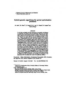
1. Introduction Optimization is essentially the art, science and mathematics of choosing the best among a given set of finite or infinite alternatives. Though currently optimization is an interdisciplinary subject cutting through the boundaries of mathematics, economics, engineering, natural sciences, and many other fields of human Endeavour it had its root in antiquity. In modern day language the problem mathematically is as follows - Among all closed curves of a given length find the one that closes maximum area. This is called the Isoperimetric problem. This problem is now mentioned in a regular fashion in any course in the Calculus of Variations. However, most problems of antiquity came from geometry and since there were no general methods to solve such problems, each one of them was solved by very different approaches. Generally, optimization algorithms can be divided in two basic classes: deterministic probability algorithm. Deterministic algorithm are most often used if a clear relation between the characteristic of possible solutions and their utility for a given problem exists. If the relation between a solution candidate and its fitness are not so obvious or too complicated, or the dimensionality of the search space is very high, it becomes harder to solve a problem deterministically. Trying it would possible result in exhaustive enumeration of the search space, which is not feasible even for relatively small problem. Then, the probabilistic algorithm come in to play. The increased availability of computing power in past two decades has been used to develop new techniques of optimization Today's computational capacity and the widespread Availability of computers have enabled development of new generation of intelligent computing techniques, such as genetic algorithm. Evolutionary Algorithm are population met heuristic optimization algorithms that use biologic- inspired mechanisms like mutation, crossover, natural selection, and survival of the fittest in order to refine a set of solution candidates iteratively [ Weise, 2009]. All evolutionary algorithms proceed in principle according to the scheme illustrated in fig.(1). A simple Genetic Algorithm is search algorithms based on the mechanics of natural selection and neutral genetics. They combine survival of fittest among string structures with a structure yet randomized information exchange to form a search algorithm with some of
220
Evolutionary Algorithms
Evaluation Compute the objective values of the solution candidates Initial Population: Create an initial population of random individual
Reproduction: Create new individuals from the mating pool by crossover and mutation
Fitness Assignment: Use the objective values to determine fitness values
Selection: Select the fittest individuals for reproduction
Fig. 1. Cyclic life of an evolutionary algorithms the innovative flair of human search. In every generation; a new set of artificial creatures (string) is created using bits and pieces of the fittest of the old; an occasional new part is tried for good measure. They efficiently exploit historical information to speculate on a new search points with expected improved performance. A hybrid genetic algorithm (HGA) is the coupling of two processes: the simple and a local search algorithm. HGAs have been applied to a variety of problems indifferent fields, such as optical network design [Sinclair,2000], signal analysis [Sabatini, 2000], and graph problems [Magyar et al, 2000], among others. In these previous applications, the local search part of the algorithm was problem specific and was designed using trial-and-error experimentation without generalization or analysis of the characteristics of the algorithm with respect to convergence and reliability. The purpose of this study is to develop variants of hybrid simple genetic algorithm with local search algorithm represent by gradient or global algorithm present by evolution strategy to optimize solution of some functions where classifies as multimodal function and unimodel functions. One of import function of this study is likelihood function of time series autoregressive moving average 1,1 model, this function defined as a unimodel function it is one of fundamental importance in estimation theory. The other functions used in this study as a test function used widely as benchmark functions. This study presents the( 1) which is represent hybrid of simple genetic algorithm with an widely local search algorithm used steepest decent algorithm the other approach of hybrid denoted by 2 is coupling simple genetic algorithm with global search algorithm multimember evolution strategy, compares its performance with the simple( ), steepest descent algorithm(SDA), multimember evolution strategy ; to study the behaviours many of functions classified as its kind multimodal or unimodel function which is used as test functions. The reminder of this chapter, section 2 presents definitions needed, section 3 giving a brief overview of genetic algorithms, representation of search points and their fitness evolution, selection, recombination, and mutation mechanisms. Then to be consistent, section 4 introduce the characteristic components of local search and its operators , also section 5 issue of the multimember evolution strategy. Section 6 address the issue of coupling simple genetic algorithm with multimember evolution strategy. Section 7 is an
Variants of Hybrid Genetic Algorithms for Optimizing Likelihood ARMA Model Function and Many of Problems
221
extension of the results of section, in which are representative of the classes of unimodel , and multimodal function. In which competition is raised.
2. Definitions Definition 2.1 (Objective Function) An objective function f: with is a mathematical function which is subject to optimization. The co-domain of an objective function as well as its range must be a subset of the real numbers . The domain of f is called problem space and can represent any type of element like numbers, lists, construction plans, and so on. It is chosen according to the problem to be solved with the optimization process. Objective functions are not necessarily mere mathematical expressions, but can be complex algorithms that, for example , involve multiple simulations. Global optimization comprises all techniques that can be used to find with respect to such criteria . the best element of one (objective) function : Definition 2.2 (local Maximum) A local maximum x for all x neighbouring x . If , we can write: is an input element ,|
0:
|
Definition 2.3 (Local Optimum). A (local) minimum x f: is an input element with f x
f x for all x neighbouring x ,
. of one (objective) function ,|
0:
|
.
Definition 2.4 (Local Optimum).A local optimum x of one (objective) function f: is either a local maximum or a local minimum. Definition 2.5 (Global Maximum). A global maximum of one (objective) function f: is an input element with . Definition 2.6 (Global Maximum). A global maximum function f: is an input element with
of one (objective)
. Definition 2.7 (Local Optimum): A global optimum x of one (objective) function f: is either a global maximum or a global minimum. Even a one-dimension function f: may have more than one global maximum, multiple global minimum, or even both in its domain . Take the sine or cosine function for example; for cosine function it has 2 , 0,1,2, … and global minimum 2 1 , 1,2, … . global maximum Definition 2.8 (Solution Candidate): A solution candidate x is an element of the problem space Definition 2.9 (Solution Space): we call the union of all solutions of an optimization problem its solution space . . There may exist This solution space contain (and can be equal to) the global optimal set , especially in the context of constraint valid solution x which are not elements of optimization.
222
Evolutionary Algorithms
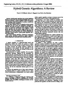
Fig. 2. An example of function with multi global and local maximum and minimum optimal point. Definition 2.10 (Search space ) :The search space of an optimization problem is the set of all elements which can be processed by the search operations. The type of the solution candidates depends on the problem to be solved. Since there are many different applications for optimization, there are many different forms of problem spaces. It would be cumbersome to develop search operations time and again for each new problem space encounter. Definition 2.11 (Genotype): the elements of the search space of a given optimization problem are called the genotypes. The elements of the search space rarely are unconstraint aggregations. Instead, they often consist of distinguishable parts, hierarchical units, or well-type data strictures. The same goes for DNA in biology. It consists of genes, segments of nucleic acid, that contain the information necessary to produce RNA strings in a controlled manner. A fish, for instance, may have a gene for the colour of its scales. This gene, in turn, could have two possible "values" called alleles, determining whether the scales will be brown or grey. The genetic algorithm community has adopted this notation long ago and we can use it for arbitrary search space. Definition 2.12 (Gene). The distinguishable units of information in a genotype that encode the phonotypical properties are called gene. Definition 2.13 (Allele): An allele is a value of specific gene. Definition 2. 14 (Locus): The locus is the position where a specific gene can be found in a genotype. Definition 2.15 (Search Operation): the search operation search OP are used by optimization algorithm in order to explore the search space . Definition 2.16 (individual): An individual p is a tuple p. g, p. x of an element p. g in the search space and the corresponding element . . in the problem space . Definition 2.17 (Population): A population (pop) is a list of individuals used during an optimization process. :
. , .
.
.
Variants of Hybrid Genetic Algorithms for Optimizing Likelihood ARMA Model Function and Many of Problems
223
As already mention, the fitness of an element in the problem space often not solely depends on the element itself. Normally, it is rather a relative measure putting the features of in to the context of a set of solution candidates . 2.1 Genotype-phenotype mapping The genotype –phenotype mapping (GPM, or ontogeny mapping) : is a left-total binary relation which maps the elements of the search space to elements in the problem space ;
Fig. 3. The relation of genome, genes, and the problem space.
3. Genetic algorithm 3.1.1 Initialization The first step is the creation of an initial population of solutions, or chromosomes. The populations of chromosomes generally chosen at random, for example, by flicking a coin or by letting a computer generate random numbers. There are no hard rules for determining the size of the population. Larger populations guarantee greater diversity and may produce more robust solutions, but use more computer resources. The initial population must span a wide range of variable settings, with a high degree of diversity among solutions in order for later steps to work effectively. 3.1.2 Fitness evaluation In the next step, the fitness of the population's individuals evaluated. In biology, natural collection means that chromosomes that are more fit tend to produce more offspring than do those that are not as fit. Similarly, the goal of the genetic algorithm is to find the individual representing a particular solution to the problem, which maximizes the objective function, so its fitness is the value of the objective function for a chromosome. Genetic algorithms can of course also solve minimization problems. The fitness function (also called objective function or evaluation function) used to map the individual's chromosomes or bit strings into a positive number, the individual's fitness. The genotype, the individual's bit string, has to be decoded for this purpose into the phenotype, which is the solution alternative. Once the genotype has been decoded, the calculation of the fitness is simple: we use the fitness function to calculate the phenotype's parameter values into a positive number, the fitness. The fitness function plays the role of the natural environment, rating solutions in terms of their fitness. To apply the GA to real – valued parameters optimization problems of the form : ∏ ,
224
Evolutionary Algorithms
, the bit string is logically divided in to n segments of (in most cases )equal length and each segment is interpreted as the binary code of the corresponding object variable , . A segment decoding function Γ : 0,1 , typically looks like Γ(
∑
….
2
(1)
. …. denotes the ith segment of an individual ... . Associated with each individual is fitness value. This value is a numerical quantification of how good of solution to optimization problem the individual is .Individual with chromosomal strings. Representing better solution has higher fitness values, while lower fitness values attributed to those whose bit string represents inferior solution. Combining …. Γ , the segment-wise decoding function to individual – decoding function Γ Γ fitness values are obtained by setting
where
Γ
(2)
where denotes a scaling function ensuring positive fitness values such that the best individual receives largest fitness. 3.1.3 Selection In the third step, the genetic algorithm starts to reproduce. The individuals that are going to become parents of the next generation selected from the initial population of chromosomes. This parent generation is the "mating pool" for the subsequent generation, the offspring. Selection determines which individuals of the population will have all or some of their genetic material passed on to the next generation of individuals. The object of the selection method is to assign chromosomes with the largest fitness a higher probability of reproduction. 3.1.4 Tournament selection The tournament selection method select times the best individual from a random subset , 2 1, … , and transfers it to the mating pool (note hat there of size | | may appear duplicates). The best individual within each subset selected according to the relation (read: better then). A formal definition of the tournament selection operator : follows (Schowefel &Bäck, 1997): 1, … , be random subsets of each of size| | . 1, … , Let choose such that : where :
Φ
0
Γ
0
Γ
(3)
3.1.5 Genetic operators 3.1.5.1 Crossover The primary exploration operator in genetic algorithms is crossover, a version of artificial mating. If two strings with high fitness values mated, exploring some combination of their genes may produce an offspring with even higher fitness. Crossover is a way of searching the range of possible existing solutions. There are many ways in which crossover can implemented, such as one point crossover, two-point crossover, n-point crossover, or uniform crossover. In the following, we will stay with the simplest form, Holland's one-point crossover technique. Single-point crossover is the simplest form, yet it is highly effective.
Variants of Hybrid Genetic Algorithms for Optimizing Likelihood ARMA Model Function and Many of Problems
225
One point crossover, is often used in , it work first randomly picking a point between 0 ,…. and ,…. are then split and . The participating parent individuals at the point , followed by a swapping of the split halves to form two offspring individual ̀ ̀ as follows (Kargupta, 1995): ,…., ̀ where
1, … ,
,
,
,….,
̀
,….,
,
,
,….,
(4)
1 denotes a uniform random variable .
3.1.5.2 Mutation If crossover is the main operator of genetic algorithms that efficiently searches the solution space, then mutation could called the "background operator" that reintroduces lost alleles into the population. Mutation occasionally injects a random alteration for one of the genes. Similar to mutation in nature, this function preserves diversity in the population. It provides innovation, possibly leading to exploration of a region of better solutions. Mutation performed with low probability. Applied in conjunction with selection and crossover, mutation not only leads to an efficient search of the solution space but also provides an insurance against loss of : formally works as needed diversity, on a single individual , mutation operator ,…, ̀ ,…, ̀ , 1, … , : follows (Back & Schwefel, 1993): ̀ where
,χ ,χ
x 1
x
P P
(5)
0,1 is a uniform random variable, sampled anew for each bit.
3.1.6 Conceptual algorithm The conceptual algorithm of can then formulated as t:=0; t is the generation number 0 ,…, 0 Where 0,1 Initialize 0 0 ,…,Φ 0 Evaluate 0 Φ 0
Where Φ While Recombine:
̀ "
Mutate: Evaluate Where
Γ 0 , 0 do // while termination criterion not fulfilled 1, . . , "
Φ
" "
0
̀ ,…, Γ
1, . . , } "
: Φ "
"
,…,Φ
,
"
;
end Fig. 4. Pseudo code of
algorithm
3.2 Theorems and definitions needed Definition 2.1 The directional derivatives of f(x, y) at the point (a, b) and in the direction of the unit vector u u , u is given by D f a, b
lim
,
,
(6)
226
Evolutionary Algorithms
provided the limit exists. Theorem 2.1 Suppose that f is differentiable at (a, b) and u D f xa, b
u ,u
is any unit vector. Then we can write
f a, b
f a, b
(7)
Clearly 2.1 For convenience, we define the gradient of a function to be vector –valued function whose component are the first –order partial derivatives of f . we denote the gradient of a function f by grad of f or f read "del f" and define by the given theorem . Theorem 2.2 If f is a differentiable function of x and y and u is any unit vector, then ,
,
.u
(8)
Clearly 2.2 This theorem clear how to compute directional derivatives. Further, writing directional derivatives as a dot products. This theorem generalized to vector valued : . Theorem 2.3 Suppose that f is differentiable function of x and y at the point , . Then i. the maximum rate of change of f at , is f a, b and occurs in the direction . ii.
of the gradient,
, ,
the minimum rate of change of f at (a, b) is ,
and occurs in the direction opposite the gradient u
,
,
.
iii. the gradient f a, b is orthogonal to the level curve f x,y)=c at the point (a ,b), where c=f(a, b). Definition 2.2 We call f(a, b) a local maximum of f if there is an open disk R centred at (a, b), for which f a, b f x, y for x, y R. Similarly , f(a, b) is called a local minimum of f if there is an open disk cantered at (a, b), for which f a, b f x, y for x, y R. In either case f(a, b) is called a local extreme of f. Theorem 2.4 suppose that f(x,y) has continuous second order partial derivatives in some open disk containing the point (a ,b) and that f a, b f a, b 0. Define the discriminant D for the point , by D a, b if
,
0 and f , if , if ,
if
f
a, b f
f
a, b
a, b 0, then f has a local minimum at , . 0, then f has a local maximum at 0 and f a, b 0 , then f has a saddle point at , . 0, then no conclusion can be drawn.
(9) ,
.
4. Local search The local search operator looks for the best solution starting at a previously selected point, in this case a solution in the population. For this application, the steepest descent method was chosen as the local search operator. This method moves along the direction of the steepest gradient until an improved point found, from which a new local search starts.
Variants of Hybrid Genetic Algorithms for Optimizing Likelihood ARMA Model Function and Many of Problems
227
The algorithm ends when no new relationship shown point can found (this is equivalent to a gradient equal to zero). For functions with multiple local optimum, the method find one local optima but it is not guaranteed to find the global minimum. For geometric with conical shape, for example, the method finds the local optimum in one local search starting from any point in side the basin of attraction. For other geometries, the local search operator required more than one iteration to achieve the solution. 4.1 Descent method Cauchy (1847), Kantorovich (1940-1945), Leven berg (1944), and Curry (1944) are the originators of the gradient strategy, which started life as a method of solving equations and systems of equations. It first referred to as aid to solving variation problems by Hadamard (1908) and Courant (1943). This variant of the basic strategy, known under the name optimum gradient method, or method of 'steepest descent'. Theoretical investigations of convergence and rate of convergence of the method can be found e.g. in Akaike (1960),Goldstein (1962), Ostrowski (1967), Zangwill(1969) and Wolfe(1969,1970,1971)[6] The general rule of steepest descent where used to find optimal solutions of nonlinear problems is x
x
α d
(10)
Where d is an a suitably chosen direction and α is a positive parameters (called step-size) that measures the step along the direction d . This direction is a descent direction if d d
T
f x 0
0
x if
f x
0 0
(11)
4.1.1 Steepest descent algorithm To approximate a solution p to the minimization problem G p min R G x Given an initial approximation x: Step 1. set k 1 Step 2. While k N do steps ( 3-8 ) G x , … , x // note: g G x ; Step 3. Set g G x ; z G x , … , x // note: z z ||z|| Step 4. if z 0 then output ("zero Gradient'') Output (x , … , x , g //[Procedure completed may have minimum check further] Step 5. choose δ s.t δz g min G x Step 6. Set x x δz Step 7. if |g g | then output x , … , x , g // [ Procedure completed successfully ] Stop Step 8. set k=k+1; Step 9. Output ('Minimum Iterations Exceeded') // ( Procedure completed unsuccessfully ) Stop Fig. 5. Pseudo code of gradient algorithm
228
Evolutionary Algorithms
4.2 Hybrid genetic algorithm In this section we define a hybrid of with gradient method and we denoted as (HGA1) A hybrid genetic algorithm (HGA) is the coupling of two processes: the simple and a local search algorithm. The local search part of the algorithm was problem specific and designed using trial-and-error experimentation without generalization or analysis of the characteristics of the algorithm with respect to convergence and reliability. The HGA algorithm is a standard, which combines an with local search. The local search step defined by three basic parameters: frequency of local search, probability of local search, and number of local search iterations. The first element for the definition of the algorithm is the frequency of local search, which is the switch between global and local search. In the algorithm, this switch performed every "G!" global search generations, where "G!" is a constant number called the local search frequency. The second element of the algorithm is the probability of local search P, which is the probability that local search will be performed on each member of the population in each generation where local search is invoked. This probability is constant and defined before the application of the algorithm. Finally, each time local search is performed, it is performed a constant number of local search iterations before local search is halted. 4.2.1 Basic elements 4.2.1.1 Genetic algorithm Three basic operators define the simple Genetic Algorithm ( ): binary tournament selection, single point crossover, elitism, and simple mutation. Through the successive application of these three operators, an initial population of solutions evolved into a highly fit population. 4.2.1.2 Local search The local search operator looks for the best solution starting at a previously selected point, in this case a solution in the SGA population. For this application, the steepest descent method was chosen as the local search operator. This method moves along the direction of the steepest gradient until an improved point found, from which a new local search starts. The algorithm ends when no new relationship shown point can found (this is equivalent to a gradient equal to zero) and this satisfied in our formula adaptation [10]. 4.3 Hybrid genetic algorithm with local search algorithm A hybrid genetic algorithm (HGA) is the coupling of two processes: the and a local search algorithm. The local search part of the algorithm was problem specific and was designed using trial-and-error experimentation without generalization or analysis of the characteristics of the algorithm with respect to convergence and reliability. It is defined by three basic parameters: frequency of local search, probability of local search, and number of local search iterations. The first element for the definition of the algorithm is the frequency of local search, which is the switch between global and local search. In the HGA1 algorithm, this switch performed every "G!" global search generations, where "G!" is a constant number called the local search frequency. For example, if G!=3, local search would perform every 3 generations during the . The second element of the algorithm is the probability of local search P, which is the probability that local search will be performed on each member of the population in each generation where local search is invoked. This probability is constant and defined before the application of the algorithm. Finally, each time local search performed; it performed for a constant number of local search iterations before local search halted.
Variants of Hybrid Genetic Algorithms for Optimizing Likelihood ARMA Model Function and Many of Problems
229
4.3.1 Conceptual algorithm of The coupling approach in this paper consist in the introduction of generation interval for hybrid activation operator (HAO).Through selection, crossover, and mutation operators, the canonical works on population of bit string encoding scheme generation by generation. When HAO is active (again implemented here every G? generation), the intermediate generation created by GA is fed into an adopted selection strategy which select subpopulation, usually of small size. Then each binary string individual in this subpopulation is convert into a real number vector, to be the initial value of steepest descent ( ) algorithm that operate on this subpopulation for fixed small of generation. The vectors converted back into bit string values to manipulate again by master GA, used here in this hybridization as a tool operates in small number of generation fashion in an order to enhance the selected points driven from the master GA. It is appropriate that the version of tools to be of preservative survivor property to have worthy adjustment. The conceptual algorithm of the (HGA) given by the following steps: Input: sample size, number of generation, .. Output approximate value Step1: Initialize GA generate Initial population of parameters . Step2.1: for t 1to number of generation Do Step2.2: for I 1: population size Do The canonical genetic algorithm sGA operators: Step2.2.1: Local Recombination, Step2.2.2: Mutation, Step2.2.3 Selection, Step3: Binary coded sGA individual remapped in to real vector individual. 1 Step4.1: Select of population size use as initial solution of sDA perform for each generation 3 Step4.2. Start local search evaluation// Starting of Steepest Descent Algorithm sDA . Step4.3. : Real _coded local search algorithm individual remapped in to binary vector individual. Step5. Repeat steps until all of generation complete or termination criterion is satisfied. Step6: end Fig. 6. Pseudo code of HGA algorithm
5.
,
-Evolution strategies
H.-P. Schwefel proposed the multi-member evolution strategies, the so-called , their most general form, these strategies are described in the coming subsections.
-ES. In
5.1 Representation and fitness evaluation , -ES can consist of the components (Robert, Roland, 2002): An individual , in : The vector of object variables. : A vector of step length or standard deviations 1 of the normal distribution. The strategy parameter (also called the internal model) determines the variances of the n-dimensional normal distribution, which is used for exploring the search space. The user of an evolution strategy, depending on his feeling about the degree of freedom required, can vary the amount of strategy parameters attached to an individual. As a rule of thumb, the global search reliability increases at the cost of computing time when
230
Evolutionary Algorithms
the number of strategy parameters is increased. The setting most commonly used which form the extreme cases are: 1 : (Uncorrelated mutation with one single standard deviation controlling • mutation of all components of ). : (Standard mutations with individual step sizes , . . , controlling mutation of • individually). The only part of entering the the corresponding object variables objective function evaluation is , and the fitness of an individual is identical to its objective function value , i.e. ). 5.2 Mutation operator The generalized structure of , -ES mutation operator consists of the addition of a normally distributed random number to each component of the object variable vector, corresponding to a step in the search space. The variance of the step-size distribution is itself subject to mutation as a strategy variable. Formally speaking, mutation operator , : , is defined as follows [5] ,
,
Which proceeds by first mutating the strategy parameters exp
,…,
:
(13) :
exp
; (14)
, ~ 0, 1, … . , Where ~ 0, To prevent standard deviations from becoming practically zero, a minimal value of is algorithmically enforced for all . Secondly, modifying according to the new set of strategy parameters obtained from mutating : : ,…,
(15)
5.3 Recombination operators , -ES, different recombination mechanisms are used in either local form, producing In one new individual from two randomly selected parent individuals, or in global form, allowing components to be taken for new individual from potentially all individuals available in the parent population. Furthermore, recombination is performed on strategy parameters as well as the object variables, and the recombination type may be different for object variables, and standard deviations. Depending on the recombination types [4][6]:
=
0 1 2 3 4
No recombination Discrete recombination of pair of parents Intermediate recombination of pair of parents Discrete recombination of all parents Intermediate recombination of parents in pairs
(16)
Sometimes, the choice of a useful recombination operator for a particular optimization problem is relatively difficult and requires performing some experiments [2].The rules of for creating an individual, , recombination operator :
Variants of Hybrid Genetic Algorithms for Optimizing Likelihood ARMA Model Function and Many of Problems
231
, , are given respectively by referring to arbitrary vectors and where and denote here the part (i.e., either or ) of a pre-selected parent individuals and the part of an offspring vector receptively. Each of and are of length , , 1, … ,
,
=
0 1 2 3 4
, ,
,
. 0.5
,
,
. 0.5
,
Where
,
~
1, … ,
for each offspring, and
,
~
1, … ,
(17)
for each .
5.4 Selection operator There are two main classifications for selection according to the survival property of the parents [6]: Extinctive_ , strategy; where parents live for a single generation only. : where | | &| | : : ,& Preservative_ strategy; where selection operates on the joined set of parents and offspring, i.e., very fit individuals may survive indefinitely: : where | | ,&| | , , and : : The ratio is known as selection pressure. In the choice of and , there is no need to ensure that is exactly divisible by . The association of offspring to parents is made by a random selection of evenly distributed random integers from the range 1, . It is only necessary that exceeds by a sufficient margin that on average at least one offspring can are tuned for a be better than its parent. Hoffeister and Bäck in [7] have stated that maximum rate of convergence, and as a result tend to reduce their genetic variability, i.e., the number of different alleles (specific parameter setting) in a population, as soon as they are attracted by some local optimum.
6. Cross- fertilization space of conical GAS and Standard Variant
,
-ES
The coupling approach followed in this section consists in the introduction of generation interval for hybrid activation operator(HAO). Through selection , crossover, and mutation operators, the simple GA works on population of bit string encoding scheme generation by generation. When HAO is active ( implemented for every G? generation ), the intermediate generation created by is fed into adopted selection strategy which select ub population, usually of small size. Then each binary string individual in this subpopulation is converted in to a real number vector , to be the parents of the first generation of ES tool that operate on this subpopulation for a fixed small number of generations. The vectors are converted back in to bit string values to be manipulated a gain by the master . As is used here in this hybridization as a tool operator in a small number of generation fashion in an order to enhance the selected point driven from the master , then it is appropriate that the version of the ES too is to be of preservative survivor property to have worthy adjustment i.e., a , -ES is used.
232
Evolutionary Algorithms
t=0; {is the generation number} ls=tmax {is the HAO age} Initialize 0 0 ,…, 0 where I 0,1 ; 0 ,…,Φ Evaluate 0 Φ where Φ a 0
δ f Γ a 0
0,1
Where 0
,P 0
;
while (τ P t true do {while termination criterion not fulfilled} rp P t recombine: a" t k 1, … . , µ ; mutate: a" t mp k 1, … . , µ ; a t evaluate P" t a" t , … a"µ t : Φ a" t , … Φ a"µ t : where Φ a" t δ f Γ a" t , P t w ; if ls 0 do if HAO still live and active Select :P pop t b t , … bµ t Iµ and Where I R b t x ,σ i 1…n j 1, … n ; {binary _coded GA individual is remapped in to (µ λ ES {real vector individual} For t µ 1 to t ES _ µ ES {do tmax sexual propagation Recombine : b " t Mutate: b " t
µ
Evaluate : P " t Φ b" t
µ
t
t Where I
, … , a"
ES
f
µ
t
t I
k
1, … , λ t
ES ;
µ
ES
µ
x"
P
1, … , λ ;
ES , … , b "
t
ES ;
µ
ES S P tµ ES generation loop P
k ES
µ
, … , Φ b" t
µ
Select: P t µ End µ1 λ1 Evaluate P" t P" t a"
P t b tµ
,
b" t
ES
ES b"
m
ES
µ
Where Φ
r rec , rec
P" t
ES
_ µ
µ
ES
ES
µ
0,1
and Φ a" t
δ f Γ a" t
,P t
w
; re-evaluate fitness
end Select P t 1 S P" Iµ ls ls 1; when ls=0 then the loop is turned into pure GA phase t t 1 end
Fig. 7. Conceptual algorithm of HGA2 ( hybrid Genetic algorithm with multimember evolution strategy)
Variants of Hybrid Genetic Algorithms for Optimizing Likelihood ARMA Model Function and Many of Problems
233
7.2 Test functions In order to evaluate the behaviours of hybrid genetic algorithms, a set of test problem have been carefully selected to illustrate the performance of the algorithms and to indicate that it has been successful in practice. The nine test functions, which is classifies as multimodal or unimodel function; these function given with more details in section below. 7.3 Simulations Multi- functions used as a test functions classified as unimodel and multi model it is deployed to verify the proposed hybrid genetic algorithms. The firs test function is likely hood function of ARMA(1,1) model, this function classifies as a unimodel the simulating experiment described in the following. 7.3.1 : Test function / Likelihood function The likelihood function is one of fundamental importance in estimation theory. This principle says that the data has to tell us about the parameters contained in the likelihood function, all other aspects of the data being irrelevant. In moderate and large samples, the likelihood function will be unimodel and can be adequately approximated over a sufficiently extensive region near the maximum by a quadratic function. Hence, in these cases the log-likelihood function can be described by its maximum and its second derivatives at the maximum. The values of parameters which maximize the likelihood function, or equivalently the loglikelihood function, are called maximum likelihood (ML) estimates. The second derivatives of the log –likelihood provide measurers of “spread” of the likelihood function and can be used to calculate approximate standard errors for the estimates [ ]. Now, to study the likelihood function of 1,1 let as suppose the original ,..,Z Z ,Z ,..,Z observations from a time series which can be denoted by Z we assume that this series is generated by an 1,1 model. From these observations, we can generate a series w of n N d differences , , . . , , where . The stationary mixed 1,1 model in eq.7 may be written as [2]: (18) Where 0. Suppose that has the normal distribution with zero mean and constant variance equal to σ , then the likelihood function can get as follows [2]: |
2 Where
,
,
,
,
| exp
(19)
, ,
,
(20)
,
(21)
then the log- likelihood function is: ln L
2πσ
ln M
,
S
,
(22)
234
Evolutionary Algorithms
where: ∑
,
|
,
,
(23)
| , , is the sum squares errors, is the sample size, and | , , conditional on , and . Sum squares errors can be found denotes the expectation of by unconditional calculation of the are computed recursively by taking conditional expectations in eq.13. A back-calculation provides the values , 0,1,2, .. This back-forecasting needed to start off the forward recursion. , /2 and thus the For moderate and large values of n in eq.17 is dominated by , contours of the unconditional sum squares function in the space of the parameters are very nearly contours of likelihood and of log likelihood . It follows, in particular, that the parameter estimates obtained by minimizing the sum of squares in eq.17, called least square estimates will usually provide very close approximation to the (maximum likelihood estimator). 7.3.1.1 Drive formula of gradient of likelihood function These section, we try to drive general form of steepest descent to estimate 1,1 model parameters, is an iterative strategy depends on the following rule for numerical computation: β
β
k e
(24)
Where Parameter model Constant value depend is the gradient which approximate by e
,
,…,
we can see that the estimation of parameters depend on iterative algorithm which start (get by one of traditional estimation methods) this algorithm continue with initial value in modified these estimators even we get the value which don’t have change in values ∑ ̂
(25)
where , actual value of observed time series; ̂ predicted value of actual value. We know, ARMA(1,1) model form is (26) Where s are a random variable with standard normal density function known as random shock term. then (27) ∂a ∂
2a z
,
∂a ∂θ
2a a
S0 ,
2 az
,
2
(28)
Variants of Hybrid Genetic Algorithms for Optimizing Likelihood ARMA Model Function and Many of Problems
235
The value of k gets as follows (29) (30)
0
|Δ |
|
|
2
)
|
1
0
2
)