Back to the Future: Variants of Temporal Defeasible Logic for Modelling Norm Modifications Guido Governatori
Monica Palmirani, Antonino Rotolo Regis Riveret, Giovanni Sartor
School of ITEE University of Queensland, Australia
CIRSFID and Law Faculty University of Bologna, Italy
[email protected]
{palmiran,rotolo,rriveret,sartor}@cirsfid.unibo.it
ABSTRACT This paper proposes some variants of Temporal Defeasible Logic (TDL) to reason about normative modifications. TDL is able to represent them and to deal with conflicts between temporalised normative modifications and other phenomena such as retroactivity. The variants of TDL are defined according to several criteria. For example, we may have logics where rules, conclusions, and modifications persist over time either across repositories or only within repositories. This makes it possible to differentiate cases in which, for example, modifications at some time change legal rules but their conclusions persist afterwards from cases where also their conclusions are blocked.
1.
efficacy or date of application of the destination normative provision (the entire act or a part of it, such as an article or a paragraph); and 4. normative-system changes, which apply not only to specific documents but to the normative system considered in its entirety. In line with the preliminary investigation developed in [7], this work aims to provide a more general treatment in TDL of norm changes over time. The issues discussed in this paper are similar to those assumed in [7], namely: 1. to reason about conditional modifications of conditional normative provisions, where the former ones apply under, and are conditioned to, the occurrence of some uncertain events;
INTRODUCTION
In a successful sequel of movies in the late 80s and early 90s a slightly mad scientist Emmett “Doc” Brown (Christopher Lloyd) invents the “flux capacitator” a device that makes time travel possible, and his young friend Marty McFly (Michael J. Fox) travels to the past and to the future. In particular Marty travels to the future to change the past and to the past to change the future. Despite that time travelling is mainly a popular science fiction topic and many elaborate physical theories have been advanced about the possibility and the consequences of time travelling, there is a field, namely norm modifications, where “time travelling” is very common. This paper presents some variants of Temporal Defeasible Logic (TDL) [7, 6] to reason about different aspects of norm modifications. In general, we may have different types of modification according to how they affect the law. The impact might concern, e.g., the law text, its scope, or the time of its force, efficacy, or applicability. In general, we can identify at least four categories of modifications [15]:
2. to identify criteria for detecting and solving conflicts between textual modifications; 3. to clarify the specific role played by the temporal dimension in modelling norm modification processes.
1. textual changes, which intervene when a legal provision is repealed, replaced, integrated or relocated;
The novelty of this work is that we are interested in defining different temporal constraints according to which the elements of a normative system, and the conclusions that follow from them, can, or cannot persist over time. Indeed, several options are available, and each of them corresponds to a specific way through which norm modifications can take place and behave. The layout of the paper is as follows. In Section 2 we discuss the general conceptual model behind the framework and focus on some specific problems of norm-modifications processes. Section 3 provides an outline of basic Defeasible Logic. Section 4 describes the formal language and define in detail the proof theory of TDL. Section 5 discusses four types of norm modifications in TDL and states when modifications are in conflict. A final section of conclusion completes the paper.
2. change of the norm scope, which might be consequent on derogation, extension, or interpretation;
2.
3. temporal changes, which impact on the date in force, date of
Permission to make digital or hard copies of all or part of this work for personal or classroom use is granted without fee provided that copies are not made or distributed for profit or commercial advantage and that copies bear this notice and the full citation on the first page. To copy otherwise, to republish, to post on servers or to redistribute to lists, requires prior specific permission and/or a fee. ICAIL ’07 Palo Alto, California USA. Copyright 2007 ACM ...$5.00.
NORMATIVE SYSTEMS AND MODIFICATIONS
Norm applications and modifications take place along the axis of 0 time. In particular, a rule is represented at least as (at ⇒ bt ) : t 00 , where instants t and t 0 indicate the time at which a and b hold, while t 00 is the time when the rule is in force. A temporal model should allow us to give an accurate account of the dynamics of norms and therefore to manage legal modifications consistently with legal principles [15]. A legal system is defined as a set of documents fixed at a defined time t and which have been issued by an authority and whose validity depends on rules that determine, for any given time, whether
a single document belongs to the system. Formally: LS(t) = D1 (t), D2 (t), D3 (t), . . . , Dm (t)
(1)
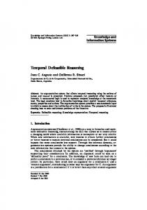
where m ∈ N, Di denotes documents and t is a fixed time in a discrete representation. A normative system, in turn, takes the documents belonging to a legal system and organises them to reflect their evolution over time. A normative system should therefore be more precisely defined as a particular discrete time-series of legal systems that evolves over time. In formal terms: NS = LS(t1 ), LS(t2 ), LS(t3 ), . . . , LS(t j )
• persistent rules, which, if applicable, permit to infer literals that persist unless some other, subsequent, and incompatible events or states of affairs terminate them. • co-occurrent (or transient) rules, which allow for the inference of literals which hold on the condition and only while the antecedents of these rules hold. The above characterisation of transiency and persistency provides only a partial picture of how things can or cannot evolve over time. Persistency is indeed a notion which need to be linked a specific temporal perspective. Consider the following legal provisions r1 : (a10 ⇒ b10 ) : 10 r2 : (b10 ⇒ c10 ) : 10
where j ∈ N. t0
t0 t0
t 00
t0
t 00
LS(t 0 )
LS(t 00 )
t0
t 00
t0
Figure 1: Normative System with Legal Systems at t 0 and t 00 The passage from a legal system to another legal system is effected either by normative modifications or by simple persistence. However, norm-modifying provisions, too, belong to legal systems, and, as other legal provisions, they can be seen as conditional statements. Accordingly, also modifications have three temporal dimensions, these being attached to the conditions, to the effects, and to the overall conditional. These temporal dimensions refer, then, to the efficacy, applicability, and force of the provision, respectively. Furthermore, one has to consider the time of observability of the normative system. Consider a law r of 2001 nullified in 2005: the change affects the entire normative system because the legal text is removed from the system as if it had never been there in the first place (ex-tunc removal). The same would happen with a temporary law decree that does not pass into law, or with a retroactive abrogation, or with an interpretation of a law that comes in as the authentic reading of it [10, 14]. The peculiarity of system changes shows up when we query the system to retrieve information from it: if today (e.g., 2005) we ask for all the laws in force in 2001, law r will not turn up and the system will look as if that law had never been in force in the first place. But if we enter the query as if we were in 2001, when the annulment had not yet occurred, law r will show up as being in force, and the entire system will reflect that fact. This difference depends on the temporal point of view from which we query the system and this refers to the time of observability of a normative system. Indeed, it is possible to distinguish among different kinds of normative conditional in a temporal setting, and so different ways of how normative modifications temporally affect the normative system. Here we will assume to work with the following basic types of normative rules [8, 7]:
Both r1 and r2 are assumed to produce persistent conclusions, namely, that b and c persist after 10 if r1 and r2 are applicable at 10. Now suppose that a modification m at time 20 applies to r1 , holding 10, and nullifies it. This is a case of retroactive modification, as the norm-modifying provision m is in force at 20. If we obtain a at 10, this makes r2 applicable, thus deriving c at 10 and afterwards. So, despite, the annulment of r1 , its legal effects are propagated. A simple solution to obviate the problem is to state that the conclusion of r1 can be propagated after a certain time only if r1 has not been in the meantime nullified. This is not enough, as this would simply block b from 20 afterwards, but it would not apply to c, which was derived at 10: c will hold after 20 independently of m. Of course, we can imagine scenarios in which the applicability of r1 may support a large number of rule chains, thus posing a serious computational problem. Indeed, this is a concrete difficulty which arises when we aim to model ex-tunc modifications which are meant to cancel all legal effects of a certain legal provision. But things are even more complex. In fact, persistency and transiency can apply not only to conclusions of rules, but also to the rules themselves, to the time of observability, and also to derivations (i.e., queries). This give rise to several options regarding how modifications affect the legal system over time, since, as it was said, legal modifications are represented as rules. We will consider the interplay among the following different time-lines: • a time line through which conclusions persist within a certain version of the legal system; • a time line through which derivations persist within a certain version of the legal system; • a time line through which rules persist within a certain version of the legal system; • a time line through which conclusions persist across different temporal versions of the legal system; • a time line through which derivations persist across different temporal versions of the legal system; • a time line through which rules persist across different temporal versions of the legal system. A final note. In the remainder, we will also distinguish between modifiable and non-modifiable rules. Non-modifiable normative provisions are important when constitutions are considered. In fact, in many legal systems some parts of the constitution cannot be changed even by the special procedures the constitution sets forth for its revision. In Italy, for example, this holds explicitly for the political makeup of the state, since article 139 makes it a prohibition to deviate from its republican (and democratic) form.
Again, article 2 qualifies some basic rights as inviolable, even if no explicit reference is made to the legal impossibility of constitutional revisions. This impossibility was subsequently recognised by some decisions pronounced by the Constitutional Court (e.g., no. 18/1982 and no. 1146/1988).
3.
DEFEASIBLE LOGIC
The application we are working on are designed to provide practitioners with advice generated by inference mechanisms that comply with legal principles. The input is the normative information contained in the system and is formalised into an expressive logic, namely, in TDL, which is an extension of Defeasible Logic (DL). The legal temporal model points out the importance of defeasibility due to the addition of new premises that can invalidate formerly derivable consequences. This means that norm modifications must proceed on the basis of defeasible reasoning. In fact, the reasoning used in this context forms part of the wider domain of legal reasoning, which too is deemed to be defeasible [16]. Defeasible reasoning is supported by a number of logics. Among these, DL [12, 13, 2] is based on a logic programming-like language and it is a simple, efficient but flexible non-monotonic formalism capable of dealing with many different intuitions of non-monotonic reasoning. An argumentation semantics exists [5] that makes its use possible in argumentation systems [17]. DL has a linear complexity [11] and also has several efficient implementations [4]. We have three types of rules in DL: strict rules, defeasible rules and defeaters. A rule expresses a relationships between a set of premises and a conclusion, and the three types of rules convey the strength of the relationships. A strict rule states the strongest kind of relationship since the conclusion always holds when the premises are indisputable. Defeasible rules cover the case when the conclusion normally holds when the premises tentatively hold; finally defeaters consider a situation where the premises do not warrant the conclusions: in defeaters the premises simply prevent another rule to support the opposite. Accordingly, a conclusion can be labelled either as definite or defeasible. A definite conclusion is an indisputable conclusions, while a defeasible conclusion can be retracted if additional premises become available. DL is based on a constructive proof theory based for conclusions. Accordingly we can say that a derivation for a conclusion exists and that it is not possible to give a derivation for a conclusion. Based on these two ideas we will label the conclusions according to their strength and type of derivation, and we have four possibilities: • +∆p, meaning that we have a definite proof for p (a definite proof is a proof where we use only facts and strict rules); • −∆p, meaning that it is not possible to build a definite proof for p; • +∂ p, meaning that we have a defeasible proof for p; • −∂ p, meaning that it is not possible to give a defeasible proof for p. In what follows we will refer to +∆, −∆, +∂ and −∂ as proof tags, and we will give formal conditions under which we can label a conclusion with one these proof tags. These different notions of provability come of use here because they enable the system to label a suggestion as stronger or weaker depending on the kind of proof associated with it. Strict proofs are just derivations based on detachment (Modus Ponens) for strict rules. Given a strict rule a1 , . . . , an → b, where we have definite proofs for all ai ’s, we can deduce b.
DL is a sceptical non-monotonic formalism. This means that if a possible conflict between two conclusions (i.e., one is the negation of the other), DL refrains to take a decision and we deem both as not provable unless we have some more pieces of information that can be used to solve the conflict. One way to solve conflicts is to use a superiority relation over rules. The superiority relation gives us a preference over rules with conflicting conclusions. In case we have a conflict between two rules we prefer the conclusion of the strongest of the two rules. The superiority relation is applied in defeasible proofs. Defeasible proofs are structured in three phases: in the first phase we look for an argument supporting the conclusion we want to prove. More precisely we want an applicable rule for the conclusion. In the second phase we look for arguments/rules for the opposite of what we want to prove. In the last phase we rebut the counterarguments. This can be done by showing that the counterargument is not founded (i.e., some of the premises do not hold), or by defeating the counterargument, i.e., the counterargument is weaker than an argument for the conclusion we want to prove. In other words, a conclusion p is derivable when: • p is a fact; or • there is an applicable strict or defeasible rule for p, and either – all the rules for ¬p are discarded (i.e., not applicable) or – every applicable rule for ¬p is weaker than an applicable strict or defeasible rule for p. Notice that a strict rule can be defeated only when its antecedent is defeasibly provable.
4.
TEMPORAL DEFEASIBLE LOGIC
DL allows us to deal with incomplete information but as such does not provide any mean to deal with temporal aspects. Temporal Defeasible Logic is an umbrella expression to designate extensions of Defeasible Logic to capture time. TDL has proved useful in modelling temporal aspects of normative reasoning, such as temporalised normative positions [8]; in addition, the notion of a temporal viewpoint –the temporal position from which things are viewed– allows for a logical account of norm modifications and retroactive rules [7]. We present in this section some variants that deal with temporal dimensions as exposed in the legal temporal model (see Section 2). Temporal aspects are integrated by two means: first by introducing temporal coordinates and second normative modifications. [8] extended DL with temporalised literals, i.e., every literal in the logic has associated to it a timestamp. Thus we have expressions of the type a : t, meaning that a holds at time t. This means that we have to give the condition to prove a literal at time t. So besides the straightforward extension of the conditions given above, we have to consider whether a conclusion is transient (holding at precisely one instant or time) or whether it is persistent. To prove that a holds at t, we can prove that a held at a previous instant t 0 and then for all instant in between t and t 0 , it is not possible to terminate a. We will refer to this property as persistence of a conclusion. As we have argued above not only literals (propositions) have their temporal validity, but this is true for the other components of our knowledge: we can speak of the time of force a rule, i.e., the time when a rule can be used to derive a conclusion given a set premises. In this perspective we can have expressions like r : (ata → btb ) : tr
(2)
meaning that the rule r is in force at time tr , or in other words, we can use the rule to derive the conclusion at time tr . The full semantics of (2) is that at time tr we can derive that b holds at time tb if we can prove that a holds at time ta . But now we are doing a derivation at time tr , so the conclusion btb is derived at time tr and the premise ata must be derived at time tr as well. In the same way a conclusion can persist, and we can have the same for rules and then for derivations. Let us consider the following example from a hypothetical taxation law. If the taxable income of a person at January 31, for the previous year are in excess on 100,000$, then the top marginal rate computed at February 28 is 50% of the total taxable income. And this provision is in force from January 1. This rule can be written as follows: T hreshold 31Jan ⇒ HighMarginalRate28Feb : 1Jan Let us suppose that the last instalment for the salary was paid to an employee on January 4, and that it makes the total taxable income greater than the threshold stated above. We used T hreshold 4Jan to signal that the threshold of 100,000$ has been certified on January 4. Clearly T hreshold 4Jan is a persistent property, thus in this case we can derive that the threshold was reached by January 31. So let us ask what the top marginal rate for the employee is if she lodges a tax return on January 20. What we have to do is to see whether the rule is still in force on January 20. Given that the norm was valid from January 1, and no changes were made to the legislation in between, the rule persists. Thus from the point of view of January 20, the top marginal rate is 50%. Suppose now that there is a change in the legislation and that the above norm is changed on February 15, and the change is that the top marginal rate is 30%. T hreshold 31Jan ⇒ MediumMarginalRate28Feb : 15Feb In this case if the employee lodges her tax return after February 15, the top marginal rate is 30% instead of 50%. From the above example it is clear that what we derive depends on what rules are valid, and on the normative content of rules, at the time when we do the derivation. In addition the above example illustrates the case that the content of a rule can be changed. Thus we have to devise a mechanism to capture this phenomenon. To this end we introduce meta-rules, i.e., rules where the consequent is itself a rule and not only a simple proposition. In addition to keep track of the changes to a norm, i.e., to represent a normative systems as defined in Section 2, we introduce the notion of a repository, i.e., a snap-shot of rules and literals known to exist at a specific time instant. In the rest of the section we will give a formal presentation of the notions discussed so far.
4.1
Language
The language of TDL is based on a (numerable) set of atomic proposition Prop = {p, q, . . .}, a set of rule labels {r1 , r2 , . . .}, a discrete totally ordered set of instants of time T = {t1 ,t2 , . . . }, and the negation sign ¬. A plain literal is either an atomic proposition or the negation of it. Given a literal l with ∼l we denote the complement of l, that is, if l is a positive literal p then ∼l = ¬p, and if l = ¬p then ∼l = p. If l is a literal and t is an instant of time, i.e., t ∈ T , the l t is a temporal literal. We will use TLit to denote the set of temporal literals. Intuitively the meaning of a temporal literal l t is that l holds at time t. Knowledge in DL can be represented in two ways: facts and rules. Facts are indisputable statements, represented either in form of states of affairs and actions that have been performed (literals). For example, “John is a minor in year 2007”. In the logic, this might be expressed as Minor(John)2007 .
A rule is a relation between a set of of premises (conditions of applicability of the rule) and a conclusion. In this paper the admissible conclusions are either literals or rules themselves; in addition the conclusions and the premises will be qualified with the time when they hold. We consider two classes of rules: meta-rules and proper rules. Meta-rules describe the inference mechanism of the institution on which norms are formalised and can be used to establish conditions for the creation and modification of other rules or norms, while proper rules corresponds to norms in a normative systems. As we have previously discussed, beside the above classification, rules can be partitioned according to their strength into strict rules (denoted by →), defeasible rules (denoted by ⇒) and defeaters (denoted by ;). Strict rules are rules in the classical sense: they are monotonic and whenever the premises are indisputable so is the conclusion. Defeasible rules, on the other hand, are nonmonotonic: they can be defeated by contrary evidence. Finally defeaters are the weakest rules: they do not support conclusions, but can be used to block the derivation of opposite conclusions. Thus we define the set of rules using the following recursive definition: • a rule is either a meta-rule or a proper rule or the empty rule ⊥, where • If r is a proper rule then ∼r is a rule. • If r is a rule and t ∈ T , then r : t is a temporalised rule. (The meaning of a temporalised rule is that the rule is in force at time t). • Let A be a finite set of temporal literals, C be a temporal literal and r a temporalised rule, then A ,→ C is a rule, and A ,→ r and A ,→ ∼r are meta rules (henceforth we use ,→ as a meta-variable for either → when the rule is a strict rule, ⇒ when the rule is a defeasible rule, and ; when the rule is a defeater). Given a set R of rules, we denote the set of all strict rules in R by Rs , the set of defeasible rules in R by Rd , the set of strict and defeasible rules in R by Rsd , and the set of defeaters in R by Rd f t . R[q] denotes the set of rules in R with consequent q. For a rule r we will use A(r) to indicate the body or antecedent of the rule and C(r) for the head or consequent of the rule. The above inductive definition makes it possible to have nested rules, i.e., rules occurring inside other rules. However, it is not possible for a rule to occur inside itself. Thus, for example, the following is a rule (more precisely a meta-rule) (pt p , qtq ⇒ (pt p ⇒ sts ) : tr )
(3)
(3) means that if p is true at time t p and q at time tq , then the rule pt p ⇒ sts is in force at time tr . Every temporalised rule is identified by its rule label and its time. Formally we can express this relationship by establishing that every rule label r is a function r : T 7→ Rules. Thus a temporalised rule r : t returns the value/content of the rule ‘r’ at time t. This construction allows us to uniquely identify rules by their labels, and to replace rules by their labels when rules occur inside other rules. In addition there is no risk that a rule includes its label in itself. We have to consider two temporal dimensions for norms in a normative system. The first dimension is when the norm is in force in it, and the second is when the norm exists in the normative system from a certain viewpoint. So far temporalised rules capture
only one dimension, the time of force. To cover the other dimension we introduce the notion of temporalised rule with viewpoint. A temporalised rule with viewpoint is an expression s@t where s is a temporalised rule, and t ∈ T . Thus the expression r1 : t1 @t2 represents a rule r1 existing from viewpoint t2 and in force from time t1 . In the same way a temporalised rule is a function from T to Rules, we will understand a temporalised rule with viewpoint as a function with the following signature:
legal system, and then that two rules in different legal systems in a normative system have opposite relative strengths. To illustrate this case, consider a simplified version of the water restriction in force in South East Queensland in January 2007, where it is permitted to water garden in residential properties on Tuesday, Thursday and Saturday for odd number properties and on Wednesday, Friday and Sunday for even number properties; and watering is otherwise forbidden. This regulation can be represented as follows r : ⇒ ¬watering o : OddNumber ⇒ watering e : EvenNumber ⇒ watering
T 7→ (T 7→ Rules) As we have seen in Section 2, a normative system NS is a sequence of legal systems LS. The temporal dimension of viewpoint corresponds to a legal system while the temporal dimension temporalising a rule corresponds to the time-line inside a legal system. Thus the meaning of an expression r : tv @tr is that we take the value of the temporalised rule r : tv in the legal systems LS(tr ). Accordingly, a legal system is just a repository (set) of norms (implemented as temporal functions). We extend the notion of viewpoint to temporalised literals: therefore if l t is a temporal literal and t 0 ∈ T , then l t @t 0 is a fully temporalised literal. The meaning of a fully temporalised literal l t @t 0 is that it is possible to use the information that l holds at t from time t 0 , or in other words that the information in available in the repository corresponding to time t 0 . Finally, we have that for every literal and rule and every temporal dimension we have the specification whether the element is persistent or transient for that temporal dimension. The interpretation of transient and persistent elements is as follows: A transient temporalised literal l t,trans , means that l holds at time t, while a persistent temporal literal l t,pers signals that l holds for all instants of time after t (t included), for the time-line of the legal system in which the literal is found. For a transient fully temporalised literal l t @(t 0 ,trans) the reading is that the validity of l at t is specific to the legal system corresponding to repository associated to t 0 , while l t @(t 0 , pers) indicates that the validity of l at t is preserved when we move to legal systems after the legal system identified by t 0 . An expression r : (t,trans) sets the value of r at time t and just at that time, while r : (t, pers) sets the values of r to a particular instance for all time after t (t included). These two notions refer to the timeline of a specific legal system, and a similar reading can be given for persistence for the time-line of the normative system1 . According to the above discussion a normative systems is represented by a temporalised defeasible theory, where a temporalised defeasible theory is a structure (T , F, Rnm , Rmeta , Rmod , ≺) where T is a totally ordered discrete set of time points, F is a finite set of facts, where a fact is a fully temporalised literals, Rnm is a finite set of unmodifiable rules, Rmeta is a finite set of meta rules, Rmod is a finite set of proper rules, and ≺, the superiority relation over rules is formally defined as T 7→ (T 7→ Rules × Rules). Some clarifications about the elements of a temporalised defeasible theory are needed at this point. An unmodifiable rule is a rule such that ∀t,t 0 ,t 00 ,t 000 r : t@t 0 = r : 00 t @t 000 . This means the content/value of the rule is the same across all legal systems and in every legal system for all instants. The superiority relation ≺ determines the relative strength for rules for every instant in every legal systems. Thus it is possible that a rule r is both stronger and weaker than another rule s in a 1 In order to simplify the presentation we will only include the spec-
ification whether an element is persistent or transient only for the elements for which it is relevant for the discussion at hand.
where the superiority contains, among others: o ≺2007 Monday r,
r ≺2007 Tuesdays o,
e ≺2007 Monday r,
2007 r ≺Wednesdays e
This means that, according to the regulation in force in 2007, on Tuesday rule e is stronger than rule r, but on Monday r is stronger than e.
4.2
Proof Conditions
We are now ready to define how conclusions can be obtained in TDL. Notice that the main difference between the proof conditions given here and those of basic DL (of course besides the presence of the temporal dimensions) is that in basic defeasible logic rules are always given as elements of the theory, while here every time we have to use a rule, we have to ensure that the rule is derivable from the theory. Given the structure of a theory and the types of the rules we have, the proof conditions for rules are slightly different from those for literals (though they follow the same intuition). Accordingly, we will give separate proof conditions for deriving literals and for deriving rules. In addition we have to extend the notion of complement to cover rules. Here, we use again the intuition that a rule is a function. Given a rule instance r : A(r) ,→ b : t, R[∼r : t] = {r : ⊥ : t} ∪ {r : A0 (r) ,→ b0 : t|A0 (r) 6= A(r) or b0 6= b} The main notion at hand is the notion of derivation (or proof). A proof P is a finite sequence of tagged expressions such that: 1. Each expression is either a temporalised rule or a temporalised literal; 2. Each tag is one the following: +∆t@t 0 , −∆t@t 0 , +∂t@t 0 , −∂t@t 0 ; 3. The proof conditions “strict rule provability”, “defeasible rule provability”, “strict literal provability” and “defeasible literal provability” given below are satisfied by the sequence P. Given a proof P we use P(n) to denote the n-th element of the sequence, and P[1..n] denotes the first n elements of P. A proof tag has four components: (1) sign, (2) tag, (3) derivation time and (4) repository time. Accordingly, the meaning of the proof tags is a follows: • +∆t@t 0 xtx (resp. +∆t@t 0 r : tr ) meaning that we have a definite derivation of xtx (resp. r : tv ) at time t using the elements in the repository at time t 0 ; • −∆t@t 0 xtx (resp. −∆t@t 0 r : tr ) meaning that we can show that it is not possible have a definite derivation of xtx (resp. r : tv ) at time t using the elements in the repository at time t 0 ; • +∂t@t 0 xtx (resp. +∂t@t 0 r : tr ) meaning that we have a defeasible derivation of xtx (resp. r : tv ) at time t using the elements in the repository at time t 0 ;
• −∂t@t 0 xtx (resp. −∂t@t 0 r : tr ) meaning that we can show that it is not possible to have a definite derivation of xtx (resp. r : tv ) at time t using the elements in the repository at time t 0 . In the presentation of the proof conditions we will adopt the following convention for the various times involved: td is the time with respect to which we do the derivation and it refers to the time-line within a legal system, tr is the repository time, thus it is the timeline of the normative system. Finally, the last temporal dimension is the object time, which in the case of a rule is the time of force tv , for a literal a it is the time when the literal holds; we use ata for a temporal literal. The derivation and the repository times are parameters of the proof tags. The general mechanism for a derivation in the present framework is as follows. First of all, a derivation corresponds to a query, and the query is parametrised by two temporal values: the repository time and the derivation time. The repository time is used to timeslice the information relevant for the query using the time-line of the normative system. This means that we retrieve all elements of the theory where the repository time is equal to the repository time of the query and all elements whose repository time is less than the repository time of the query but the element carry over due to persistence over repositories. After this step we have the legal system in force at the repository time. At this stage the derivation time kicks in. Similarly to what we have done in the previous step, we use the value of the derivation time to time-slice the legal system under analysis. In particular we consider all rules whose time of force is equal to the derivation time, or rules whose time of force precedes the current derivation time but carries over to it because such rules are marked as persistent. Finally, we consider the temporalised literals in the rules resulting from the two previous steps, and we check whether the literals ar provable with the time with which they appear in the rules.
Strict Rule Provability If P(n + 1) = +∆td @tr r : tv then 1) r : tv0 @tr0 ∈ Rnm or 2) ∃s@tr0 ∈ Rmeta : ∀ata ∈ A(s), +∆td @tr ata ∈ P[1..n], or s 3) +∆td0 @tr00 r : tv0 . where: 1. if r is persistent, then tv0 ≤ tv ; 2. if r is transient, then tv = tv0 ; 3. if facts, rules and meta-rules are persistent across repositories, then tr0 < tr , otherwise tr0 = tr ; 4. td0 < td if conclusions are persistent within a repository; 5. tr00 < tr if conclusions are persistent across repositories. Notice that for clause (2) we must be able to prove the antecedent of the meta-rule s with exactly the same reference point, i.e., combination of derivation time td and repository time tr as the reference point of the conclusion we prove, i.e., r : tv ; whether the literals used to apply s are obtained by persistency or by a direct derivation with the appropriate time reference depends on the proof conditions for literals and the variant of temporal defeasible logic at hand. Finally clause (3) is the persistence clause for strict derivation of rules.
Defeasible rule provability If P(n + 1) = +∂td @tr r : tv , then
1) +∆td @tr r : tv or 2) −∆td @tr ∼r : tv and 2.1a) r : tv0 @tr0 ∈ Rmod or 0 ta 0 00 ta 2.1b) ∃s : ts ∈ Rmeta sd [r : tv ] : ∀a ∈ A(s), +∂td @tr a ∈ P[1..n] and 2.2) ∀m : tm ∈ R[∼r : tv ] either .1) ∃b : tb ∈ A(m) : −∂td00 @tr000 btb ∈ P[1..n] or .2) m : tm ≺ttrd r : tr , if 2.1a obtains or .3) m : tm ≺ttrd s : ts , if 2.1b obtains or .4) ∃w : tw ∈ R[r : tv00 ] : ∀ctc ∈ A(w), +∂td000 @tr0000 ctc ∈ P[1..n] and m : tm ≺ttrd w : tw where 1. if r is persistent, then tv0 ≤ tv ; 2. if r is transient, then tv = tv0 ; 3. if ata , (resp. btb , ctc ) is persistent within the repository at tr , then td0 ≤ td (resp. td00 ≤ td , td000 ≤ td ); 4. if ata (resp. btb , ctc ) is transient within the repository at tr , then td0 = td ) (resp. td00 = td , td000 = td ); 5. if ata ’s, btb ’s and ctc ’s are persistent with respect to repositories (i.e., conclusions are persistent), then tr00 ,tr000 ,tr0000 ≤ tr ; 6. if r : tv0 and s (i.e., facts, rules, and meta-rules) are persistent with respect to repositories, then tr0 ≤ tr .
Strict Literal Provability If P(n + 1) = +∆td @tr pt p , then 0 1) pt p @tr0 ∈ F; or 0 2) ∃r : tv ∈ Rs [pt p ] such that .1) +∆td @tr r : tv0 ∈ P[1..n], where tv0 = td and .2) ∀ata ∈ A(r) : +∆td @tr ata ∈ P[1..n]; or 0 3) +∆td0 @tr0 pt p ∈ P[1..n]. where: 1. if p is persistent, then t p0 ≤ t p ; 2. if p is transient, then t p0 = t p ; 3. if r is persistent, then tv0 ≤ tv ; 4. if r is transient, then tv = tv0 ; 5. if facts, rules and meta-rules are persistent across repositories, then tr0 < tr , otherwise tr0 = tr ; 6. if conclusions are persistent within a repository, thentd0 < td ; 7. if conclusions are persistent across repositories, thentr0 < tr .
Defeasible Literal Provability If P(n + 1) = +∂td @tr pt p , then 1) +∆td @tr pt p ∈ P[1..n] or 2) −∆td @tr ∼pt p ∈ P[1..n] and 0 2.1) ∃r : tv ∈ Rsd [pt p ] such that 0 0 0 +∂td @tr r : tv ∈ P[1..n] and ∀ata ∈ A(r), +∂td0 @tr0 ata ∈ P[1..n], and 2.2) ∀s : ts ∈ R[∼pt∼p ] if +∂td00 @tr00 s : ts0 ∈ P[1..n], then either .1) ∃btb ∈ A(s), −∂td00 @tr00 btb ∈ P[1..n] or .2) ∃w : tw ∈ R[p : t p00 ] such that +∂td00 @tr00 w : tw ∈ P[1..n] and ∀ctc ∈ A(w), +∂td00 @tr00 ctc ∈ P[1..n] and s : ts ≺ttrd w : tw .
r
t0 t0
t 000
LS(t 0 )
t0
t 00
r
t0 t 000
t 00
t0
LS(t 00 )
r : t 000 @t 0
r : t 000 @t 00 t0
+∂ p a
t0 t0
000
t 00
t0
t 000
LS(t 0 )
LS(t 00 )
t0
t 00
t 00
t0
t 00
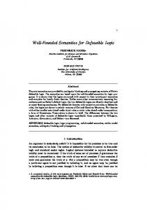
Figure 2: Rule Persistence. A persistent rule r enacted at time t 0 and in force at t 000 carries over from the legal system LS(t 0 ) (the set of norms in vigor at time t 0 ) to the legal system LS(t 00 ), where it is still in force at t 000 .
t
+∂ p a
t0
Figure 3: Causal Conclusion Persistence. A conclusion is causal if it persists from a legal system LS(t 0 ) to a legal system LS(t 00 ) even if the rules used to derive it are no longer effective in LS(t 00 ).
where 1. if p is persistent, t p0 ≤ t∼p ≤ t p , otherwise t p0 = t∼p = t p ;
To illustrate these ideas consider the following theory: r : a10 ⇒ b(20,pers) : 10@(1,trans) s : b30 ⇒ c(30,pers) : 15@(1, pers)
2. ts0 ≤ tv , if s is persistent, otherwise ts = ts0 = tv ; 3. td ≤ ts0 , if s is persistent, otherwise ts = ts0 = td ; 4. if conclusions are persistent over derivations (i.e., +∂td0 @tr p pt implies +∂td @tr p pt where td0 < td ), then, td0 ≤ td00 ≤ td ; 5. if conclusions are persistent over repositories, then tr0 ≤ tr00 ≤ tr . The proof conditions given above produce classes of variants of temporalised defeasible logic, according to conditions on the temporal parameters. In particular it is possible to define variants capturing different types of persistence. Of particular relevance to the application in legimatics, and in particular to legal drafting, consolidation and norm modifications we mention rule persistence and causal conclusion persistence. Generally once a norm has been introduced in a normative system, or better in a specific legal system of the normative system, the norm continues to be in the normative system unless it is explicitly removed (see Section 5 for some possible types of removal). This means that the norm must be included in all legal systems succeeding the legal system in which it has been first introduced (see Figure 2 for a graphical representation of this phenomenon). This effect is achieved by specifying that the derivation of rules is persistent over repositories. On the other hand, if we can prove a conclusion with respect to a specific legal system in some cases we have to propagate it to successive legal systems. In particular this is the case when we have causal conclusions. This was the option we explored in [7]. However, for some type of norm modifications, namely annulment (see Section 5 for a more detailed analysis of this), we have to block the persistence of conclusion over repositories when the reasons for deriving a conclusion are no longer in the legal system. See Figure 3 for a graphical representation of causal conclusion persistence. This effect depends whether derivations of conclusions are persistent over repositories, and it is in function of the particular type of modification we want to implement.
Since r is marked as transient, the rule can be used only in repository 1, while s can be used in all repositories after repository 1.2 Given a10 @1 we can first derive +∂ 10 : 1 b(20,pers) . Since b is persistent we have +∂ 10@1 b20 . Notice the the second rule cannot be applicable, since its validity time is 15. Thus, to apply it we have to assume that derivations are persistent within a repository. If this is the case then we obtain +∂ 15 : 1 b20 , which then makes rule s applicable, and from which we get +∂ 15 : 1 c30 . If we have that conclusions are persistent across repositories, then we can conclude +∂ 15 : 2 c3 0. Notice that we can conclude +∂ 15@2 c30 even if the reasons for deriving it (i.e., rule r) do not persist across repositories.
5.
NORM MODIFICATIONS IN TDL
In this section we consider four kinds of modifications: substitution (which replaces some textual components of a provision with other textual components, or a provision with another provision), derogation (the derogating provision limits the effects of the derogated provision), annulment (which cancels ex tunc a provision and prevents it to produce any normative effect), and abrogation (which cancels a provision but does not cancel the effects that were obtained before the modification). Notice that other types of textual or temporal modifications can be added to our framework following the same rationale adopted below. In TDL, the application of a norm-modifying provision changing a rule r is represented by deriving a set MOD of rules that change the status, or even single parts, of r. This typically happens via the application of one or more meta-rules that lead to obtain the rules in MOD. Notice, however, that it could in theory happen that the rules in MOD exist in a certain repository at tr independently of the application of any meta-rules and that they start to be in force at a time tv0 such that tv0 > tr . Suppose that r comes into existence in a 2 To make the example more clear we have used two different scales for the derivation time and the repository time. Anyway in legal reasoning these will be on the same time scale.
+∂ a r
t0 t 0 tv
t0
+∂ a r
t0 t 00
t 0 tv
+∂ a r
t0 ta
t 00
LS(t 0 )
LS(t 00 )
r : tv @t 0
abrog(r : tv ) : ta @t 00
t0
t 00
Figure 4: Abrogation. In LS(t 0 ) rule r is applied and produces a persistent effect a. The effect carries over by persistence to the legal system LS(t 00 ) even if the rule r is no longer in force to produce the effect.
t 0 tv
t0
r
t0 t 00
t 0 tv
ta
t 00
LS(t 0 )
LS(t 00 )
r : tv @t 0
annul(r : tv ) : ta @t 00
t0
t 00
Figure 5: Annulment. In LS(t 0 ) rule r is applied and produce a persistent effect a. Since the rule is annulled in LS(t 00 ), the effect of a must be undone as well.
Annulment and Abrogation repository at tr0 , tv0 > tr0 > tr , and it gets in force at tv , tv0 > tv > tr . If we admit persistency of rules within and across repositories, then the rules of MOD, if derivable by persistency, will occur in the repository at tv0 and in force at that time. Thus, at tv0 the rules of MOD will affect r without the use of any meta-rule.3 Finally, notice in many but not in all cases (as we will see, derogation is an exception), modifications imply that MOD should at least include a new version of r, namely, that a rule, labelled by r, is in MOD but it is different from the r which was in force before deriving MOD. Let us summarise the reasoning patterns corresponding to the mentioned types of modifications. In the following, ,→∈ {→, ⇒ , ;}.
Substitution Preconditions: +∂td @tr r : (A ,→ C) : tv ; Derived rules MOD: +∂td0 @tr0 r : (A0 ,→ C0 ) : tv0 ; Constraints: (1) A0 6= A or C0 6= C, and (2) tr0 ≥ tr and tv0 6= tv , and (3) −∆td @tr r : (A ,→ C) : tv .
Derogation Preconditions: +∂td @tr r : (A ⇒ C) : tv ; Derived rules MOD: +∂td0 @tr0 r0 : (A0 ⇒ C0 ) : tv0 , +∂td0 @tr0 r00 : (A0 ; ∼C) : tv0 Constraints: (1) A ⊂ A0 and C0 6= C, and (2) tr0 ≥ tr and tv0 6= tv , and (3) −∆td @tr r : (A ⇒ C) : tv . 3 One may consider this case as pathological, as it does not properly correspond to a modification. If so, the following reasoning patterns should explicitly mention what meta-rules are used to derive MOD. The time parameters of the elements of MOD are taken from when the meta-rules are applied.
Preconditions: +∂td @tr r : (A ,→ C) : tv ; Derived rules MOD: +∂td0 @tr0 (r : ⊥) : tv0 ; Constraints: (1) tr0 ≥ tr and tv0 6= tv , and (2) −∆td @tr r : (A ,→ C) : tv . Some comments. The basic assumptions for all cases are that a modification can be applied to r only if r is modifiable and it exists. The first assumption is captured by the last constraint in each case. Let us consider rule existence. Minimally, the existence of rule r is a notion relative to repositories, thus the modification should take place in a subsequent or in the same temporal repository in which r exists. An additional constraint, which has not been mentioned here, is that the modification (i.e., typically, meta-rules) should be in force at a time subsequent to the time when r is in force. This requirement, which is adopted in many cases in legal systems, states in fact that we cannot modify a normative provision which is not yet in force. But this is not general necessary, as we can, at least logically, imagine a situation in which a normative provision r is issued at t but will start to be in force only from t + n. In the time span from t to t + n an authority could change r even if it is not yet in force. Consider, for example, a reform of pension system made in 2007 stating that 60 years people can no longer retire: r : (60YearsOld : 2009 ⇒ ¬PermittedRetire : 2009) : 2009@2007 The norm will be in force in 2009, immediately applicable and effective. The postponement is made to enable people to assess their personal situation and decide whether it is more convenient to retire before 2009 (but with a lower pension income) or accept to wait some more years but earning a higher pension income. Suppose that the new government deliberates in 2008 to modify this reform of 2007 and to remove r. This is indeed possible, even if r is not yet in force. Substitution is simply a modification that changes, partially or entirely, the antecedent or the consequent (or both) of a normative provision r. Derogation can be applied only to defeasible rules: if applied to r, it permits to introduce an exception r0 of r; in this case, the derivation of the exception r0 is drawn together with inferring a
Modifications annul(r : tv ) : ta @t subst(r : tv ) : ta0 @t 0 abrog(r : tv ) : ta @t subst(r : tv ) : ta0 @t 0 annul(r : tv ) : ta @t or derog(r : tv ) : ta0 @t 0 abrog(r : tv ) : ta @t or derog(r : tv ) : ta0 @t 0 subst(r : tv ) : ta @t derog(r : tv ) : ta0 @t 0
Conditions ta = ta0 and t = t 0 ta = ta0 and t = t 0 ta = ta0 and t = t 0 ta = ta0 and t = t 0 ta = ta0 and t = t 0 and A(r0 : tv0 )) ∩ A(r : tv ) 6= A(r : tv ) or C(r00 : tv0 )) 6= ∼C(r : tv )
Table 1: Conflicts defeater r00 that blocks the derivation of the direct effect of r when r0 is applicable. Abrogation and annulment of r have basically the same structure: what makes the former different from the latter is the treatment of the effects of the modified rule. As we mentioned, annulment cancels all effects of r, whereas abrogation does not. Annulment is thus obtained by blocking persistency of derivations across repositories. In other words, the conclusions of the annuled rule will only be derived in the repository in which the modification does not occur (see Section 4.2 and Pictures 4 and 5). With this said, we have now to see when norm modifications can be in conflict. Table 1 summarises the basic conflicts between the norm modifications we have considered. To save space, we refer to previous inference patterns when we need to specify rules r0 and r00 for derogation: r0 is the rule which corresponds to the exception of r, while r00 is the defeater that blocks the conclusion of r in the exceptional case (see above). Notice that in all cases a conflict obtains only if the conflicting modifications apply to the same time instant and in the same repository. Annulment and abrogation of r are incompatible with any substitution in r (first two rows from top). A similar intuition holds for the two subsequent rows: it is impossible to derogate to r if this rule is dropped from the system. Finally, the cases in the last row from the bottom state that a substitution in r is incompatible with a derogation if at least one literal used in r0 or r00 to derogate to r is replaced in r0 or r00 .
6.
CONCLUSIONS AND RELATED WORK
In this paper we extended the logic presented in [7] to capture different temporal aspects of the norm-modification process. This extension increases the expressive power of the logic and it allows us to represent meta-norms describing norm-modifications by referring to a variety of possible time-lines through which conclusions, rules and derivations can persist over time. We outlined the inferential mechanism needed to deal with the derivation of rules and literals. In particular, for each proof condition we identified several temporal constraints that permit to allow for, or block, persistency with respect to specific time-lines. This virtually leads to define different variants of TDL according to whether a condition is adopted or not. Then we described some issues related to norm modifications and versioning and we illustrated the techniques with some relevant norm modifications such as annulment, abrogation, substitution and derogation. We showed that the temporal formalism introduced here is able to deal with complex scenarios such as retroactivity and time-forking. In particular, we solved the problem of how legal effects of ex-tunc modifications, such as annulment, can be blocked after the modification applied. The idea we suggested is to block persistency of derivations across repositories. In other words, the conclusions of the annuled rule will only be derived in the repository in which the modification does not occur. The proposed methodology illustrates the possibilities of the for-
malism and we intend to apply it the the logical analysis of a larger corpus of norm-modifications. Typically there are two mainstream approaches to reasoning with and about time. A point based approach, as in the present paper, and an interval based approach [1]. Notice that that the current approach is able to deal with constituents holding in an interval of time, thus an expression ⇒ a[t1 ,t2 ] meaning that a holds between t1 and t2 can just be seen as a shorthand of the pair of rules ⇒ a(t1 ,pers) and ; ¬a(t2 ,trans) . Currently it is not clear what benefits would result from an interval based temporalised defeasible logic for the intended application. Anyway we would like to point out that interval and duration based temporal defeasible logic have been developed [3, 9]. [9] focuses on duration and periodicity and relationships with various forms of causality. [3] proposed a sophisticated interaction of defeasible reasoning and standard temporal reasoning (i.e., mutual relationships of intervals and constraints on the combination of intervals). In both cases it is not clear whether the techniques employed by the papers are relevant to the application to norm modifications, and both papers consider only a single temporal dimension, and do not have meta-rules.
7.
REFERENCES
[1] J.F Allen. Towards a general theory of action and time. Artificial Intelligence, 23:123–154, 1984. [2] Grigoris Antoniou, David Billington, Guido Governatori, and Michael J. Maher. Representation results for defeasible logic. ACM Transactions on Computational Logic, 2(2):255–287, 2001. [3] Juan Carlos Augusto and Guillermo Ricardo Simari. Temporal defeasible reasoning. Knowledge and Information Systems, 3(3):287–318, 2001. [4] Nick Bassiliades, Grigoris Antoniou, and Ioannis Vlahavas. DR-DEVICE: A defeasible logic system for the Semantic Web. In H.J. Ohlbach and S. Schaffert, editors, 2nd Workshop on Principles and Practice of Semantic Web Reasoning, 2004. [5] Guido Governatori, Michael J. Maher, David Billington, and Grigoris Antoniou. Argumentation semantics for defeasible logics. Journal of Logic and Computation, 14(5):675–702, 2004. [6] Guido Governatori, Vineet Padmanabhan, and Antonino Rotolo. Rule-based agents in temporalised defeasible logic. In Qiang Yang and Geoff Webb, editors, Ninth Pacific Rim International Conference on Artificial Intelligence, number 4099 in LNAI, pages 31–40, Berlin, 7–11 August 2006. Springer. [7] Guido Governatori, Monica Palmirani, R´egis Riveret, Antonino Rotolo, and Giovanni Sartor. Norm modifications in defeasible logic. In Marie-Francine Moens and Peter Spyns, editors, Legal Knowledge and Information Systems,
[8]
[9]
[10] [11]
[12]
[13]
[14] [15]
[16] [17]
number 134 in Frontieres in Artificial Intelligence and Applications, pages 13–22. IOS Press, Amsterdam, 2005. Guido Governatori, Antonino Rotolo, and Giovanni Sartor. Temporalised normative positions in defeasible logic. In Anne Gardner, editor, 10th International Conference on Artificial Intelligence and Law (ICAIL05), pages 25–34. ACM Press, June 6–11 2005. Guido Governatori and Paolo Terenziani. Temporal extension of defeasible logic. In Hans W. Guesgen, G´erard Ligozat, and Rita V. Rodriguez, editors, Proceedings of the IJCAI’07 Workshop on Spatial And Temporal Reasoning, page ? IJCAI, 6 January 2007. Riccardo Guastini. Teoria e dogmatica delle fonti. Giuffr´e, Milan, 1998. Michael J. Maher. Propositional defeasible logic has linear complexity. Theory and Practice of Logic Programming, (6):691–711, 2001. Donald Nute. Defeasible reasoning. In Proceedings of 20th Hawaii International Conference on System Science, pages 470–477. IEEE press, 1987. Donald Nute. Defeasible logic. In Dov Gabbay, Christopher Hogger, and John Robinson, editors, Handbook of Logic in Artificial Intelligence and Logic Programming, volume 3, pages 353–395. Oxford University Press, 1993. R. Pagano. L’arte di legiferare. Giuffr´e, Milan, 2001. Monica Palmirani and Raffaella Brighi. Time model for managing the dynamic of normative system. In Proceedings of EGOV 2006, pages 207–218, Berlin, 2006. Springer. Giovanni Sartor. Legal Reasoning. Springer, Dordrecht, 2005. Bart Verheij. Virtual Arguments. On the Design of Argument Assistants for Lawyers and Other Arguers. T.M.C. Asser Press, The Hague, 2005.