Variational Bayesian Inference for the Latent Position Cluster Model Michael Salter-Townshend School of Mathematical Sciences University College Dublin Ireland
[email protected]
Thomas Brendan Murphy School of Mathematical Sciences University College Dublin Ireland
[email protected]
Abstract Many recent approaches to modeling social networks have focussed on embedding the actors in a latent “social space”. Links are more likely for actors that are close in social space than for actors that are distant in social space. In particular, the Latent Position Cluster Model (LPCM) [1] allows for explicit modelling of the clustering that is exhibited in many network datasets. However, inference for the LPCM model via MCMC is cumbersome and scaling of this model to large or even medium size networks with many interacting nodes is a challenge. Variational Bayesian methods offer one solution to this problem. An approximate, closed form posterior is formed, with unknown variational parameters. These parameters are tuned to minimize the Kullback-Leibler divergence between the approximate variational posterior and the true posterior, which known only up to proportionality. The variational Bayesian approach is shown to give a computationally efficient way of fitting the LPCM. The approach is demonstrated on a number of data sets and it is shown to give a good fit.
1 The Latent Position Cluster Model Handcock et al. [1] developed the Latent Position Cluster Model (LPCM) for social network data. The model involves locating each actor in a latent social space such that actors who are close in social space have a higher probability to form links than those distant in the social space. This model extended the Latent Space Model (LSM) [2] by incorporating a Gaussian mixture model structure for the latent positions of actors in social space, to accommodate the clustering of nodes in the network. Therefore clusters are included explicitly in the model rather that found by post-hoc analysis of the network model. A strength of the latent social space model is that it automatically represents link transitivity. We develop a variational Bayesian inference procedure for approximating the posterior distribution of the parameters in the LPCM. This approach provides computational tools to facilitate the application of the LPCM to larger networks than is currently possible using the existing MCMC methodology for model fitting. In the LPCM, a binary interactions data matrix Y is modelled using logistic regression in which the probability of a link between two nodes depends on the distance between the nodes in the latent space: log-odds(yi,j = 1|zi , zj , β) = β − |zi − zj | (1) where β is an intercept parameter and |zi − zj | is the Euclidean distance between the latent positions of nodes i and j. In addition, the links are assumed to be independent conditional on the latent positions of the actors in the latent space. 1
To represent the clustering, the latent positions Z are modeled as coming from a mixture of G multivariate normal distributions: zi ∼
G ∑
λg MVNd (µg , σg2 Id )
(2)
g=1
where λg is the probability that actor i belongs to the g th group, so that λg ≥ 0, {g = 1, . . . G} and ∑G g=1 λg = 1, and Id is the d × d identity matrix. The parameters β, λ, σ and µ are also given prior distributions. The full set of hierarchical priors is:
zi
∼
G ∑
λg MVNd (µg , σg2 Id )
(3)
g=1
λ ∼ Dirichlet(ν)
(4)
∼ Normal(ξ, ψ )
(5)
µg
∼ MVNd (0, ω Id )
(6)
σg2
∼
(7)
β
2
2
σ02 Inv
−
χ2α
The posterior is then given by: p
= p(Z, λ, β, µ, σ 2 |Y ) = Cp(Y |β, Z)p(Z|λ, µ, σ 2 Id ) p(λ|ν)p(β|ξ, ψ 2 )p(µ|0, ω 2 Id )p(σ 2 |σ02 , α)
The constant C is unknown so that the posterior is only known up to proportionality. ξ, ψ and ω 2 are fixed hyperparameters. 1.1
(8) 2
, ν, σ02 , α
MCMC Based Inference
To facilitate MCMC based inference, latent indicator vectors K1 , K2 , . . . , KN are introduced; there is one such vector per actor, with each element of the vector being zero, except for a one in the entry corresponding to the group to which that actor belongs. The form of the latent vectors K therefore Ki ∼ Multinomial(1, λ) for i = 1, 2, . . . , N . In this augmented setup, sampled positions Z are therefore “hard clustered” to the groups. Samples of {Z, K, λ, β, µ, σ} are drawn from the posterior from Equation (8) using Markov Chain Monte Carlo; for details see [1, 3]. This approach to fitting the LPCM is computationally very expensive. Using the R package latentnet [3], for even the very small example of Sampson’s monks data (18 nodes; see Section 3.2) the package requires over a minute to generate just 4,000 samples from the posterior. Convergence is difficult to assess and mixing is difficult to optimise as the model involves many strongly dependent terms. The computational overhead scales as O(N 2 ) so that MCMC based inference on large networks is extremely expensive in terms of computation. Although latentnet works well with small networks, modelling networks with more than a couple of hundred nodes is impractical.
2
Variational Bayesian Inference
We loosely follow the method of [4] who use a variational approximation to fit a mixed-membership stochastic blockmodel; however we find a variational approximation for the LPCM. In fact, this work is prompted in that paper when the authors state “It would be interesting to develop a variational algorithm for the latent space models”. A closed form distribution q(Z, λ, β, µ, σ 2 |Y ) is formed, with unknown variational parameters. These parameters are then optimised by minimization of the Kullback-Leibler divergence from q to the true posterior p given in Equation (8), which is known only up to proportionality. 2
This minimization is achieved via an iterative search algorithm that is similar to the ExpectationMaximisation (EM) algorithm. The computational overhead required to find the optimal variational posterior is far less than for sampling based methods like MCMC. This variational posterior is a closed-form approximation to the true posterior and can be used for subsequent inference for model parameters. The Kullback-Leibler divergence (KL) is defined by KL = Eq [log(q)] − Eq [log(p)].
(9)
Minimization of KL does not require knowledge of the normalization constant of the true posterior because Eq [log(p/C)] = Eq [log(p)] − log C for all C > 0. 2.1 Specification of the Variational Model Using the restricted or quasi variational Bayesian approach, we propose a variational posterior in the same form as the prior, but with unknown variational parameters. We distinguish the variational parameters with by putting a tilde over them. The variational posterior is of the form: q
= q(Z, λ, β, µ, σ 2 |Y ) ˜ ˜ ψ˜2 ) ˜ σ = q(Z|Z, ˜ 2 )q(K|λ)q(λ|˜ ν )q(β|ξ, q(µ|˜ η, ω ˜ 2 )q(σ 2 |˜ α).
(10)
Note that the above form of q is fully factorized and this is also known as a mean-field approximation. Such a model allows for analytical integrations to be performed in computing the expectations required when evaluating the Kullback-Leibler divergence in Equation (9). A more obvious variational posterior would comprise only distributions on the latent positions Z, the cluster membership indicators K and the intercept term β. However, we wish to capture as much of the detail in the original MCMC posterior as possible, hence the need for the inclusion of the other terms. Without these, our variational posterior would not inform us on the size and location of the groups/clusters. Equation (10) represents a fully Bayesian variational posterior. As a general result, the factorised variational posterior gives an approximation to the true posterior that has support that is too compact [5, Section 10.1.2]. 2.2
Updating the Variational Parameters
The variational parameters are tuned to minimise the Kullback-Leibler divergence from q to p. The KL divergence is computed and then differentiated with respect to each of the variational parameters. An initial configuration of the variational parameters is chosen (see Section 4.1). The algorithm then iterates around each set of variational parameters in turn. Within each set the algorithm runs randomly through the sequence of variational parameters and minimises the Kullback-Leibler divergence. In each case, all other variational parameters are held fixed and the Kullback-Leibler divergence is optimised with respect to the variational parameter being updated. Convergence to a steady state (local minimum on the KL surface) is reached after a number of iterations, depending on the convergence criterion used. ˜ η˜, ω For the variational parameters λ, ˜ 2 , a closed form update equation was found. For all other variational parameters, numerical optimisation was required. A fast bracketing-and-bisection algorithm was used to find the minimum KL divergence in each case. The first derivative of the KL divergence as a function of each variational parameter was computed and the value of the parameter for which this function is zero gives the updated estimate. However, the bracketing and bisection algorithm ˜ therefore a slower, was found to be unstable for the latent positions Z˜ and the intercept parameter ξ; but more robust, quasi-Newton method was employed. 2.2.1
Algorithm
The variational inference algorithm proceeds as outlined below. The analytical updates are available when the partial derivative of Kullback-Leibler divergence w.r.t the term being updated as set equal to zero is re-expressible with the updated term only on one side. Otherwise, a more complicated 3
equation with multiple instances of the updated term is found and numerical optimisation must be used. In cases where the term being updated is a vector or a matrix the entries are cycled through in a random order. ˜ i,g , ν˜g , ξ, ˜ ψ˜2 , η˜g , ω 1. initialize z˜i , σ ˜i2 , λ ˜ g2 , α ˜ g for all i, g. 2. repeat in a randomized order 3. update ξ˜ via quasi-Newton. 4. update ψ˜2 via bisection. 5. update Z˜ via quasi-Newton. 6. update η˜ 2 via analytical function. 7. update σ ˜ via bisection. ˜ via analytical function. 8. update λ 9. update ω ˜ 2 via analytical function. 10. update α ˜ via bisection. 11. update ν˜ via bisection. 12. until convergence 2.3
Expectation of the Log-Likelihood
A tractable approximation of the expected log-likelihood is derived by using a first order Taylor expansion three times to get: Eq [log(p(Y |β, Z))]
=
N ∑ N ∑ i
≃
N ∑ N ∑ i
=
yi,j Eq [β − |zi − zj |] − log (1 + Eq [exp(β − |zi − zj |)])
j
N ∑ N ∑ i
yi,j Eq [β − |zi − zj |] − Eq [log (1 + exp(β − |zi − zj |))]
j
( )1 yi,j (ξ˜ − |˜ zi − z˜j |2 + d(˜ σi2 + σ ˜j2 ) 2 )
j
( ) − log 1 + Eq(β) [exp(β)]Eq(z) [exp(−|zi − zj |)] ≃
N ∑ N ∑ i
)1 ( ˜j2 ) 2 ) yi,j (ξ˜ − |˜ zi − z˜j |2 + d(˜ σi2 + σ
j
(
ψ˜2 − log 1 + exp(ξ˜ + + Eq(z) [−|zi − zj |]) 2 ≃
N ∑ N ∑ i
)
( )1 ˜j2 ) 2 ) yi,j (ξ˜ − |˜ zi − z˜j |2 + d(˜ σi2 + σ
j
(
)1 ) ψ˜2 ( − log 1 + exp(ξ˜ + − |˜ zi − z˜j |2 +d(˜ σi2 + σ ˜j2 ) 2 ) 2
3 3.1
(11)
Examples Simulated Data
Application of the variational inference method was applied to simulated data composed of 3 groups in a 2-D social space. The binary interactions matrix Y was simulated in the following manner: β = 1.0 [ ] [ ] µ1 −2 2 0 −2 µ = = µ2 = µ3 2 2 2 2 σ2 = = [σ12 , σ∑ 2 , σ3 ] = [0.1, ∑ 0.05,20.3] zi ∼ MVN2 ( Kig µg , Kig σg I2 ) Yi,j ∼ Bernoulli(logit−1 (β − |zi − zj |)) 4
for i, j = 1, . . . , N and with K constructed such that it assigns (approximately) 25% of the actors each to groups 1 and 2 and the rest to group 3; this corresponds to setting λ = [λ1 , λ2 , λ3 ] = [0.25, 0.25, 0.50]. The advantage of using simulated data is that the ground truth is known; however we are simulating from the exact model that we are then fitting to the data. We can compare results obtained using our variational method to the values used in generating the simulated data. Over repeated experiments, our method performs very well at recovering the data generating mechanism. Again, the caveat is that we are fitting the exact model that was used to generate the data. We also use this dataset to explore the impact of the initialization procedure on performance in Section 4.1. 3.2
Sampson’s Monks Data
The much analysed Sampson’s monks dataset [6] serves as a familiar testing ground for our inference methodology. Eighteen monks in a cloister were each asked sociometric questions. As per [1], we focus on the relationship “liking”. The data are an 18 × 18 matrix with ones corresponding to a links and zeros corresponding to non-links. We compare our variational results with the MCMC result obtained via latentnet. Figure 1 shows the default posterior plot generated using latentnet along with our variational equivalent. The plot depicts the posterior modal positions with a pie chart for each monk depicting the posterior probability of that monk belonging to each of the three groups. The links between monks are depicted with grey arrows. The group standard deviations in the latent space are indicated with a coloured circle, centred on the group mean posterior position, which is indicated with a coloured cross. It is clear that our approximate method has captured the essential structure of the MCMC posterior. A posteriori, the monks are grouped into the same clusters and the latent positions have a similar pattern in the social space. The key differences to note are that the variational inference clusters are not as far apart and that the membership probability vectors are closer to a hard clustering. In fact, these two variations from the MCMC result appear contradictory and are possible due to the factorised structure of the variational approximation. Latentnet Solution
Variational−Bayes Solution
4
2
6
3
samplike ~ latent(d = 2, G = 3)
2
1
+
Z2
0
0
−2
−1
Z2
+ +
−6
−3
−4
−2
+
−4
−2
0
2
4
−5
Z1
0
5 Z1
Figure 1: Posterior Positions of Sampson’s monks dataset, using MCMC and the Variational method. The latter is rotated via a Procrustes transformation to facilitate comparison with the former. The initialization method used in the variational algorithm was the Fruchterman-Reingold method (see Section 4.1). 3.3
An Egocentric Facebook Network
We examine an egocentric network in which the actors are members of the social networking website Facebook. The egocentric network for a single actor (an author of this paper) comprises the 81 “Facebook friends” with which the actor is linked. We remove this central actor and explore 5
the structure of the links between the remaining nodes. The nodes cluster nicely into several social groups which have a clear intuitive interpretation. The six groups are: school (black), college (green), former housemates (dark blue), partners friends (light blue), family (red) and Norwegians (purple). The groups interact a varying amount with all groups except school interacting heavily with a central figure (the author’s partner). The Norwegians interact only with each other and this central actor. A single actor (author’s brother) joins family and school, with school otherwise disconnected from the rest. The data was generated using a Facebook application that is available at http://apps.facebook.com/mynet_phaseone/ MCMC and variational results are compared in Figure 2. Latentnet Solution
Variational−Bayes Solution
10
20
Y ~ latent(G = 6, d = 2)
+
+
0
0
+
5
+
Z2
Z2
5
10
15
+
−5
−5
+
−10
+
−10
−5
0
5
10
−15
Z1
−10
−5
0
5
10
15
Z1
Figure 2: Posterior Positions of a Facebook dataset, using MCMC and the Variational method. The latter is rotated via a Procrustes transformation to facilitate comparison with the former. MCMC inference took approximately 28 minutes; the variational algorithm converged in just over 2.5 minutes.
4 4.1
Assessing the Variational Approximation Impact of Initialization Method
Good initialization of the variational parameters is crucial to the method because the KullbackLeibler divergence to the true posterior may contain many local minima. Starting the algorithm at different values for the variational parameters and updating (Section 2.2) demonstrates that the algorithm can converge to different minima given different starting values. There are two desirable criteria for the initial configuration: the initialization procedure should be fast and the resultant configuration should be as close as possible to the global minimum; this should minimise the chances of the iterative updates becoming stuck in a local minimum. We experimented with four options for the initial configuration: (1) The ground truth, when available (2) Estimating positions via multidimensional scaling of the interactions matrix, then clustering using mclust [7]. (3) Positions via the Fruchterman-Reingold [8] method, then mclust clustering (4) Positions and clustering via output from latentnet. Method (1) is available only when exploring simulated data (see Section 3.1). The main advantage of method (2) is that there is no randomness involved; i.e. the method delivers the same initial configuration under multiple re-runs. Results for the latent positions are similar to the latentnet MCMC posterior. Method (3) initializes the positions in a visually pleasing configuration. Method (4) serves only for comparison with the existing MCMC inference and is impractical; if MCMC inference has already been performed then our variational approximation has little extra to offer. The use of the MCMC modal output to initialize our variational method reveals that our method is highly susceptible to convergence to a local minimum. When the monks example was initialized 6
Table 1: Means and standard deviations for the expected log-likelihood under multiple simulations given various initialization techniques. Ground truth MDS FR mean -10.06 -20.87 -11.73 sd 0.58 4.44 0.86
Table 2: The multi-run parameter mean and standard deviation for mean-squared-errors given various initialization techniques. Ground truth is starting with the true values used to generate the data, MDS is multidimensional scaling with clustering and FR is Fruchterman-Reingold with clustering. Ground truth MDS FR MSE MSE MSE mean sd mean sd mean sd Z 0.1159 6.198 × 10⁻² 1.664 0.567 1.496 0.748 β 4.690 × 10⁻² 8.642 × 10⁻³ 0.335 0.136 6.672 × 10⁻² 1.779 × 10⁻² µ 7.545 × 10⁻² 0.344 2.478 1.966 0.402 0.346 2 σ 1.161 × 10⁻² 3.894 × 10⁻⁶ 1.168 × 10⁻² 1.369 × 10⁻⁴ 1.162 × 10⁻² 2.584 × 10⁻⁵ λ 4.025 × 10⁻⁶ 7.921 × 10⁻⁶ 7.282 × 10⁻⁴ 1.741 × 10⁻³ 3.846 × 10⁻⁴ 1.378 × 10⁻³
using the latentnet MCMC posterior, the variational result was closer to the MCMC result than that depicted in Figure 1. We performed re-runs of the simulated data example with 3 groups and 20 actors and computed the approximate expected log-likelihood E[LL] (Equation (11)) for the first three initialization options (ground truth, multidimensional scaling (MDS), and Fruchterman-Reingold (FR)). Crude initialization using completely random values for the variational parameters invariably led to convergence to markedly different configurations, with far lower E[LL] values. We compare the more useful initialization procedures with initialization using the ground truth. The mean and standard deviation of the expected log-likelihoods over 100 runs using the various initialization methods is given in Table 1. The mean and standard deviations for the mean squared errors of the latent positions Z and model parameters (β, µ, σ 2 , λ) are given in Table 2. In our experience with the various initialization methods, the Fruchterman-Reingold method leads to good parameter estimates and prediction of both links and non-links (see Section 4.3). The multidimensional scaling method leads to a small improvement in predicting the non-links and a loss in predictive performance for the links. 4.2
Scalability and Speed
As with MCMC, our algorithm scales as O(N 2 ). However, the variational method is far quicker than MCMC, involving fewer computations as it is not sampling based. Convergence of the variational algorithm for the monks dataset took approximately 2 seconds on a machine that runs the latentnet MCMC version with 4000 iterations (the default number) in 64 seconds. For the Facebook data, the times were 156 seconds and 1697 seconds respectively. For a simulated dataset involving 300 nodes and 9 groups, our algorithm performed 100 variational update iterations in around 700 seconds on a standard PC. Using the criterion that a parameter is deemed to have converged to an optimal value when the change in updated parameters falls below 10−10 , the variational algorithm converged in 54 iterations. The code is written in C and called from R. The MCMC version of latentnet was impractical for this size of network. 4.3
Predictive Probability of a Link
Model fit was assessed by splitting the data into links and non-links and plotting the posterior predictive probability of a link between actors for both the links and non-links. This provided an intuitive technique for assessing the model fit. If the zeros in the interactions data matrix Y are associated with posterior predictive probabilities that are distributed close to zero then the model is doing a 7
good job of modelling the non-links. The converse is also true for the links. Figure 3 shows the posterior predictive fits to the Facebook dataset. This figure, along with Figures 1 and 2, suggest that the variational method returns results that are closer to the MCMC posterior for higher N .
MCMC Predict Fit
Variational Predict Fit
4
Density
6
8
Yij = 0 Yij = 1
0
2
4 0
2
Density
6
8
Yij = 0 Yij = 1
0.0
0.2
0.4
0.6
0.8
1.0
0.0
Predicted probability of a link
0.2
0.4
0.6
0.8
1.0
Predicted probability of a link
Figure 3: Smoothed density plots of the posterior predictive probability of a link, for the Facebook dataset. The left side plot was obtained using MCMC and the right side plot using the variational method. The posterior predictive probabilities are split according to whether the data shows a link (red density) or not (black density). The faster variational method performs almost identically to the MCMC method.
5
Discussion
We have presented a variational inference routine to tackle the computational problems associated with Bayesian analysis of social networks using the Latent Position Cluster Model (LPCM). Although our method is approximate but it captures the essentials of the current standard methodology with much less computational burden. However, our algorithm converges in a short number of fast iterations compared to sampling based methods, so we can analyse larger graphs than are possible under the MCMC method. Our contribution is to the inference methodology for the LPCM rather than development of a new model for network data. Therefore, we have only presented results comparing our variational method to MCMC. Also for this reason - and for brevity - we do not present model choice diagnostics. Although we have only discussed our method in terms of binary link data, our method extends readily to other network data types. We experimented with various initialization techniques for the variational parameters. Good initial values are crucial as the method is prone to convergence to a local minimum of the Kullback-Leibler divergence. In a simulation study, we compare two competing initialization methods with each other and with initialization to the ground truth values used to generate the data. Based on the meansquared error diagnostics in Table (2) We find that the Fruchterman-Reingold method performs better than the multidimensional scaling technique. The variational inference methodology can be extended to account for other network link types, the inclusion of covariate data on the nodes and richer models, such as those including sender and receiver effects. We have stated that our method is prone to convergence to local minima of the Kullback-Leibler divergence; a test for convergence to the global minimum is not straightforward but would present a significant advancement of the methodology. More sophisticated and computationally efficient initialization methods would be beneficial. Parallelization of the C code written to implement our method may increase the practical applicability of our method to very large networks. We envisage building a publicly available R package to perform the variational inference method outlined herein. 8
References [1] M. S. Handcock, A. E. Raftery, and Tantrum J. M. Model-based clustering for social networks. Journal of the Royal Statistical Society: Series A, 170(2):1–22, 2007. [2] P. Hoff, A. E. Raftery, and M. S. Handcock. Latent space approaches to social network analysis. Journal of the American Statistical Association, 97:1090–1098, 2002. [3] P. N. Krivitsky and M. S. Handcock. Fitting latent cluster models for social networks with latentnet. Journal of Statistical Software, 24(5), 2008. [4] E. M. Airoldi, D. M. Blei, S. E. Fienberg, and E. P. Xing. Mixed-membership stochastic blockmodels. Journal of Machine Learning Research, 9:1981–2014, 2008. [5] C. M. Bishop. Pattern Recognition and Machine Learning. Springer, 2006. [6] S. F. Sampson. Crisis in a Cloister. PhD thesis, Cornell University, 1969. [7] C. Fraley and A. E. Raftery. Mclust version 3 for R: Normal mixture modeling and model-based clustering. Technical Report, Department of Statistics University of Washington, Seattle, USA, 2007. http://www.stat.washington.edu/mclust. [8] T. M. J. Fruchterman and E. M. Reingold. Graph drawing by force-directed placement. Software - Practice and Experience, 21(11):1129–1164, 1991.
9