Variational Bayesian inference with Gaussian-mixture ... - Project Euclid

Electronic Journal of Statistics Vol. 8 (2014) 355–389 ISSN: 1935-7524 DOI: 10.1214/14-EJS887

Variational Bayesian inference with Gaussian-mixture approximations O. Zobay Department of Mathematics, University of Bristol, University Walk, Bristol BS8 1TW, United Kingdom∗ Abstract: Variational Bayesian inference with a Gaussian posterior approximation provides an alternative to the more commonly employed factorization approach and enlarges the range of tractable distributions. In this paper, we propose an extension to the Gaussian approach which uses Gaussian mixtures as approximations. A general problem for variational inference with mixtures is posed by the calculation of the entropy term in the Kullback-Leibler distance, which becomes analytically intractable. We deal with this problem by using a simple lower bound for the entropy and imposing restrictions on the form of the Gaussian covariance matrix. In this way, efficient numerical calculations become possible. To illustrate the method, we discuss its application to an isotropic generalized normal target density, a non-Gaussian state space model, and the Bayesian lasso. For heavy-tailed distributions, the examples show that the mixture approach indeed leads to improved approximations in the sense of a reduced Kullback-Leibler distance. From a more practical point of view, mixtures can improve estimates of posterior marginal variances. Furthermore, they provide an initial estimate of posterior skewness which is not possible with single Gaussians. We also discuss general sufficient conditions under which mixtures are guaranteed to provide improvements over single-component approximations. AMS 2000 subject classifications: Primary 62F15; secondary 62E17. Keywords and phrases: Approximation methods, variational inference, normal mixtures, Bayesian lasso, state-space models. Received March 2011.

1. Introduction Recently, the Variational Bayes (VB) method has attracted growing interest as an alternative to Monte-Carlo integration in computational Bayesian inference (for reviews from the perspectives of different fields see, e.g., Opper and Saad (2001), Smidl and Quinn (2005), Bishop (2006), Wainwright and Jordan (2008), Ormerod and Wand (2010)). Together with the ease of application, the increasing popularity of this method is mainly due to the significant increase in computation speed which can be achieved for wide classes of statistical models. However, a serious impediment to an even more widespread use arises from the fact that VB is only approximate and that, in general, it is very difficult to assess ∗ Present address: MRC Institute of Hearing Research, University Park, Nottingham NG7 2RD, UK.

355

356

O. Zobay

the quality of VB calculations without comparing to exact results. A major task for research on variational Bayesian techniques is therefore the development of methodology that allows us to improve VB results in a simple and flexible way. The purpose of the present paper is to contribute to this objective in the context of certain types of Variational Bayes calculations. The basic idea of the VB method consists in approximating a target probability density p, for example a complicated Bayesian posterior, by a simpler one for which one can compute inferences more easily. To this end, one defines a set of functions Q within which one finds the approximation q by minimizing the Kullback-Leibler (KL) distance or relative entropy between the functions in Q and the target p, i.e., Z q′ (1) q = argmin q ′ log . p q′ ∈Q For simplicity, the members of the set Q will be called trial functions in the following. The quality of the approximation crucially depends on the choice of Q. Most applications of the VB method make use of what we will call the factorized or “nonparametric” approach. In this case, Q is chosen as theQset of all completely or partially factorized trial functions, e.g., q(x1:n ) = ni=1 qi (xi ) with x1:n shorthand for the parameter vector (x1 , . . . , xn ), with no restriction on the form of the factors besides normalization (the fully factorized case is also known as mean-field VB). In practice, this approach is then mainly applied to “conjugate-exponential” Bayesian target distributions p, for which the data likelihood is in the exponential family and priors are chosen as conjugate. In this case, the optimized VB factors turn out to belong to the same classes of distributions as the priors, and the minimization problem (1) can be solved efficiently by means of an iteration scheme that updates a finite vector of parameters. This method is attractive as it is simple and often computationally very fast. However, major drawbacks consist in the complete neglect of correlations between variables in different factors, and the restriction to certain types of probability models. Furthermore, it requires substantial effort to find tractable sets of trial functions that improve upon the factorized form. Alternative to this nonparametric approach, one can also choose the trial functions to belong to a prespecified class of distributions1 , typically the multivariate normal family (Opper and Archambeau 2009). The optimization (1) is then with respect to the mean µ and covariance matrix Σ of the Gaussian and has to be carried out using multidimensional numerical minimization procedures such as the conjugate-gradient method. So far this approach has received much less attention than the nonparametric method. This might be attributable, at least in part, to the fact that in general, the size of the covariance matrix, and hence the number of variables to be optimized, grows quadratically with the length n of the parameter vector x1:n (Opper and Archambeau 2009). However, as also pointed out in Opper and Archambeau (2009), the target distribution 1 One can of course also consider the mixed or “semiparametric” case, where some factors within a factorization approach are treated parametrically.

Variational Bayes with Gaussian mixtures

357

p may impose strong constraints on the optimal form of Σ which considerably reduce the number of free parameters. In this way, the problem can be alleviated significantly (alternatively, one can also restrict the form of Σ “by hand”, if a reasonable guess is available). An obvious advantage of the parametric method over the factorization approach lies in the fact that the former is able to describe correlations between variables. Furthermore, it is also applicable to statistical models outside the conjugate-exponential class. However, these advantages come at the cost of restricting the functional form of the marginals. In order to improve the quality of VB results, the use of mixture distributions as trial functions might suggest itself as a natural strategy. A wide variety of probability distributions can efficiently be approximated by mixture distributions, and it is typically straightforward to compute inferences for them. Unfortunately, R for mixtures the analytical calculation of the (differential) entropy S = − q ln q, and thus of the KL distance, is intractable, in general. The solution of the optimization problem (1) therefore becomes more demanding. Jaakkola and Jordan (1998) have derived a variational lower bound for the entropy based on a factorization approach, but on the whole, the study of mixture trial distributions has not received much attention in the literature so far. In the present paper, we consider the use of normal mixture distributions within a parametric VB approach. Our work is thus complementary to the proposal of Jaakkola and Jordan (1998). The computation of the entropy is dealt with by making use of an alternative lower-bound approximation and restricting the choice of covariance matrices for the mixture components. In this way, efficient numerical calculations become feasible. As this treatment is only concerned with the entropy term S in the KL distance, the procedure can be applied whenever the VB problem can be solved for a single-component Gaussian, and it requires an only modestly increased effort. Furthermore, while the method cannot be guaranteed to always lead to an improved solution, we expect it to do so in a large number of cases. In the paper, we discuss the application of this approach to a non-Gaussian state-space model and to the Bayesian lasso as examples of a “realistic” use of the method, and show that it can provide appreciable improvements under appropriate conditions. Note that “improvement” is to be understood in this context as a reduction in KL distance, in agreement with the overall VB strategy. The paper is organized as follows. In Sec. 2 we first discuss some general qualitative considerations regarding the use of mixture distributions in variational Bayesian calculations. We then give a representation of the entropy S in terms of overlap contributions from mixture components, somewhat reminiscent of the inclusion-exclusion formulas of set and probability theory. The mathematical form of this representation motivates a simple lower bound to the mixture entropy S which allows for an approximate calculation of the KL divergence. Section 3 describes the implementation of this framework using mixtures of normal distributions with suitable restrictions on the choice of covariance matrices. In order to illustrate some aspects of the general qualitative behavior of the approach, we discuss a simple model problem with an isotropic target probability

358

O. Zobay

density. Section 4 derives two simple criteria that allow us to check whether a mixture is guaranteed to improve upon a single-component approximation. The criteria are obtained by performing stability analyses of the single-component minimum in the KL divergence with respect to mixture trial functions. In Sec. 5, mixture VB is applied to the non-Gaussian state-space model mentioned above. The posterior distribution of the hidden variables is approximated with singleand multi-component Gaussian trial functions. Comparisons to Markov chain Monte-Carlo results show appreciable improvements in the calculation of the variances, thus justifying the use of mixture trial distributions. We also show that mixtures allow us to approximately calculate posterior skewness, which is not possible with single Gaussians. Section 6 provides an example with realistic data by applying the method to the Bayesian lasso. Finally, Sec. 7 gives a brief summary and some concluding remarks. 2. Variational approximations with mixtures In this section, we first discuss some general aspects of VB approximations with mixture distributions. We then consider the representation of the entropy in terms of overlap contributions of mixture components. This motivates a simple lower-bound approximation of the mixture entropy which forms the basis of the subsequent developments. First of all, however, we return to the general formulation (1) of the VB optimization problem and recall two basic consequences that we will refer to later on. 2.1. General considerations (i) We can think of the optimal VB solution as being determined by a compeR tition betweenR the negative-entropy part S¯ := −S = q ln q and the “energy term” E = − q ln p in the KL divergence. The minimization of the energy E alone would localize q as a Dirac delta function at the global maximum of the target distribution p. However, this contraction is counteracted by the influence of the entropy which tries to spread out the distribution q as much as possible. The actual minimum of the KL distance strikes a balance between these two opposing tendencies. Figure 1 shows a schematic graphical illustration of this principle. The horizontal coordinate of the graph represents a generic measure of the dispersion of the trial functions; for example it could stand for the width of a trial distribution centered at the maximum of p, or it might indicate the distance between two mixture components which are otherwise kept fixed. (ii) The VB approximation q tends to be localized within the support of the target distribution as far as possible, i.e., typically q is small wherever p is, but not necessarily vice Rversa (Minka 2005). This is simply because otherwise the energy term E = − q ln p would impart a huge penalty on the KL divergence. As the trial functions cannot reproduce the shape of the target perfectly, this behavior results in the underestimation of variances as a typical feature of VB


359

KL E

S z ¯ energy E, and KL disFig 1. Schematic showing typical dependence of negative entropy S, tance S¯ + E on some generic coordinate z representing dispersion of trial functions (see text).

approximations. For factorized VB, this problem increases with the strength of correlations between variables in the target (Bishop 2006). We now turn to the discussion of VB approximations with mixture distributions, P i.e., we assume the Pset Q to consist of trial functions of the form q˜ = ki=1 wi q˜i with wi ≥ 0, ki=1 wi = 1. The mixture components q˜i are taken from some prespecified set Q0 of distributions. As schematically illustrated in Fig. 2, we expect there to be two main ways of how mixture distributions can improve the VB approximation. First of all, consider target distributions with multiple well-separated modes [Fig. 2(a)]. A single-component VB solution will typically be localized within one of the pieces of p, whereas an approximation with a mixture distribution may be able to describe the whole target. However, such situations can easily be handled with the help of a straightforward generalization of the one-component approach. Typically, the various parts of p will each give rise to a local minimum of the optimization problem, and the trial functions qi corresponding to these minima will also be well-separated, i.e., have very small overlap. Under this crucial condition of negligible overlap, the qi ’s are readily combined to a global approximation X exp(−Ki )qi (2) q∝ i

of the target. In (2), Ki denotes the KL distance between qi and p. An explanation and further discussion of this relation are given in Zobay (2009). Here we only emphasize that (2) shows how a careful analysis of the local solutions of the VB optimization problem (1) may already lead to efficient improvements of VB approximations in terms of mixtures. In such cases, one does not have to deal with complications arising from calculating the mixture’s entropy. Figure 2(b) shows the second and more interesting way of how mixtures can enhance VB approximations, which we will focus on in the rest of the paper. In

360

(a)

O. Zobay

(b)

Fig 2. Uses of mixture distributions in VB calculations. (a) Approximation of a multimodal target (black). Each mixture component (red) approximates a distinct piece of the target. (b) Mixture distribution providing improved description of shape of (unimodal) target.

this situation, the mixture directly provides an improvement to the description of the form and shape of the (potentially unimodal) target distribution. In such cases, the single-component VB optimization problem may only have a unique solution, so that simple procedures in the spirit of (2) are not possible. The mixture approximation is thus genuinely different from the one-component case. The appropriate calculation of mixture entropies now becomes crucial, so that practical computations will be more complicated. It is difficult to predict a priori, without a detailed knowledge of the shape of the target, the extent of improvement that use of mixtures will provide. It is therefore important to develop methods that allow us to carry out such calculations with limited added effort, so that numerical results can be obtained quickly and easily. Of course, one can imagine many situations which combine aspects of the two scenarios discussed above. One can consider, for example, a multimodal target as in Fig. 2(a) where each part is approximated by a mixture. The global solution is then obtained from (2) with the qi representing the individual mixtures. One may argue that a general drawback of the use of mixture distributions in VB is given by the fact that the potential improvement, as measured by the reduction of the KL distance, is strictly limited a priori. A k-component mixture can decrease the KL distance to the target distribution by an amount of at most log k compared to the optimal single-component approximation in Q0 (Jaakkola and Jordan 1998). However, one should keep in mind that the reduction in the KL distance gives only a very restricted view of the actual enhancement in the description of the target distribution. For example, in the case of a target distribution with two well-separated modes as shown schematically in Fig. 2(a), a single-component VB approximation is usually localized around one of the two modes, whereas a two-component VB solution will be able to represent the entire target. In this way, the description is improved substantially although the gain in the KL distance is at most log 2. The example of Sec. 3.2 will also show that the approximation of the variance of a unimodal distribution can


361

be enhanced significantly although the change in the KL distance is relatively small, and similar conclusions may be drawn from the results of Sec. 5. 2.2. Entropy of a mixture distribution Pk For a mixture distribution q = i=1 wi qi with non-overlapping components (i.e., w q (x) > 0 for given x implies wj qj (x) = 0, j 6= i), the entropy S = i i R − q ln q can be decomposed into the individual contributions of all mixture components, i.e., S=−

k Z X

wi qi ln(wi qi ) =

i=1

k X

S1 [wi qi ].

(3)

i=1

R with S1 [q] = − q ln q. For the general case of overlapping mixture components, an extension of this representation can be derived. In addition to the contributions S1 [wi qi ] of the individual components, it also contains corrections due to the overlap between component distributions. These corrections are expressed as an expansion in terms of all possible combinations of two, three, or more components. For k = 2, a straightforward calculation shows that S can be written as Z Z S = − (w1 q1 + w2 q2 ) ln (w1 q1 + w2 q2 ) = − w1 q1 ln (w1 q1 ) Z Z Z w1 q1 w2 q2 − w2 q2 ln 1 + − w2 q2 ln (w2 q2 ) − w1 q1 ln 1 + w1 q1 w2 q2 = S1 [w1 q1 ] + S1 [w2 q2 ] + S2 [w1 q1 , w2 q2 ] (4) with S2 given by the last two terms in the second line of (4). We can in fact interpret S2 as describing the correction to the total entropy arising from the overlap of the two components, since the relevant integrands in the second line of (4) vanish at any argument x for which either w1 q1 (x) or w2 q2 (x) vanishes2 . We also see that S2 is always less than or equal to zero. Qualitatively, this is because an overlap between the mixture components reduces the overall uncertainty and hence the total entropy. Regarding the VB approximation, this implies that the entropic part of the KL divergence will give the mixture components a tendency to repel each other, as this will increase the entropy and hence lower the KL divergence. For a three-component mixture, direct computation shows that the entropy is given by S=

3 X

S1 [ri ] + S2 [r1 , r2 ] + S2 [r1 , r3 ] + S2 [r2 , r3 ] + S3 [r1 , r2 , r3 ]

i=1

2 In

the sense of limx→0 x log(1 + 1/x) = 0.

(5)

362

O. Zobay

with ri = wi qi and Z r1 r3 r3 r2 − r2 ln 1 − S3 [r1 , r2 , r3 ] = − r1 ln 1 − r1 + r3 r1 + r2 r2 + r3 r1 + r2 Z r1 r2 − r3 ln 1 − (6) r2 + r3 r1 + r3 Z

Similar to S2 , the term S3 can be interpreted as giving the entropy contribution due to the common overlap of all three mixture components: the integrands in (6) vanish at any x for which any of the ri (x) vanishes. In this sense, (5) provides a decomposition of the total entropy into the contributions of the individual components, the overlaps of all pairs of components, and the common overlap of all three components. Relation (6) shows that S3 is always positive. This can be explained by the fact that the addition of all pair overlaps S2 overcounts the contribution of the three-component overlap which is subsequently corrected by S3 . In this way, (5) is already reminiscent of the well-known inclusion-exclusion formulas of set and probability theory. Analogous behavior is found for the entropy expansion of four-component mixtures, suggesting the conjecture that it also holds in the general case. For k = 4, the total entropy is obtained as sum of the individual contributions, all possible two- and three-component overlap contributions as described above and the four-component overlap S4 [r1 , r2 , r3 , r4 ] given by the sum of −

Z

r1 ln 1 +

r2 r3 r4 (2r1 + r2 + r3 + r4 ) (r1 + r2 + r3 )(r1 + r2 + r4 )(r1 + r3 + r4 ) r1

and the terms resulting from the cyclic permutations of the ri ’s in the above expression. Due to the appearance of products such as r2 r3 r4 , the interpretation as overlap contribution is justified. In agreement with the inclusion-exclusion principle, S4 is negative. However, as complete entropy expansions for k ≥ 4 will not be needed in the following, the general case will not be investigated further here. The above discussion suggests that a simple approximation to the total entropy of the mixture can be obtained by retaining only the individual and pairwise contributions S1 and S2 in the expansion. In fact, this provides a lower bound to S. P Proposition. For a mixture distribution q = ki=1 wi qi , S[q] ≥

k X i=1

S1 [wi qi ] +

X i 2, W + E provides an upper bound to the exact KL distance. Thus, any trial mixture with k > 2 for which W + E is less than the minimum found for k = 2 is guaranteed to provide an improvement 3 Note that if the normal mixture components separate into clusters such that normals in different cluster have negligible overlap [for example with a target as in Fig. 2(a)] we need locking only within clusters.

366

O. Zobay

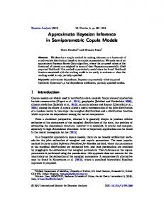
compared to the two-component case, even in terms of the exact KL distance. Note, however, that when we compare optimized trial functions with more than two components, we can of course no longer decide which one provides the best approximation in the sense of minimum KL divergence. For the numerical example of Sec. 5 we therefore focus on k = 3, although mixtures with more components could have been studied as well. Mixtures with k > 2 contain twocomponent distributions as a special case (wi = 0 for i > 2) for which W + E still provides the exact KL distance. It is therefore not unreasonable to assume that the solution of (9) for k > 2 can indeed improve upon the two-component case, and this has been observed in the example of Sec. 5. (iv) The locking condition on the covariance matrices is of course a severe restriction which has only been imposed to make the problem tractable. One can easily imagine situations in which mixtures constructed in this way will not enhance the approximation significantly. In other cases, however, appreciable improvements may be obtained. Nevertheless, as argued above, the additional computational burden is modest and the result will, in any case, be at least as good as a single-component approximation. We therefore expect that the suggested approach should in many cases provide a viable option to improve upon standard VB results in a simple way. It should also be noted that in actual computations for concrete models one essentially only needs the calculation of the energy term as a plugin, as the entropy part is independent of the specific problem. In this sense, there is no additional effort compared to single-component calculations. (v) We also note that mixtures allow us to estimate higher-order standardized moments, such as the skewness, which are inaccessible within a single-component approximation. Details of the numerical calculation of the pairwise negative entropy S¯2 = −S2 [w1 q1 , w2 q2 ] are given in Appendix A. There it is shown that S¯2 effectively depends only on λ, the Mahalanobis distance r2 = (µ1 − µ2 )T Σ−1 1 (µ1 − µ2 ), and (up to a scaling factor) the ratio of the weights w2 /w1 . The behavior of S¯2 is depicted in Fig. 3. The curves illustrate the repulsion effect between mixture components which is due to the overlap entropy and which was mentioned in the discussion of (4). This can be seen as follows. Suppose the one-component VB problem is solved by a normal distribtion q0 . In the absence of S¯2 , the twocomponent problem would then be solved by the “mixture” q¯ = 12 q0 + 21 q0 with λ = 1 and r = 0. However, as can be seen from Fig. 3, S¯2 is maximum for this mixture. The presence of S¯2 in the full two-component problem will thus tend to destabilize q¯ as minimum of the KL divergence and to make the mixture components different from each other (however, in some cases q¯ may still be the minimum of the full problem, depending on the shape of the KL landscape). Very importantly, Fig. 3(a) also shows that for growing k, S¯2 becomes more localized around λ = 1 (similar behavior is also found in the r dependence). This indicates that, in general, the differences between single- and multi-component VB solutions will be most pronounced (and hence our approach most useful) when the dimensionality of the problem is not too large.

Variational Bayes with Gaussian mixtures −

−

S2

S2 (a)

0.6

(b)

0.6

k=2

0.5

λ=1

0.5

λ=1.5

0.4

0.4 k=5

0.3 0.2

0.2

1

λ=2 λ= 0.5

0.1

k=20 0

λ= 0.67

0.3

k=10

0.1 0

367

2

3

4

λ

0

0

1

2

3

4

r

Fig 3. Behavior of negative pairwise entropy S¯2 = −S2 [equation (A.5)]. (a) Dependence on λ for r = 0, w1 = w2 = 0.5, and various k. Dashed line shows S¯2 for w1 = 0.15, w2 = 0.85. (b) Dependence on r for w1 = w2 = 0.5, k = 10, and various λ. Curve for λ = 1 is valid for all k.

3.2. Example: Multivariate generalized normal distribution To give a first illustration of the use of mixtures in VB, we now discuss a simple model problem. More elaborate and realistic applications will be studied in Secs. 5 and 6. In the present example, we consider the isotropic d-dimensional target density βΓ(d/2) p(x) = (12) exp −|x|β , d/2 2π Γ(d/β) i.e., a multivariate generalized normal distribution with shape parameter (exponent) β. The exact expression for the variance of p is given by Γ d+2 β 2 σex = . dΓ(d/β)

Due to the rotational symmetry of the target, it is a natural choice to use isotropic normal distributions N (0, σi2 I) with variances σi2 , 1 ≤ i ≤ k, in our k-component mixtures. In this way, the locking condition on the covariance matrices is fulfilled automatically. As an additional advantage, for any k we can compute the entropy of the mixture exactly in terms of one-dimensional quadratures. One can therefore easily study the effect of the approximation (9) to the original VB problem (1). For the target (12), Fig. 4 shows the results of VB calculations with single normal distributions (black curves), two-component mixtures (red), and threecomponent mixtures with the entropy treated exactly (green) and approximately (blue). We focus on the VB variances (i.e., the variances of the solutions to the VB optimization problems) which might be considered the most interesting quantities in this context from the point of view of Bayesian inference. Figure 4

368

O. Zobay

1 0.8

1 Var(VB) Var(ex.)

0.8

0.6

0.6 1 0.8 0.6 0.4 0.2 0 0

0.4 0.2 0 0

0.2

0.4 0.2 1

0.4

2

3

0.6

4

5

0.8

4 3.5

(c)

KL divergence (a)

6

7

β

1

0 0

0.2

0.4

0.8

0.6

β

1

1 (b)

Var(k comp.) Var(1 comp.)

Var(VB) Var(ex.)

0.8

(d)

d=20

3 0.6 2.5 0.4 2 0.2

1.5 1 0

0.2

0.4

0.6

0.8

. β

1

0 0

0.2

0.4

0.6

0.8

β

1

Fig 4. Variational approximation of isotropic generalized normal density (12). (a) Ratio of variationally approximated variances to exact variance as a function of exponent β for d = 5−dimensional distribution. VB approximations use k-component normal mixtures with k = 1 (black curve), k = 2 (red), k = 3 (green), k = 3 and approximation (9) (blue). Inset shows results for a larger range of β. (b) Ratio of VB variances for two- and three-component mixtures to VB variance with single Gaussian. (c) Kullback-Leibler divergences. (d) Ratio of VB variances to exact variance for d = 20-dimensional distribution. Color coding of curves in (b)-(d) corresponds to (a).

illustrates their dependence on the shape parameter β and the dimension d of the target. In addition, the KL distance is shown which can be computed exactly as the normalization constant of p is known explicitly. For the single Gaussian, the VB problem can be solved analytically, yielding the variance 2/β  dΓ(d/2)  . (13) σ12 =  β 2β/2 Γ d+β 2

In the other cases, the optimization has to be performed numerically. The overall behavior of the VB approximation is illustrated in the inset of Fig. 4(a) which


369

2 shows the ratio σ12 /σex as a function of β for a d = 5-dimensional target. For β = 2 (Gaussian target), VB is exact, but becomes less accurate the more β deviates from this value. For β > 2, i.e., for a target with light tails, it turns out that the VB approximations with two- and three-component mixtures coincide with the result from the single Gaussian. However, for β < 2, i.e., heavy-tailed targets, a very different behavior is observed. Figures 4(a) and (b), respectively, show the ratio of the various VB vari2 ances to the true value σex , and the ratio of the variances for the two- and threecomponent mixtures to σ12 . We see that the use of mixture trial functions can significantly improve the variance estimates. This enhancement is particularly pronounced for smaller values of β, where the single-Gaussian approximation becomes less and less accurate (of course, for β close to 2, single Gaussian VB becomes better so that there is less scope for improvements by using mixtures). The KL divergences shown in Fig. 4(c) behave as expected from Fig. 4(a),(b) [blue curve shows W + E of (9)]. The different types of behavior for β < 2 and β > 2, respectively, will be discussed further in Sec. 4 to exemplify the general stability criteria for single-component approximations derived there. Figure 4(d) illustrates some effects of dimensionality. One sees that for increasing d, the single-Gaussian approximation to the variance is improving. This is because for larger d the probability mass of the target tends to be localized in a shell further away from the origin, as can be seen from the behavior of the radial probability density pr (r) ∼ rd−1 p(r) with r = |x|. The distribution can therefore more easily be approximated by a Gaussian. The two- and threecomponent mixtures still provide clear improvements to the single Gaussian. However, the effect is somewhat reduced in the sense that for a given value 2 of σ12 /σex , the additional improvement from the mixtures becomes smaller for growing d. We might perhaps attribute this effect to the increasing localization of the pairwise entropies S¯2 discussed in connection with Fig. 3. It is also instructive to compare the three-component solutions for the original and the approximated VB problems (1) and (9). First of all, Fig. 4(c) shows that the approximate KL divergence W + E (blue curve) is always less than the two-component KL distance (red). As discussed above, we can therefore be sure that the approximate three-component solution improves upon the twocomponent result in the KL sense. Furthermore, we also find the KL distance for the exact three-component calculation to be less than the approximate one, as it should. Nevertheless, all four diagrams show that the differences between the exact and approximate results are very small. The neglect of the higherorder overlap contribution to the entropy is thus well justified for this example. This result is remarkable because all mixture components are centered at 0, i.e., in the present case any effects of higher-order overlap contributions should be particularly pronounced. Judging from the mixture compositions, it is also not obvious that such contributions should be negligible. To give an example, at β = 0.5, the component have variance ratios σ12 : σ22 : σ32 = 0.2 : 1 : 4 (0.46 : 1 : 2.1 for d = 20) and weights 0.24 : 0.53 : 0.23 (0.23 : 0.54 : 0.23). Based these considerations and the numerical results, we can expect that (9) will also be a useful approximation in other cases.

370

O. Zobay

4. Sufficient conditions for improvement of VB approximations by mixtures In this section, we present two simple criteria that allow us to check whether a mixture VB approximation will be guaranteed to provide an improvement compared to the single-component case. These criteria are derived from the stability analysis of the single-component minima in the KL distance with respect to mixture trial functions. We assume that the single-component minimizer of the KL divergence is given by the trial function q(θ0 ) with parameter vector θ0 . There are two ways q(θ0 ) can be “perturbed” by extending the space of trial functions to include mixture distributions: (a) by the addition of an arbitrary second component q(θ1 ) with small weight, and (b) by slightly modifying the component parameters θi around θ0 in a mixture with arbitrary weights. The first possibility corresponds to a stability analysis with trial functions (1 − δw)q(θ0 ) + δwq(θ P 1 ) and δw ≪ 1, whereas for the second option trial functions of the form i wi q(θ0 + δθi ) with small δθi are considered. We will discuss both situations in turn and derive corresponding criteria for the instability of the single-component solution. In order to examine the first case, we consider the mixture (1 − w)q(θ0 ) + wq(θ1 ). Its KL divergence is given by KL(w; θ0 , θ1 |p) =

Z

[(1 − w)q(θ0 ) + wq(θ1 )] log [(1 − w)q(θ0 ) + wq(θ1 )] Z − [(1 − w)q(θ0 ) + wq(θ1 )] log p

with p the target distribution. Assuming exchangeability of integration and differentiation, the first two derivatives of the KL divergence with respect to w read Z ∂w KL = [−q(θ0 ) + q(θ1 )] log [(1 − w)q(θ0 ) + wq(θ1 )] (14) Z − [−q(θ0 ) + q(θ1 )] log p, (15) ∂ww KL

=

Z

2

[−q(θ0 ) + q(θ1 )] . (1 − w)q(θ0 ) + wq(θ1 )

(16)

Taking the limit w ↓ 0, the (one-sided) derivative of the KL divergence at w = 0 is found as ∂w KL |w=0 = KL(θ1 |p) − [KL(θ1 |θ0 ) + KL(θ0 |p)] .

(17)

The instability of the single-component minimum of the KL divergence with respect to the admixture of component q(θ1 ) is therefore guaranteed if expression (17) is negative. This condition can be checked very easily in practical calcula-


371

tions4 and thus be used in the search for good starting values for the iterative optimization of the mixture approximation. Note that if the KL divergence were to fulfill a triangle inequality, (17) would always be non-positive. However, as this is not the case, (17) can be both negative and positive. It should also be noted that the second derivative (15) is non-negative for all values of w. This implies that that for KL(θ0 |p) < KL(θ1 |p) and positive first derivative (17) at w = 0, all mixtures (1 − w)q(θ0 ) + wq(θ1 ) have larger KL divergence than q(θ0 ). This holds independent of whether q(θ0 ) is the actual single-component minimizer. For the example of Sec. 3.2 involving an isotropic generalized normal target distribution approximated by isotropic Gaussians, criterion (17) can be evaluated analytically. Choosing q(θ0 ) as the single-component minimizer determined by (13), it is found that for β < 2 and any d, (17) is negative for any q(θ1 ), i.e., q(θ0 ) is always unstable against admixture of a second component. For β > 2, however, (17) is always positive. In particular, this implies that any mixture (1 − w)q(θ0 ) + wq(θ1 ) has a larger KL divergence than q(θ0 ). Nevertheless, this argument does not rule out that mixture distributions not involving q(θ0 ) may have a lower KL divergence. This can only be checked numerically. We now turn to the second way of perturbing the single-component solution which involves modification of the component parameters. Let Q(1) be a family of trial functions q(θ) which smoothly depend on the p-dimensional parameter vector θ. The KL distance KL(1) (θ) to the target function p and the first two derivatives of KL(1) with respect to θ are given by Z Z KL(1) (θ) = q(θ) log q(θ) − q(θ) log p, (18) Z Z ∂θ KL(1) (θ) = ∂θ q(θ) log q(θ) − ∂θ q(θ) log p, (19) ∂θθ KL(1) (θ)

=

A(θ) + B(θ)

with the matrices A(θ) and B(θ) defined by Z Z A(θ) = ∂θθ q(θ) log q(θ) − ∂θθ q(θ) log p, Z 1 ∂θ q(θ)[∂θ q(θ)]T . B(θ) = q(θ)

(20)

(21) (22)

Let θ0 be the global minimizer of KL(1) (θ), assumed to lie within the interior of the parameter space. This implies that ∂θ KL(1) (θ0 ) = 0. We assume that the matrix of second derivatives ∂θθ KL(1) (θ0 ) is positive definite, thus excluding some exceptional cases. 4 The difference KL(θ |p) − KL(θ |p) is available from the single-component computations. 1 0 In case p is of the form p(x|y) = p(x, y)p(y), the potentially problematic evidence terms − log p(y) in the KL divergence cancel. The KL divergence KL(θ1 |θ0 ) can be derived analytically for Gaussian trial functions.

372

O. Zobay

We now consider the family Q(k) of k-component mixture distributions derived from Q(1) and characterized by parameters (θ(1) , . . . , θ(k) ) and weights (k) w1 , . . . , wk . The set Q0 of functions within Q(k) that are equivalent to the (1) single-component minimizer q(θ0 ) have P constrained parameters (θ = θ0 , . . . , (k) θ = θ0 ) but unrestricted weights i wi = 1. (k) In the following, we first show that the functions in Q0 are stationary points of the k-component KL distance KL(k) . We then investigate the stability of these stationary points with respect to variations of the θ(i) . It turns out that the stability depends on the eigenvalues of the matrix A(θ). If A has negative eigenvalues, the stationary points will be unstable. This means that the global minimum of KL(k) is less than KL(1) (θ0 ), i.e., the mixture distributions are guaranteed to lead to an improved approximation compared to the single-component case. If all eigenvalues are strictly positive, the k-component stationary points will be stable, i.e., they form a local minimum. In this case, the local stability analysis cannot predict anything about the possible improvements by mixtures, as we cannot decide whether these local minima are also global. In the marginal case of A having positive and zero eigenvalues, we also cannot draw any conclusions. Note that this discussion is independent of the number of mixture components. More formally, these results are summarized as follows (proofs are provided in Appendix B). (k)

Theorem 1. The functions in Q0 KL(k) .

are stationary points of of the KL distance

The independence of KL(k) on the wi ’s also directly implies that ∂wj wl KL(k) = 0 and ∂θ(j) ,wl KL(k) = 0. The stability of the stationary points is therefore determined by the matrix ∂θ(j) ,θ(l) KL(k) . (k)

Theorem 2. For the functions in Q0 , k i h Y (k) k−1 wi = (det A) det(A + B) det ∂θ(j) ,θ(l) KL

(23)

i=1

with A and B defined in (21) and (22) with θ = θ0 . At w1 = · · · = wk = 1/k, the eigenvalues λ of ∂θ(j) ,θ(l) KL(k) are the roots of the characteristic equation [det(A − kλ1p )]k−1 det(A + B − kλ1p ) = 0

(24)

with 1p the p-dimensional identity matrix. Corollary 1. If A has negative eigenvalues, the global VB optimizer in the class Q(k) of k-component mixture distributions is guaranteed to improve upon the best single-component approximation q(θ0 ). Corollary 2. If all eigenvalues of A are positive, the KL divergence KL(k) has a local minimum at the k-component mixture distributions corresponding to the best single-component solution q(θ0 ).


373

To illustrate these results, we again apply them to the example discussed in Sec. 3.2. In this case, the parameter vector θ is one-dimensional and only contains the variance σ 2 of the isotropic Gaussian trial function. The determinant det(A(θ0 )) at the minimizer θ0 of the single-component problem be calculated analytically. It is found to be proportional to 2 − β, with β the shape parameter of the target. Corollaries 1 and 2 thus imply that for β < 2, mixture trial functions are guaranteed to provide an improvement, whereas for β > 2 the single-component solution remains a local minimum. These conclusions are in agreement with the results obtained from criterion (17) and are confirmed by the numerical calculations described in Sec. 3.2. In particular, for β > 2 the results suggest that the single-component solution is in fact the global minimum, as no better approximation could be found. We conclude this section with a brief comment on the application of the criteria to the shape- and orientation-locked Gaussian mixture trial functions described in Sec. 3.1. Here one should keep in mind that the parameter vector θ cannot contain the unconstrained covariance matrix due to the locking condition. To simplify the practical use of the criteria, one could therefore consider mixture components N (µ, βΣ0 ) where only µ and the scalar β are variable parameters. The covariance matrix Σ0 would be kept fixed, e.g., at the result for the single-component minimizer. 5. A non-Gaussian state-space model Following the study of an illustrative example with an isotropic target density in Sec. 3, we now investigate a non-Gaussian linear state-space model as a more realistic application of the mixture method. The choice of this model is partly motivated by the results of Sec. 3.2, where we found that the use of mixtures can provide appreciable improvements for heavy-tailed target distributions. However, it should be emphasized that the approach can be applied to any model that is amenable to VB treatment with a single Gaussian. As is common with variational calculations, the potential benefits are very difficult to gauge a priori, and empirical studies are needed, in general. Our non-Gaussian state-space model for the random variables X1:n and Y1:n is defined by Xi+1 = φXi + ηi , Yi = Xi + ξi ,

ηi ∼ GN (0, β, κ),

ξi ∼ GN (0, α, ρ),

(25) (26)

where we have set X0 ≡ 0. Here, GN (β, µ, κ) denotes the (univariate) generalized normal distribution with mean µ, shape and scale parameters β and κ, respectively, and density " β # |x − µ| β . exp − pgn (x; µ, β, κ) = 2κΓ(1/β) κ

(27)

374

O. Zobay

The complete probability distribution for the model is thus given by p(x1:n , y1:n ) =

n Y

pgn (xi ; φxi−1 , β, κ)pgn (yi ; xi , α, ρ).

(28)

i=1

In the following, we will assume that the model parameters (α, β, κ, ρ, φ) are known, and that data y1:n have been observed. The objective is then to study the posterior distribution p(x1:n |y1:n ). In the VB treatment of this model, we will compare the approximation using a single Gaussian to two- and threecomponent mixtures. The three-component calculation is based on the modified VB optimization problem (9). Details of the variational calculations are given in Appendix C. We note that the dimensionality of the minimization problem scales linearly with the number of observations. To assess the overall accuracy of the variational results, we have also performed MCMC calculations using a standard Gibbs sampling approach. Draws from the corresponding univariate conditional densities are obtained using adaptive rejection Metropolis sampling (Gilks, Best and Tan 1995). In the subsequent discussion, we will focus on the variational results for mean, variance, and skewness. In particular, it should be emphasized that the skewness (or any other higher-order moment) cannot be obtained from single-component VB, but becomes accessible through the mixture approach. In view of the fact that nonparametric variational calculations would be very difficult for the given model, we can thus conclude that Gaussian-mixture VB provides a genuine extension of the capabilities of variational calculations. Our numerical studies of the model (25), (26) confirm some general trends which are already observed in the simple example of Sec. 3.2. It is found that the mixture approach is most effective for heavy-tailed distributions (i.e., α and β less than 2) and moderate dimensionality (i.e., number n of observations not too large). In the subsequent numerical examples, we will therefore focus on the case of equal shape parameters α = β for which the values 1.2 and 0.35 are chosen in two sets of calculations. The other model parameters are kept fixed at κ = 1, ρ = 0.2, and φ = 0.5. The observations y1:n are generated from the model (25), (26) with the given parameters and n set to 5 or 15. For each parameter setting, 200 random samples are investigated in order to get an overview of the performance of the approach. The main findings can be summarized as follows. In all cases, mixture VB reduces the KL divergence, i.e., it improves the approximation of the posterior. MCMC means are reproduced quite accurately already with a single Gaussian. VB tends to underestimate variances, but the mixture approach increases single-component results by up to 30% on average depending on parameters, with larger increases for smaller samples and growing non-Gaussianity. The variational skewness estimates usually reproduce the sign of the MCMC results although they tend to underestimate the actual value. For a more detailed discussion, we first turn to the case α = β = 1.2 for which VB calculations of posterior variance and skewness are shown in Fig. 5


375

Fig 5. Variational study of non-Gaussian state space model (25), (26) for parameters α = β = 1.2, κ = 1, ρ = 0.2, φ = 0.5 and number of observations n = 5 (a,b) and n = 15 (c,d). For both parameter settings, 200 random samples generated from the model were investigated. Figures (a) and (c) show the ratio V3 /VM C of marginal variances calculated from three-component VB and MCMC as a function of V1 /VM C with V1 the variance from the single-component calculation. Red lines show diagonal y = x. These diagrams illustrate the change in the estimated variance when using mixture VB. Figures (b) and (c) depict the skewness ratio γ3 /γM C as a function of the standardized third moment τM C as obtained from MCMC.

(means will be briefly mentioned in the discussion of Fig. 7 which refers to α = β = 0.35). Results for the variance are shown in Figs. 5(a) (n = 5) and 5(c) (n = 15). The diagrams depict the variance ratio V3 /VMC as a function of V1 /VMC . Here, V1 and V3 denote the variance of a specific posterior marginal p(xi ) as calculated from one- and three-component VB, whereas VMC is the corresponding MCMC result. We see that the single-component results are already quite accurate as V1 /VMC ranges from 0.85 to 0.95 (note that variances are underestimated as discussed in Sec. 2.1). All points in Figs. 5(a) and (c) lie between the diagonal y = x (red line) and the horizontal y = 1. This means that in all cases V1 < V3 < VMC , i.e., the three-component calculation always provides an improved estimate of the variance. As V1 already yields a very good approximation, the improvement is not large, but nevertheless clearly obvious and significant. We also see that for growing n the average improvement is re-

376

O. Zobay

duced, e.g., for V1 /VMC ≈ 0.90 we find V3 /VMC to approximately range within 0.934 ± 0.005 for n = 5 and 0.912 ± 0.002 for n = 15. The benefits of the mixture calculation become even more obvious when studying the results for the skewness as this quantity cannot be obtained from single-Gaussian VB. Skewness is defined as γ=

τ V 3/2

(29)

with V the variance and τ = E[(X − E(X))3 ] = E(X 3 ) − 3E(X 2 )E(X) + 2E(X)3 the third moment about the mean. In Figs. 5(b),(d) (for sample sizes n = 5 and n = 15, respectively), the VB-to-MCMC skewness ratio γ3 /γMC is shown as a function of the third moment τMC obtained from MCMC. We first of all find that the VB calculation provides a reliable estimate of the overall skew of the posterior (i.e., the sign of γ). In both calculations, one finds that in only about 5% of all cases the ratio γ3 /γMC is negative, i.e., γ3 and γMC have opposing signs. As can be seen from the diagrams, these discrepancies predominantly occur when |τMC | is small. This behavior can be explained by the fact that for small |τ |, the estimate of τ will be very sensitive to any errors in the (MCMC or variational) calculations of the moments E(X j ). For larger |τMC |, most VB results appear to underestimate γMC by an almost constant factor (about 0.3 in (b) and 0.1 in (d)). However, there is also a distinct group of cases for which the ratio γ3 /γMC becomes close to one. Altogether, we thus find that mixture VB provides a useful first approximation of posterior skewness. Results for the case of α = β = 0.35 are displayed in Figs. 6 and 7. Figures 6(a),(b),(d),(e) show variance ratios for n = 5 and n = 15, with (b) and (e) providing enlargements of (a) and (d), respectively, for small V1 /VMC . For α = β = 0.35, the model exhibits much stronger non-Gaussianity than in the previous case and consequently the VB approximation becomes less accurate. As can be seen from Figs. 6(a) and (d), the variance ratio V1 /VMC extends over a much larger range extending from 0 to 1 with most values, however, in the region of small V1 /VMC . For small ratios V1 /VMC , Figs. 6(b) and (e) indicate that mixture VB brings about a marked improvement in the estimation of the variances. We also see that for small V1 /VMC , we have only a few cases with V3 < V1 . However, this behavior changes as V1 /VMC becomes larger as estimates with V3 < V1 occur more often. More specifically, 66% of all cases for n = 5 (68% for n = 15) have V1 /VMC < 0.5. For 92% (96%) of these cases, the mixture approximation improves the variance estimates, i.e., V3 > V1 . The extent of improvement, as measured by mean of the variance ratio V3 /V1 , is 1.49 (1.13). When we consider all cases, the percentages decrease to 73% (83%) and the ratios to 1.31 (1.08). It thus appears as if the benefits of the mixture approximation are strongest where single-component VB performs badly (i.e., small V1 ), at the expense of reduced improvement where single-component VB is good already. At any rate, it should be kept in mind that for every sample the KL divergence of the mixture approximation is lower than the single-component value, i.e., the overall approximation of the posterior is improved even if some variance estimates become somewhat less accurate.


377

Fig 6. Variational study of non-Gaussian state space model (25), (26). Parameters as in Fig. 5 except for α = β = 0.35. Number of observations are n = 5 (a,b,c) and n = 15 (d,e,f ). Diagrams show variance and skewness ratios obtained for 200 random samples analogous to Fig. 5. Figures (b) and (e) depict detail of (a) and (d), respectively, for small V1 /VM C .

The overall skew is still determined correctly in about 77% of all cases (i.e., γ3 and γMC have the same sign). As can be expected, Figs. 6(c) and (f) show that the skewness ratios γ3 /γMC are lower than in the case of α = β = 1.2. Altogether, the results show that the application of mixture VB still remains useful in the study of this model.

378

O. Zobay

Fig 7. Variational calculation of marginal means. Parameters as in Fig. 6 with n = 5. (a) Marginal mean µM C calculated with MCMC as a function of the corresponding observation yi . (b) Ratio µ3 /µM C as a function of µ1 /µM C with µ1 and µ3 marginal means obtained from one- and three-component VB.

Finally, Fig. 7 displays some results on the posterior means for α = β = 0.35. In order to provide an additional perspective on the model, Fig. 7(a) shows the ratio µMC /yi of the posterior mean µMC evaluated from MCMC and the actual observation yi as a function of yi itself. As might be expected from the model structure, the posterior mean is very close to yi for large |yi |, but becomes more variable and typically smaller in modulus than yi when yi tends towards 0. The histogram shows the frequency distribution for the values of the ratio µMC /yi . Figure 7(b) indicates that the VB estimation of the posterior means is typically very accurate even in this case of strong non-Gaussianity. In almost 90% of all cases, µ1 /µMC lies between 0.8 and 1.2. Mixture VB does not provide an obvious benefit in this regard as µ1 and µ3 are mostly very close to each other. For α = β = 1.2 it is found that the spread in µ1 /µMC and µ3 /µMC is even further reduced (between 0.97 and 1.03). 6. The Bayesian lasso In sparse regression, one solves the minimization problem p n X X P (|βj |, λ) L(yi − µ − xi β) + min (µ,β )∈Rp+1 i=1 j=1

(30)

in order to obtain shrinkage estimates for the regression coefficients β. In (30), (y1 , . . . , yn )T ≡ y are observations, µ is an overall mean and xi a row of the n×p-dimensional design matrix X. The loss function to be minimized is denoted L, and P is a penalty function that shrinks the estimates towards zero. The amount of shrinkage is controlled by the penalty parameter λ. The popular lasso is obtained for quadratic loss and the penalty function P (|βj |, λ) = λ|βj | (Tibshirani 1996).


379

Recently, Bayesian versions of sparse regression have attracted considerable attention (see, e.g., Park and Casella (2008), Hans (2009; 2010)). In the Bayesian formulation, the loss function is used to construct the data likelihood while the penalty gives rise to a prior for β. For certain models, for example the Bayesian lasso, it has been possible to derive efficient MCMC samplers (Park and Casella 2008, Hans 2009). However, these samplers usually rely on sophisticated methodology, and for other models it may not be obvious how to construct suitable sampling schemes. For example, Park and Casella (2008) discuss a “Huberized” lasso for which MCMC sampling of a one-to-one Bayesian translation appears difficult. In such situations, variational Bayesian inference with Gaussian trial functions might present an interesting alternative. Consider, e.g., a Bayesian sparse regression problem with a multivariate normal data P likelihood (derived from a quadratic loss L) and a prior distribution exp[− j P (|βj |, λ)]. For Gaussian trial functions, it is straightforward to compute the contribution of the data likelihood to the energy R part of the KL divergence. The prior gives rise to one-dimensional integrals N (β; µ, σ 2 )P (|β|, λ)dβ which either may be solved analytically or can be evaluated numerically using Gauss-Hermite integrals. If such an approach turns out to be feasible, it is natural to ask what improvements in accuracy are afforded by using Gaussian mixtures as trial functions. In the following, we will discuss this question for the Bayesian lasso. This model provides a convenient example as the availability of efficient MCMC samplers makes it easy to compare the variational approximations to Monte-Carlo results. The computational gain of the variational method is not too pronounced in this case, but for other models the variational approximation should provide a clear advantage. The Bayesian lasso is defined as y|µ, β, σ 2 2

∼

βi |σ , λ ∼ µ ∼

N (µ1n + Xβ, σ 2 In ), √ Laplace(0, σ 2 /λ), 1.

(31) (32) (33)

√ 2 Laplace(0, √ 0 and scale pa√ σ /λ) denotes the√Laplace distribution with mean 2 rameter σ /λ, i.e., pL (x; 0, σ 2 /λ) = λ/(2σ 2 ) exp(−λ|x|/ σ 2 ). In order to compute inferences for β, it is convenient to center y and standardize X. With a flat prior, the parameter µ can then be marginalized out (Park and Casella 2008) and is ignored in the following. It is straightforward to impose priors on λ and σ 2 , but in order to work out the effects of the mixture trial functions as clearly as possible, these parameters will be assumed known. Specifically, σ 2 is set equal to its estimate from standard linear regression whereas λ is treated as a variable external parameter. Details of the variational calculations are given in Appendix D. Data from a diabetes study (n = 442, p = 10) have been used in numerical examples in a number of papers on the lasso and its Bayesian version (e.g., Efron, Hastie, Johnstone and Tibshirani (2004), Park and Casella (2008), Hans (2009)) and will also be considered in the following. More specifically, we study the behavior of the variational approximations as the penalty parameter λ is

380

O. Zobay

0.6

(a)

Scaled Mean(β4)

Change in KL

0 −0.05 −0.1 −0.15 −0.2 50

100

λ

0.6 0.4 0.2 100

λ

100

λ

1

0.5

200

(d)

0.06 0.04 0.02 100

λ

0

(e)

150

0.08

0 50

200

Skew( β7)

Skew( β4)

1.5

150

0.2

0.1

(c)

0.8

0 50

0.4

0 50

200

Scaled Var( β7)

Scaled Var( β4)

1

150

(b)

150

200

(f)

−0.5 −1 −1.5

0 50

100

λ

150

200

50

100

λ

150

200

Fig 8. Variational inference for the Bayesian lasso with diabetes data. Black, red and blue curves pertain to variational approximations with one, two, and three Gaussians, respectively, green curves are MCMC results. (a) Decrease in KL divergence. (b)-(f ) Means, variances and skew for posteriors of parameters β4 and β7 . Means and variances are scaled to values from ordinary linear regression.

varied. Figure 8 summarizes the calculations. Variational results for a single Gaussian and two- and three-component mixtures are shown in black, red and blue, respectively, while green curves pertain to MCMC. Figure 8(a) displays the decrease in KL divergence compared to the single-Gaussian solution. Given that the maximum possible gain in KL from a two-component mixture equals log 2 ≈ 0.69 (Jaakkola and Jordan 1998), Fig. 8(a) indicates that even with the locking constraint two-component VB provides an appreciable and consistent improvement over the single-component approximation. The gain increases with growing λ up to values around 0.13 for λ ≈ 200. The three-component solution provides further improvement mainly for larger values of λ.


381

Figure 8(b) shows a representative result for the mean value of the β posteriors, here for the example of parameter β4 (blood pressure) normalized to its value at λ = 0. Typically, the one-component mean already provides a very good approximation to the MCMC result so that the further improvements by the mixture solutions are small. For the variance, the difference between variational and MCMC calculations becomes larger. For some regression parameters, the mixture results show noticeable improvements, for example for the parameters β4 and β7 (Figs. 8(c,d)). Compared to the single-component solution, the relative increases in variance are between 10 and 50% at larger λ’s. Note, in paticular, the additional improvement for the three-component solution in 8(d). For most of the other parameters, the relative increase in variance is smaller and of the order of a few percent. For most parameters, the variational approximation of the skew correctly predicts the sign but underestimates the actual value, similar to what was found in Sec. 5. Results for β4 and β7 are shown in Figs. 8(e) and (f). The relatively close agreement of the three-component solution with MCMC in Fig. 8(f) is unusual. Parameters β3 and β9 show somewhat different behavior, there the MCMC skew stays close to 0 whereas VB predicts values around −0.1. The KL distance for the mixture trial functions typically has more than one local minimum. In the two-component case, another solution was found5 which has a smaller KL divergence at smaller λ, i.e., at these values it provides a better overall approximation. Compared to the single-component result, it improves the moments of the posterior marginals mainly for β8 with the other parameters remaining almost unchanged. As the solutions of Fig. 8 mainly enhance β4 and β7 , these observations suggest that the mixture approximations tend to focus their impact on a subset of parameters. This impression was confirmed in calculations with other data sets where mixtures typically increased variance estimates by up to 10% for most parameters, but significantly larger increases were observed for some parameters. For the calculations of Fig. 8, the computation time for two- and threecomponent optimizations was increased by factors of about 3.3 and 10.4 on average compared to one-component runs (which took about 1.2 seconds on average). However, since the most time-consuming contribution comes from calculating the KL distance these factors can be expected to vary from problem to problem. For the lasso, the energy computations were almost instantaneous compared to the mixture entropy (the hypergeometric function was linearly interpolated from a dense precomputed grid). In other cases, the energy computations may be much more time-consuming thus modifying the time ratios. Another aspect that might warrant further exploration are the convergence criteria of the VB optimization routine. In particular for mixtures, it often appeared that before stopping many iterations were performed with very little change in the KL divergence. Computing 100,000 iterations of the MCMC sampler of Park and Casella (2008) in the same computational environment took about 12 seconds. 5 The discontinuity in the three-component results in Fig.8 (blue curves) around λ = 70 is also due to a switch between different families of solutions.

382

O. Zobay

7. Summary and conclusions An important objective of current research on Variational Bayesian methods is to develop and investigate improved approximation schemes. In this context, the purpose of the present paper is to study the use of Gaussian mixture distributions as trial functions. The main results can be summarized as follows. (i) The key problem regarding the use of mixtures as trial functions is the calculation of the entropy which becomes analytically intractable. In the present work, this obstacle was overcome with the help of a lower-bound approximation to the entropy in terms of all contributions from individual components and their pairwise combinations. (ii) Even for Gaussian mixtures, the pairwise combinations still cannot be calculated analytically. In order to make practical calculations feasible, “shape- and orientation-locking” constraints were imposed on the Gaussian covariance matrices so that the entropy approximation could be computed by standard two-dimensional numerical integration. (iii) Two simple sufficient criteria were derived that permit to check if a mixture approximation is guaranteed to provide an improvement to single-component VB. (iv) To illustrate the method, three examples were discussed in detail with target distributions chosen as isotropic generalized normal distributions, a non-Gaussian state space model and the Bayesian lasso, respectively. These examples suggest that for heavy-tailed distributions, Gaussian-mixture VB can be expected to indeed lead to an improved approximation of the target distribution in the sense of a reduced KL divergence. Appreciable improvements for posterior variance estimates could be obtained already with two- and three-component mixtures. In addition, it was shown that mixture VB provides an estimate of skewness, which is impossible for single-component Gaussian VB. A major objective for further methodological work on the mixture approach is the development of more flexible ways to calculate the mixture entropy that allow us to overcome the current restriction to “shape- and orientation-locked” Gaussians. The calculation of Gaussian mixture entropies is a topic of ongoing research to which no final solutions have been found yet. However, in the present context the problem is alleviated to some degree by the fact that only the entropy of two-component mixtures is required, in contrast to the general k-component problem. This should make it easier to find more general numerical or even analytical approximations. The numerical examples suggest a potential limitation of the approach in the form of a reduced effectiveness for higher-dimensional target distirbutions. This behavior might at least in part be due to the restrictions on the Gaussian covariances imposed by the locking condition; however, it is also found for the isotropic target of Sec. 3.2 where these restrictions should be less of an issue. A possible qualitative explanation might be given by the reduction in the “entropic repulsion” discussed in Sec. 3.1. Further work and investigation of additional examples is necessary to clarify this issue. However, it should be kept in mind that VB can be of significant practical value even in lower-dimensional problems. Due to the relative speed advantage compared to MCMC, considerable gains in absolute computation time can be obtained if a larger number of inference prob-


383

lems has to be solved. An example for such a situation is given by the inferences for multipe values of the penalty parameter in sparse regression, see Sec. 6. Another interesting lower-dimensional application of the present approach might be found in semiparametric VB approximations when the Gaussian factor remains of lower dimension. Regarding the practical aspects of mixture VB calculations, it should be emphasized that the mixture entropy calculations need to be coded only once in a problem-independent way, and the method then requires no further essential adaptations to specific targets, except for what is already needed for the singlecomponent calculations. It is hoped that the modest implementation effort and the potential gain in accuracy outweigh the increase in computation time and make the method an interesting, practically viable option for improving VB calculations. Acknowledgements Valuable comments and suggestions by two anonymous referees and the Associate Editor are gratefully acknowledged. This work was supported by an EPSRC Statistics Mobility fellowship.

Appendix A: Numerical calculation of pairwise entropy In the following, we outline the numerical calculation of the pairwise entropy contribution S2 defined in (4) for multivariate normal distributions under the locking condition. Essentially, one needs the integral w2 N (x; µ2 , Σ2 ) . dx1:k N (x; µ1 , Σ1 ) ln 1 + w1 N (x; µ1 , Σ1 ) (A.1) −1 T T We now define the matrix U as square root of Σ−1 1 , i.e., Σ1 = U U with U the transpose of U , and set µ := µ1 − µ2 . Using these definitions, the above integral can be transformed to the “normal form” Z

I(µ1 , µ2 , Σ1 , Σ2 , w1 , w2 ) =

w2 N (x; U µ, U Σ2 U T ) dx1:k N (x; 0, I) ln 1 + w1 N (x; 0, I) (A.2) with I the identity matrix. We now invoke the locking condition Σ2 = λ2 Σ1 which simplifies the above expression to I(µ1 , µ2 , Σ1 , Σ2 , w1 , w2 ) =

I(µ1 , µ2 , Σ1 , Σ2 , w1 , w2 ) =

Z

Z

w2 N (x; U µ, λ2 I) . (A.3) dx1:k N (x; 0, I) ln 1 + w1 N (x; 0, I)

The integral can now be evaluated in cylindrical coordinates (ρ, z) with the cylinder axis directed along U µ. This yields

384

I

O. Zobay ∞

∞

1 2 2 p dz dρ Ωk−1 ρ exp − (z + ρ ) 2 (2π)k −∞ 0 1 1 2 1 −2 w2 2 2 (A.4) exp − 2 (z − r) + z − (λ − 1)ρ × ln 1 + w1 λk 2λ 2 2

Z

=

Z

1

k−2

with Ωk−1 = 2π (k−1)/2 /Γ((k−1)/2) the surface area of a (k−1)-dimensional unit sphere. Furthermore, r = |U µ| which is readily evaluated from r2 = µT Σ−1 1 µ. Due to the presence of the Gaussian weight function, the integral (A.4) can very efficiently be computed using generalized Gauss-Hermite quadrature. In typical calculations, we use 20 grid points for z and 10 points for (positive) ρ. To save computation time, only (z, ρ) grid points are considered for which the product of the quadrature weights is larger than a cutoff of 10−8 . One might also consider schemes with variable accuracy which is increased once the calculation approaches convergence. For conjugate gradient minimization, one also requires the partial derivatives of I with respect to λ, wi , and r. These are readily obtained by differentiating the integrand in (A.4). Equation (A.4) shows that the integral I depends only on the parameters r, λ and the ratio ω = w2 /w1 , i.e., I = I(λ, ω, r). The total negative pairwise entropy S¯2 = −S2 [w1 q1 , w2 q2 ] is then given by S¯2 [w1 q1 , w2 q2 ] = w1 I(λ, ω, r) + w2 I(λ−1 , ω −1 , r/λ).

(A.5)

Appendix B: Proofs of Theorems and Corollaries in Section 4 (k)

Proof of Theorem 1. The functions in Q0 P w i i = 1, wi ≥ 0. For these functions (k)

∂θ(j) KL

=

Z

wj ∂θ q(θ0 ) log

" X i

are given by

P

i

wi q(θ(i) = θ0 ) with

#

wi q(θ0 )

Z 1 wj ∂θ q(θ0 ) − wj ∂θ q(θ0 ) log p i wi q(θ0 ) i Z Z = wj ∂θ q(θ0 ) log q(θ0 ) − ∂θ q(θ0 ) log p = 0, +

Z X

wi q(θ0 ) P

the bracket in the last line vanishing because θ0 is a stationary point of the singlecomponent KL distance. As KL(k) does not depend on wi for the functions in (k) Q0 , we can immediately conclude that ∂wj KL(k) = 0. Proof of Theorem 2. Straightforward calculation shows that ∂θ(j) ,θ(l) KL(k) = diag(w1 , . . . , wk ) ⊗ A + wwT ⊗ B

= diag(w1 , . . . , wk ) ⊗ A T w1 B 1/2 , . . . , wk B 1/2 , (B.1) + w1 B 1/2 , . . . , wk B 1/2


385

with w a column vector containing the weights wi , B = B 1/2 B 1/2 and ⊗ the Kronecker matrix product. We can now make use of the general matrix identity det(M + QT Q) = det 1s + QM −1 QT det M for r × r-dimensional, invertible M and s × r-dimensional Q with arbitrary r and s. Assuming for now that A and B are invertible, we can apply this identity to (B.1) to obtain det ∂θ(j) ,θ(l) KL(k)

=

det 1p + B

1/2

−1

A

B

1/2

k X

wi

i=1

=

!

(det A)k

k Y

wi

i=1

k i h Y wi det B 1/2 B −1 + A−1 B 1/2 (det A)k i=1

=

k Y wi det B B −1 + A−1 A (det A)k−1 i=1

=

(det A)k−1 det(A + B)

k Y

wi

(B.2)

i=1

which proves (23) for invertible A and B. However, due to continuity (23) also holds in case A or B are not invertible. To show (24), we need to study the characteristic polynomial det(∂θ(j) ,θ(l) KL(k) − λ1kp ) at wi = 1/k. However, brief inspection of (B.1) reveals that we can evaluate this determinant in the same way as above if we replace A by A − k1p in (B.1). This immediately yields (24). Proof of Corollary 1. The k-component mixture with (θ(1) = θ0 , . . . , θ(k) = θ0 ) and w1 = · · · = wk = 1/k describes the same distribution as q(θ0 ), its KL divergence equalling KL(1) (θ0 ). However, from (24) and the assumption on A it follows that its stability matrix has negative eigenvalues, i.e., the KL divergence KL(k) has a saddle point at this distribution. Hence, the global minimum of KL(k) must lie below the minimum of KL(1) (θ0 ). Proof of Corollary 2. Consider first the case k = 2. From (24) follows that the stability matrix for the mixture distribution with (θ(1) = θ0 , . . . , θ(k) = θ0 ) and w1 = · · · = wk = 1/k has only positive eigenvalues. By the implicit function theorem, the eigenvalues of the stability matrix are continuous functions of the weights w1 and w2 . As long as w1 and w2 are both different from zero, (23) thus guarantees that the eigenvalues will remain positive, as the determinant cannot become zero. If w1 = 0 or w2 = 0, we have a one-component distribution which is already known to minimize the KL distance under variation of θ. For k > 2, we can prove the corollary inductively. As long as all mixture weights are different from zero, the positivity of the eigenvalues of the stability matrix follows in the same way as in the case of k = 2. If one or more weights are zero, the distribution corresponds to a mixture with a number of components less than k, and the positivity of the eigenvalues follows from the induction hypothesis.

386

O. Zobay

Appendix C: Variational calculations for non-Gaussian state-space model To compute the energy term of the KL divergence we need the integral Z N (x1:n ; µ, Σ) ln p(x1:n |y1:n )dx1:n Z = N (x1:n ; µ, Σ) ln p(x1:n , y1:n )dx1:n − ln p(y1:n )

(C.1)

with N (x1:n ; µ, Σ) the n-dimensional normal distribution with mean µ and covariance matrix Σ. As the evidence p(y1:n ) is not known analytically, we can only compute the first term on the right-hand side of (C.1). Therefore, we cannot evaluate the actual KL divergence; rather, the optimization problem will eventually provide a lower bound on the evidence. Using (28), we obtain from (C.1) Z N (x1:n ; µ, Σ) ln p(x1:n , y1:n )dx1:n =

Z

N (x1:n ; µ, Σ)

n X

[ln pgn (xi ; φxi−1 , β, κ) + ln pgn (yi ; xi , α, ρ)] dx1:n

i=1

α β = n ln 2κΓ(1/β) 2ρΓ(1/α) Z n Z X − κ−β N (x1 ; µ1 , Σ11 )|x1 |β dx1 − ρ−α N (xi ; µi , Σii )|yi − xi |α dxi

i=1

− κ−β

n Z X i=2

N (xi−1:i ; µi−1:i , Σi−1:i )|xi − φ xi−1 |β dxi−1:i

(C.2)

where the normal distributions for xi and xi−1:i in the last two lines refer to the corresponding marginals of N (x1:n , µ, Σ). The two one-dimensional integrals in the second-to-last line of (C.2) can be solved analytically in terms of confluent hypergeometric functions using the relation r Z γ 1 µ2i 1+γ (2σ 2 )γ 2 γ (C.3) Γ N (x, µ, σ )|x| dx = 1 F1 − , , − π 2 2 2 2σ 2 (obviously, as a function of µ the right-hand side simply provides a smoothed version of |µ|γ ). For the computation of the confluent hypergeometric function 1 F1 , efficient numerical routines are available (Zhang and Jin 1996). To evaluate the double integral of (C.2) involving xi−1 and xi , we first integrate out one variable analytically using (C.3) and then perform the second integration using Gauss-Hermite quadrature. Equation (C.2) shows that the energy only depends on the elements Σi,i and Σi±1,i of the covariance matrix Σ. For VB with a single Gaussian, (11)


387

thus implies that the inverse of the optimized covariance matrix will be tridiagonal. The single-Gaussian VB problem therefore involves the optimization of an n-component mean vector µ and a covariance matrix Σ depending on 2n − 1 parameters. For VB with mixtures, there is no equivalent to relation (11) that would impose a restriction on the form of the optimized covariance matrix. However, the numerical calculations show that, at least under the locking condition, the optimized inverse covariance matrices retain the band structure form to a very good degree of approximation. It is therefore reasonable to impose this constraint from the outset to simplify calculations. In this way, VB with two components results in a 4n + 1-dimensional optimization problem (2n parameters for the two means, 2n − 1 parameters for the covariance matrix, and one parameter each for the locking ratio λ and the mixture weights). Similarly, three-component VB leads to a 5n + 3-dimensional problem. All minimizations can be performed using standard numerical methods.

Appendix D: Variational calculations for Bayesian lasso To compute the energy term of the KL divergence we need the logarithm of the target distribution which reads p X |β | (˜ y − Xβ)⊤ (˜ y − Xβ) √i −λ log p ∼ − 2σ 2 σ2 i=1

(D.1)

after eliminating irrelevant constants. For a trial function N (β; µ, Σ) the energy term is given by E(µ, Σ) =

(y − Xµ)⊤ (y − Xµ) + 2σ 2

λ +√ σ2

p r X i=1

P

i,j

Σij (X⊤ X)ij

2Σii 1 1 µ2i 1 F1 − , , − π 2 2 2Σii

(D.2)

with 1 F1 the confluent hypergeometric function (see (C.3)). For the variational minimization, the Cholesky decomposition of Σ is used. With single Gaussians as trial functions, the search space for the optimization thus has dimension (p2 + 3p)/2 whereas for mixtures of two and three Gaussians the dimensionalities are (p2 + 5p + 4)/2 and (p2 + 7p + 8)/2, respectively. For the optimization, a number of derivative-free algorithms were tried out, and Powell’s method (Press, Teukolsky, Vetterling and Flannery 2007) was found to provide the best results in terms of speed and reliability. It remains open whether performance could be further improved with the help of gradient-based algorithms. In the calculations with variational mixture approximations, the initial values for the optimization were chosen as the variational solution for the previous λ when going through a sequence of λ’s.

388

O. Zobay

References Bishop, C. M. (2006). Pattern recognition and machine learning. Springer, New York. MR2247587 Chen, J.-Y., Hershey, J. R., Olsen, P. A., and Yashchin, E. (2008). Accelerated Monte Carlo for Kullback-Leibler divergence between Gaussian mixture models. In Proceedings of the IEEE International Conference on Acoustics, Speech and Signal Processing (ICASSP), 4553–4556. Efron, B., Hastie, T., Johnstone, I., and Tibshirani, R. (2004). Least angle regression. Ann. Stat. 32, 407–499. MR2060166 Gilks, W. R., Best, N. G., and Tan, K. K. C. (1995). Adaptive rejection Metropolis sampling within Gibbs sampling. Appl. Statist. 21, 455–472. Goldberger, J., Gordon, S., and Greenspan, H. (2003). An efficient image similarity measure based on approximations of KL-divergence between two Gaussian mixtures. In Proceedings of the Ninth IEEE International Conference on Computer Vision (ICCV’03), 487–493. Hans, C. (2009). Bayesian lasso regression. Biometrika 96, 835–845. MR2564494 Hans, C. (2010). Model uncertainty and variable selection in Bayesian lasso regression. Statistics and Computing 20, 221–229. MR2610774 Hershey, J. R. and Olsen, P. A. (2007). Approximating the KullbackLeibler divergence between Gaussian mixture models. In Proceedings of the IEEE International Conference on Acoustics, Speech and Signal Processing 2007, IV-317–IV-320. Huber, M. F., Bailey, T., Durrant-Whyte, H., and Hanebeck, U. D. (2008). On entropy approximation for Gaussian mixture random vectors. In Proceedings of the EEE International Conference on Multisensor Fusion and Integration for Intelligent Systems 2008, 181–188. Jaakkola, T. S. and Jordan, M. I. (1998). Improving the mean field approximation via the use of mixture distributions. In Learning in Graphical Models, ed. M. I. Jordan, MIT Press, Cambridge, MA, 163–174. MacKay, D. J. C. (2003). Information theory, inference and learning algorithms. Cambridge University Press, New York. MR2012999 Minka, T. (2005). Divergence measures and message passing. Microsoft Technical Report MSR-TR-2005-173. Opper, M. and Archambeau, C. (2009). The variational Gaussian approximation revisited. Neural Computation 21, 786–792. MR2478318 Opper, M. and Saad, D. (eds.) (2001). Advanced mean field methods: theory and practice. Neural Information Processing Series. MIT Press, Cambridge, MA. MR1863214 Ormerod, J. T. and Wand, M. P. (2010). Explaining variational approximations. The American Statistician 64, 140–153. MR2757005 Park, T. and Casella, G.(2008). The Bayesian Lasso. Journal of the American Statistical Association 103, 681–686. MR2524001 Press, W. H., Teukolsky, S. A., Vetterling, W. T., and Flannery, B. P.(2007). Numerical Recipes: The Art of Scientific Computing. Cambridge University Press, Cambridge. MR2371990


389

Smidl, V. and Quinn, A. (2006). The Variational Bayes Method in Signal Processing. Springer, Berlin, Heidelberg, New York. Tibshirani, R.(1996). Regression shrinkage and selection via the lasso. J. R. Statist. Soc. B 58, 267–288. MR1379242 Wainwright, M. J. and Jordan, M. I. (2008). Graphical models, exponential families, and variational inference. Found. Trends Mach. Learning 1, 1–305. Zhang, S. and Jin, J. (1996). Computation of Special Functions. Wiley, New York. MR1406797 Zobay, O. (2009). Mean field inference for the Dirichlet process mixture model. Electronic Journal Statistics 3, 507–545. MR2519531