Variational Multiscale Stabilization of Finite and ...

Variational Multiscale Stabilization of Finite and Spectral Elements for Dry and Moist Atmospheric Problems by

Simone Marras M. S. in Aerospace Engineering Politecnico di Milano

Doctoral Thesis submitted to

Universitat Politècnica de Catalunya Doctoral Program in:

Environmental Engineering Advisors:

Dr. Oriol Jorba Casellas Dr. Mariano Vázquez Barcelona Supercomputing Center Tutor:

Dr. Santiago Gassó Universitat Politécnica de Catalunya September, 2012

A Lourdes Ai miei genitori

ad inexplorata

Motto, Air Force Test Pilots –Edwards Air Force Base

Abstract In this thesis, the finite and spectral element methods (FEM and SEM, respectively) applied to problems in atmospheric simulations are explored through the common thread of Variational Multiscale Stabilization (VMS). This effort is driven by three main reasons: (i) the recognized need for new solvers that can efficiently execute on massively parallel architectures –a spreading framework in most fields of computational physics in which numerical weather prediction (NWP) occupies a prominent position, (ii) the inherent flexibility of element-based methods (e.g. FEM, SEM) with respect to the geometry of the grid, which makes such methods great candidates for dynamically adaptive atmospheric codes, and (iii) the localized diffusion provided by VMS represents an improvement in the accurate solution of multi-physics problems where artificial diffusion may fail. The application of VMS to atmospheric simulations is a novel approach within a field of research that is still open. In the first part of this work, FEM and VMS are described and derived for the solution of stratified low Mach number flows in the context of dry atmospheric dynamics. The validity of the method to simulate stratified flows is assessed using standard two- and three-dimensional benchmarks accepted by NWP practitioners. The problems include thermal and gravity driven simulations. It will be shown that stability is retained in the regimes of interest, and a numerical comparison against results from the literature will be discussed. Second, the ability of VMS to stabilize the FEM solution of advection-dominated problems (i.e. Euler and transport equations) is taken further by the implementation of VMS as a stabilizing tool for high-order spectral elements with advection-diffusion problems. To the author’s knowledge, this is an original contribution to the literature of high order spectral elements involved with transport in the atmosphere. The problem of monotonicity-preserving high order methods is addressed by combining VMS-stabilized SEM with a discontinuity capturing technique. This is an alternative to classical filters to treat the Gibbs oscillations that characterize high-order schemes. To conclude, a microphysics scheme is implemented within the finite element Euler solver, as a first step toward realistic atmospheric simulations. Kessler microphysics is used to simulate the formation of warm, precipitating clouds. This last part combines the solution of the Euler equations for stratified flows with the solution of a system of transport equations for three classes of water: water vapor, cloud water, and rain. The method is verified using idealized two- and three-dimensional storm simulations.

i

ii

Resumen En esta tesis los métodos de elementos finitos y espectrales (FEM - finite element method y SEM- spectral element method, respectivamente), aplicados a los problemas de simulaciones atmosféricas, se exploran a través del método de estabilización conocido como Variational Multiscale Stabilization (VMS). Tres razones fundamentales justifican este esfuerzo: (i) la necesidad de tener nuevos métodos de solución de las ecuaciones diferenciales a las derivadas parciales usando máquinas paralelas de gran escala –un entorno en expansión en muchos campos de la mecánica computacional, dentro de la cual la predicción numérica de la dinámica atmosférica (NWP-numerical weather prediction) representa una aplicación importante. Métodos del tipo basado en elementos (por ejemplo, FEM, SEM, Galerkin discontinuo) presentan grandes ventajas en el desarrollo de códigos paralelos; (ii) la flexibilidad intrínseca de tales métodos respecto a la geometría de la malla computacional hace que esos métodos sean los candidatos ideales para códigos atmosféricos con mallas adaptativas; y (iii) la difusión localizada que VMS introduce representa una mejora en las soluciones de problemas con física compleja en los cuales la difusión artificial clásica no funcionaría. La aplicación de FEM o SEM con VMS a problemas de simulaciones atmosféricas es una estrategia innovadora en un campo de investigación abierto. En primera instancia, FEM y VMS vienen descritos y derivados para la solución de flujos estratificados a bajo número de Mach en el contexto de la dinámica atmosférica. La validez del método para simular flujos estratificados es verificada por medio de test estándar aceptado por la comunidad dentro del campo de NWP. Los test incluyen simulaciones de flujos térmicos con efectos de gravedad. Se demostrará que la estabilidad del método numérico se preserva dentro de los regímenes de interés y se discutirá una comparación numérica de los resultados frente a aquellos hallados en la literatura. En segunda instancia, la capacidad de VMS para estabilizar métodos FEM en problemas de advección dominante (i.e. ecuaciones de Euler y ecuaciones de transporte) se implementa además en la solución a elementos espectrales de alto orden en problemas de advección-difusión. Hasta donde el autor sabe, esta es una contribución original a la literatura de métodos basados en elementos espectrales en problemas de transporte atmosférico. El problema de monotonicidad con métodos de alto orden es tratado mediante la combinación de SEM+VMS con una técnica de shock capturing para un mejor tratamiento de las discontinuidades. Esta es una alternativa a los filtros que normalmente se aplican a SEM para eilminar las oscilaciones de Gibbs que caracterizan las soluciones de alto orden. Como último punto, se implementa un esquema de humedad acoplado con el núcleo en elementos finitos; este es un primer paso hacia simulaciones atmosféricas más realistas. La microfísica de Kessler se emplea para simular la formación de nubes y tormentas cálidas (warm clouds: no permite la formación de hielo). Esta última parte combina la solución de las ecuaciones de Euler para atmósferas estratificadas con la solución de un sistema de ecuaciones de transporte de tres estados de agua: vapor, nubes y lluvia. La calidad del método es verificada utilizando simulaciones de tormenta en dos y tres dimensiones.

iii

Acknowledgements The effort of my supervisors, Dr. Oriol Jorba, and Dr. Mariano Vázquez was necessary for this thesis to be defined, take shape, and get to a conclusion. Without their work, this thesis, in its current form, would not exist. The field of numerical meteorology was, four years back, a new adventure for all of us. Thanks to their experience in numerical methods (Mariano) and meteorology (Oriol), we gained sufficient insight to develop a thesis on such a fascinating topic. Their patience with my continuous questioning made this work possible. As the main developers of one of the two codes that I used, the work of Mariano and Dr. Guillaume Houzeaux contributed in great extent to the development of the thesis. Since the beginning of my work, the help of Dr. Francis X. Giraldo from the Naval Postgraduate School (NPS) was fundamental. His knowledge in numerical methods for weather prediction, experience, and openness to sharing must be credited for a relevant portion of what I have achieved during graduate school. The material of Chapter 5 was developed under his supervision at the department of Applied Mathematics at NPS, where I had the great luck to spend a year of work thanks to his invitation. I would also like to thank those I had the pleasure and luck to work with/for, or who shared opinions on my work in these years. Dr. James (Jim) Kelly, with whom a large amount of work was developed at NPS, Dr. Shiva Gopalakrishnan, Dr. Saˆsa Gabersek, Dr. Marco Restelli, Dr. Luca Bonaventura, Dr. Arnau Folch, and Margarida Moragues. Margarida read and corrected part of this thesis; two of the papers written in the past year of work were written with her. I am thankful to the committee who took the time to evaluate this thesis: Dr. Francis X. Giraldo (NPS), Dr. Nash’at Ahmad (NASA), Dr. Bernat Codina (UB), Dr. Javier Principe (UPC), Dr. Arnau Folch (BSC), Dr. Agustí Pérez-Foguet (UPC), and Dr. Guillaume Houzeaux (BSC). Being paid to study is a privilege. I wish to thank the institutions and people that made it possible. In chronological order, BSC-CNS supported part of this thesis through a student grant between March 2007 and February 2008. UPC supported my study with a teaching contract between March 2008 and August 2010. The Office of Naval Research Global funded my stay at the Naval Postgraduate School in Monterey (20102011) through the Visiting Scientist Program with grant N62909-09-1-4083. Thanks to The National Science Foundation and the Institute for Pure and Applied Mathematics at UCLA for sponsoring my participation to the three month program Model and Data Hierarchies for Simulating and Understanding Climate (March - June 2010) Thanks to the contract with Iberdrola Energías Renovables supervised by Arnau Folch, between July 2011 and August 2012, and to the Isaac Newton Institute for Mathematical Sciences at Cambridge University for sponsoring four months of work at the long program Multiscale Numerics for the Atmosphere and Ocean at the very end of this thesis (August December 2012). Mamma e babbo, chi l’avrebbe mai detto che qualche anno dopo la prima tesi sarei arrivato a scriverne un’altra? Grazie per avermi fatto studiare e per non aver mai messo

iv No matter how hard you work and how many professional links you have, great achievements are only possible when the person next to you makes you believe in what you do. Especially so when problems seem impossible to surmount. A dream became reality thanks to the patience and everlasting encouragement of my wife, Lourdes. If the document is more readable than it could have been, it is thanks to her who proof read it and corrected it. Love, I could do this all over again only as long as you were to do it again with me! Barcelona, September 2012

Contents 1 Introduction 1.1 Trends in numerical methods for atmospheric simulations 1.2 Existing models in NWP . . . . . . . . . . . . . . . . . . . 1.3 Aim of this thesis . . . . . . . . . . . . . . . . . . . . . . . 1.3.1 Publications derived from this work . . . . . . . . 1.4 Organization of the manuscript . . . . . . . . . . . . . . . 2 The physical problem 2.1 Dynamics of dry atmospheres . . . . . . . . . . 2.2 Sets of common use in atmospheric simulations 2.2.1 Remarks on the equation of total energy 2.2.2 Nearly-hydrostatic flows . . . . . . . . . 2.3 Hydrostatic vs nonhydrostatic models . . . . . 2.4 Transport in the atmopshere . . . . . . . . . . 2.5 Characteristic scales in dynamic meteorology . 2.6 Summary . . . . . . . . . . . . . . . . . . . . .

. . . . .

. . . . .

. . . . .

. . . . .

. . . . .

. . . . .

. . . . .

. . . . .

. . . . .

1 1 4 4 8 9

. . . . . . . .

. . . . . . . .

. . . . . . . .

. . . . . . . .

. . . . . . . .

. . . . . . . .

. . . . . . . .

. . . . . . . .

. . . . . . . .

. . . . . . . .

11 11 12 14 15 15 16 17 18

3 Galerkin methods 3.1 Galerkin methods . . . . . . . . . . . . . . . . . . . . . . . 3.1.1 Suitable function spaces . . . . . . . . . . . . . . . 3.1.2 FEM and SEM: discretization and basis functions 3.2 Galerkin method and unbounded solutions . . . . . . . . . 3.2.1 First steps towards stabilization . . . . . . . . . . 3.3 Summary and discussion . . . . . . . . . . . . . . . . . . .

. . . . . .

. . . . . .

. . . . . .

. . . . . .

. . . . . .

. . . . . .

. . . . . .

. . . . . .

. . . . . .

21 21 23 24 26 29 33

4 Solution of the Equations of dry nonhydrostatic flows 4.1 Mathematical model of compressible flows . . . . . . . . . 4.2 Numerical formulation . . . . . . . . . . . . . . . . . . . . 4.2.1 Finite element approximation . . . . . . . . . . . . 4.2.2 Stabilization by the Variational Multiscale Method 4.2.3 Time integration . . . . . . . . . . . . . . . . . . . 4.3 Boundary conditions . . . . . . . . . . . . . . . . . . . . . 4.4 Interpolation error and well-balanced discretization . . . .

. . . . . . .

. . . . . . .

. . . . . . .

. . . . . . .

. . . . . . .

. . . . . . .

. . . . . . .

. . . . . . .

. . . . . . .

35 35 36 36 37 41 43 45

v

. . . . . . . .

. . . . . . . .

. . . . . . . .

. . . . . . . .

. . . . . . . .

vi 4.5 4.6

4.7 4.8

Vertical discretization . . . . . . . . . . . . . . . . 2D Numerical tests . . . . . . . . . . . . . . . . . . 4.6.1 Numerical tests I: Thermally-induced flows 4.6.2 Numerical tests II: Mountain-induced waves 3D Numerical tests . . . . . . . . . . . . . . . . . . Summary and discussion . . . . . . . . . . . . . . .

. . . . . .

. . . . . .

. . . . . .

. . . . . .

. . . . . .

. . . . . .

. . . . . .

. . . . . .

. . . . . .

5 Toward monotonic high-order spectral elements 5.1 Introduction . . . . . . . . . . . . . . . . . . . . . . . . . . . . . . . 5.2 Numerical formulation . . . . . . . . . . . . . . . . . . . . . . . . . 5.2.1 Spectral element formulation . . . . . . . . . . . . . . . . . 5.2.2 Stabilization techniques . . . . . . . . . . . . . . . . . . . . 5.2.3 Intrinsic time, τ , for spectral elements . . . . . . . . . . . . 5.2.4 Spurious oscillations at layers diminishing (SOLD) methods 5.2.5 First-Order Subcells (FOS) . . . . . . . . . . . . . . . . . . 5.2.6 Time discretization . . . . . . . . . . . . . . . . . . . . . . . 5.3 Mass conservation . . . . . . . . . . . . . . . . . . . . . . . . . . . 5.4 Numerical tests . . . . . . . . . . . . . . . . . . . . . . . . . . . . . 5.5 Summary and discussion . . . . . . . . . . . . . . . . . . . . . . . . 5.5.1 Application to NWP and Climate . . . . . . . . . . . . . . 6 Idealized moist simulations: the case of convective storms 6.1 Introduction . . . . . . . . . . . . . . . . . . . . . . . . . . . . 6.2 Definitions and thermodynamics of moist atmospheres . . . . 6.3 Basic equations of moist dynamics . . . . . . . . . . . . . . . 6.3.1 Microphysics . . . . . . . . . . . . . . . . . . . . . . . 6.4 Method of solution . . . . . . . . . . . . . . . . . . . . . . . . 6.5 Boundary conditions . . . . . . . . . . . . . . . . . . . . . . . 6.6 Numerical tests . . . . . . . . . . . . . . . . . . . . . . . . . . 6.6.1 Case 1: Simple . . . . . . . . . . . . . . . . . . . . . . 6.6.2 Case 2: Storm-WKR88 . . . . . . . . . . . . . . . . . 6.6.3 Case 3: Storm-GGD12 . . . . . . . . . . . . . . . . . . 6.6.4 Case 4: O-Clouds . . . . . . . . . . . . . . . . . . . . . 6.6.5 Case 5: O-Clouds 3D . . . . . . . . . . . . . . . . . . . 6.6.6 Case 6: Convective cell 3D . . . . . . . . . . . . . . . 6.7 Summary and discussion . . . . . . . . . . . . . . . . . . . . .

. . . . . . . . . . . . . .

. . . . . . . . . . . . . .

. . . . . . . . . . . . . .

. . . . . .

. . . . . . . . . . . .

. . . . . . . . . . . . . .

. . . . . .

. . . . . . . . . . . .

. . . . . . . . . . . . . .

. . . . . .

. . . . . .

46 47 48 65 71 78

. . . . . . . . . . . .

. . . . . . . . . . . .

83 83 86 87 88 91 93 94 94 96 97 120 123

. . . . . . . . . . . . . .

125 . 126 . 128 . 131 . 134 . 136 . 137 . 138 . 139 . 141 . 145 . 148 . 156 . 158 . 161

7 Conclusions and future work 167 7.1 Summary . . . . . . . . . . . . . . . . . . . . . . . . . . . . . . . . . . . . 167 7.2 Future work . . . . . . . . . . . . . . . . . . . . . . . . . . . . . . . . . . . 170

vii A Elliptic grid generation for domains with topography A.1 Introduction . . . . . . . . . . . . . . . . . . . . . . . . . A.2 Algebraic grid generation . . . . . . . . . . . . . . . . . A.2.1 Classical vertical discretization . . . . . . . . . . A.3 Elliptic grid generation . . . . . . . . . . . . . . . . . . . A.4 Multiblock grids . . . . . . . . . . . . . . . . . . . . . . A.5 Examples . . . . . . . . . . . . . . . . . . . . . . . . . .

. . . . . .

. . . . . .

. . . . . .

. . . . . .

. . . . . .

. . . . . .

. . . . . .

. . . . . .

. . . . . .

. . . . . .

173 173 174 174 177 179 180

B Computational environment 187 B.1 Alya . . . . . . . . . . . . . . . . . . . . . . . . . . . . . . . . . . . . . . . 187 B.2 NUMA . . . . . . . . . . . . . . . . . . . . . . . . . . . . . . . . . . . . . . 188 C θ and T equations

189

viii

Chapter 1

Introduction Throughout the decades, there has been a non-unique approach to weather prediction. The approach to forecasting based on the numerical solution of partial differential equations sets the basis of that branch of mathematical-physics known as Numerical Weather Prediction (NWP). NWP is the main topic of discussion of this thesis, with a special dedication to the numerical methods of solution of the governing equations. In spite of the ninety years that have passed since the work of Richardson during World War I and published in the 20s (Richardson, 1922), and the ever increasing computational power available today, NWP still represents one of the most challenging problems in computational sciences. The difficulties are due to the amount of physical information whose foundations are yet to be fully understood (e.g., turbulence, radiation, microphysical processes, cloud formation, precipitation) and that, eventually, must be understood as a whole and implemented with efficiency and accuracy on a computer. Certainly, great advances have been made since 1922, and the advent of massively parallel computers and the great progress in measurement techniques gave an important impulse to this evolution. In the atmospheric community there are still different views starting from the definition of a “most proper” set of equations, to the numerical method to solve them. In this thesis, we partially select the governing equations based on the comparison found in Giraldo and Restelli (2008), and combine their analysis with the experience that we gained in Computational Fluid Dynamics (CFD) for compressible flows in the low Mach number regime.

1.1

Trends in numerical methods for atmospheric simulations

Parallel scientific computing has seen a great deal of advancement in the past decade. Nowadays, petascale systems1 are the driving force in high performance computing, with core counts approximating O(105 ) and O(106 ) (Nair et al., 2011). To take full 1

Petascale: 1015 floating point operations per second.

1

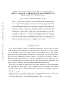
2 advantage of the performance of these architectures, the need for specific characteristics in new models/codes drove scientists from different fields to go back to the design board and start from scratch in the construction of their numerical algorithm. This is required by the need for very specific features that the numerical method must have to reach very high levels of scalability on the new machines. Most NWP codes in use today (at least in operational mode) are based on the finite-difference (FD) and spectral transform (ST) space discretization of the governing equations (see Tables 1.1-1.3). The ease of coding and their good performance have made FD popular with limited area models (LAM), whereas global circulation models (GCM) are mostly based on ST. In the era of high-performance computing, the search for efficient parallel codes on hundreds of thousands of processors is suggesting the implementation of alternative numerical methods that are based on local operation properties (element-based techniques). Of these, Galerkin methods (see Giraldo and Restelli (2008), Kelly and Giraldo (2012), or Dennis et al. (2012), among others) are the most common. The spectral element method (SEM) and discontinuous Galerkin (DG) are two examples. These alternatives are justified by the proven high parallel efficiency of local methods (Nair et al., 2011); their efficiency on large to very large machines is given by the minimal parallel communication footprint that is of vital importance as resolution increases. For a better understanding, let us make reference to Fig. 1.1, where two different computational grids are represented and compared against each other. In (a), the grid consists of nine finite elements Ωel h . Using element-based methods such as finite and spectral elements, the solution is sought on an element-by-element basis, making each element dependent on the others only through its shared boundary nodes. When the finite element grid is partitioned into smaller portions of the global domain, the only information that needs to be exchanged among the subdomains of the partition is that on the boundary nodes (or edges with DG) that each subdomain shares with its neighbors. In contrast, in (b) the grid is a classical structured, rectangular finite difference grid that here is plotted to be a direct analogue (in terms of node count) of the finite element mesh. Because a finite difference stencil is such that differentiation on each node in the domain requires information from a set of adjacent nodes (in the Cartesian directions only) that varies with the order of differentiation, when the domain is partitioned, certain specific nodes will belong to two overlapping subdomains. Because of this, a lot more communication is necessary. The belief that there is no possibility of efficient scaling with FD is false, if taken in an absolute sense. What may cause FD to lose efficiency in parallel is a combination of factors such as the order of differentiation or the number of nodes within each overlapping region. In the case of element-based schemes communication is naturally low by construction. The use of Galerkin methods in atmospheric simulations began five decades ago with the work on finite elements by Holmstrom (1963) and Simons (1968) in the 60s. This continued in the 70s (e.g. Cullen (1974), Francis (1972)) and was followed by an extensive production of articles in the 80s and 90s with, e.g., Staniforth (1984), Beland et al. (1983), or Burridge et al. (1986), who set the foundations of the operational Global Environmental Multiscale (GEM) model (Cote et al., 1998a; Yeh et al., 2002) of the

3

(a)

(b)

Figure 1.1: Examples of the adjacency pattern for a finite element Ωel h (a), and for a node that belongs to a finite difference grid (b). In (a) and (b) information is exchange, respectively, element- and node-wise. In (b), the only nodes that allow information to be shared between elements are the shared nodes on the boundary of neighboring elements (blue dotes on the boundary of Ωel h .). In (b), the cross made of blue circular nodes and a central red node is the stencil of a 2nd -order differentiation performed on the central node. How this plots relate to parallelization is described in the text.

Canadian Meteorological Center & Meteorological Research Branch (CMC-MRB). In the UK, Untch and Hortal (2004) used finite elements for the vertical discretization of a semi-Lagrangian transport scheme and introduced it in the operational version of the European Centre for Medium-Range Weather Forecasts (ECMWF) global spectral model (IFS), with great improvement with respect to the FD version of the code. At the same time, since Davies et al. (2006), the British Met Office committed to a FE approach for the treatment of the vertical atmosphere within their global and regional models. In the domain of Geophysical Fluid Dynamics (GFD), more Galerkin-type models appear since the beginning of the new millennium: in Brdar et al. (2012), Lauter et al. (2008), Nair et al. (2005), Giraldo and Rosmond (2004), Giraldo et al. (2002), and Giraldo (2000), different variational formulations mostly based on SEM and DG are employed to solve the shallow water equation, hyperbolic systems on the sphere, or the Navier-Stokes and Euler equations for non-hydrostatic problems on unstructured grids. Similarly, and with dynamic mesh adaptivity in mind, finite volume (FV) based softwares such as the German ICOsahedral Non-hydrostatic General Circulation Model (ICON) (Gassmann and Herzog, 2008; Bonaventura and Ringler, 2005), the Japanese Nonhydrostatic Icosahedral Atmospheric Model (NICAM) (Tomita and Satoh, 2004; Satoh et al., 2008), and the American Operational Multiscale Environmental model with Grid Adaptivity (OMEGA) by Bacon et al. (2000), are further examples of new trends in NWP. More recently, examples of element-based models are the SE/DG Nonhydrsotatic Unified Model for the Atmosphere (NUMA), whose linear scalability up to 32,000 cores for DG using MPI was shown in Kelly and Giraldo (2012), the SE Community Earth System Model (CESM) with scala-

4 bility shown up to 160,000 CPUs in Dennis et al. (2012), and DUNE (Brdar et al., 2012), a DG implementation of a finite element research code. Müller et al. (2011) are working on adaptive grid refinement and built an adaptive solver for atmospheric problems. In 2010, Aubry et al. (2010) presented their results from an edge-based finite element solver built on a fully unstructured grid. A descriptive list of existing research and operational models is reported in Section 1.2.

1.2

Existing models in NWP

Tables (1.1-1.3) report a non-exhaustive list of numerical models existing today in the atmospheric literature. The tables are organized by the type of spatial discretization that is used in each code. Ten out of the twenty-nine codes listed are based on the finite difference method. Except for the multiscale models Unified Model (UM), Nonhydrostatic Multiscale Model (NMMB), and EULerian LAGrangian (EULAG), all FD-based codes are limited area models (LAM). Spectral transform and finite volumes represent the second major trend (six codes each). Codes based on the spectral transform are common for GCM only. High-order element-based methods (spectral elements and DG) follow, while finite elements, only used in IFS (partially) and GEM, are the least common of all. For reasons that will become clearer in the chapters that follow, the temporal integration schemes that are mostly used are the split-explicit and the semi-implicit methods.

1.3

Aim of this thesis

Based on the consideration reported above on element-based methods, this thesis delves into the use of FEM and SEM to solve problems of typical interest in atmospheric simulations: (i) nonhydrsotatic, stratified, dry and moist flows, and (ii) transport in the atmosphere. Because of the instability that occurs in the numerical solution of (i) and (ii) (i.e., Euler and transport-diffusion equations), we stress the analysis on stabilization of FEM and SEM by the variational multiscale (VMS) scheme first introduced by Hughes (1995) and used extensively for incompressible flows and transport problems ever since. In this framework, this thesis has three main objectives. • Solution of the Euler equations using low-order finite elements stabilized by a compressible extension of VMS. Testing is performed using standard two- and three-dimensional benchmarks to verify the ability of this technique to solve compressible flows at low and very low Mach numbers. The algorithm is implemented within the multiphysics, multiscale, massively parallel code Alya2 . • Development of a variational multiscale stabilization scheme for high-order spectral elements to solve the advection-diffusion equation in atmospheric transport problems. Because monotonicity-preserving methods are particularly important in atmospheric transport, SEM + VMS is enhanced by a discontinuity capturing 2

Alya is developed at Barcelona Supercomputing Center, Spain. See Appendix B.

Model - Unified Model (UM)

Origin

Type

UK, Met. Office

NH

Fully compr. F D

LAM/GCM

semi-impl., semi-Lagrangian

NH

Fully compr. F D

(Malcolm, 1996) - COSMO

Germany, DWD

(Doms and Schattler, 2002) - WRF-ARW

LAM

split-expl. + semi-implicit

USA, NCAR and collaborations

NH

Fully compr. F D

LAM

semi-Impl., split Expl.

USA, NCEP and collaborations

HS/NH

Primitive eqns. F D

LAM

semi-Impl., split Expl.

NH

Primitive eqns. F D

LAM

leap frog

(Skamarock et al., 2007) - WRF-NMM (Janjic et al., 2001) - MM5

USA, NCAR and collaborations

(Dudhia, 1993) - Hirlam

France, Meteo France + coll.

(Room, 2001)

5

- MC2

Euler eqns. F D semi-Lagrangian, semi-impl.

USA, Colorado State U.

HS/NH

Primitive eqns. F D

LAM

leap frog


HS/NH

Primitive eqns. F D

LAM

semi Impl., split-expl


HS/NH

Primitive eqns. F D

LAM/GCM

semi Impl., split-expl

NH

Fully compr. F D

LAM

semi-impl., expl.

NH

Comprx./Incomprx. F D on generilized coords.

LAM/GCM

NFT (Non-oscil Forward in Time).

(Janjic, 1994) - NMM-B (Janjic, 2003) - COAMPS

USA, Naval Research Lab

(Hodur, 1997) - EULAG (Prusa et al., 2008)

Primitive eqns. F D semi-Impl., semi-Lagrangian (vert.)

NH

(Pielke et al., 1992) - ETA

NH LAM LAM

Canada, Res. Centr. for NWP

(Benoit et al., 1997) - RAMS

Equations and Numerical Scheme

USA, NCAR

Table 1.1: Existing atmospheric models in NWP

UK, ECMWF

(Untch and Hortal, 2004) - CAM EUL

USA, NCAR

(Neale et al., 2010) - NOGAPS (until 1998)

semi-Impl.

GCM

cetranl time-diff.+ semi-impl. corr.

France, Meteo France

HS/NH

Fully compr. ST + F D in z

LAM


European consortium

www.cnrm.meteo.fr/arome/ Germany, DWD

(Majewski et al., 2002) - OMEGA

USA, Centr. Atmo. Phys.

(Bacon et al., 2000) - ICON

(Satoh et al., 2008) - CAM FV

(Ullrich et al., 2010)

Primitive eqns. ST (split-expl) semi Impl.

NH

As ALADIN-NH+soph. physics ST

LAM

semi-impl.

NH

Primitive eqns. F V /SE

GCM

semi-implicit

NH

Fully compr. F V

GCM

split-expl, semi-impl.

NH

Fully compr. F V

GCM

semi-implicit

Japan

NH, GCM

Euler Eqns. F V

Agency for Marine-Earth Science

LAM

split-expl, semi-impl.

USA, NCAR

(Neale et al., 2010) - MCore

HS/NH LAM/GCM

Germany, MPIfM + DWD.

(Gassmann and Herzog, 2008) - NICAM

shallow atmo., ST + F D in z Primitive eqns. ST

France, Meteo France

- GME

semi-Impl., semi-Lagrangian.

HS NH

(Courtier et al., 1991) - AROME

LAM GCM

(Laprise, 1992) - ARPEGE

Fully compr.+ T, ST + F E in z


(Hogan et al., 1991) - ALADIN-NH

NH

USA, U. Mich.

HS

primitive eqns. F V

GCM

Explicit

NH

Fully compr. F V

GCM Table 1.2: Existing atmospheric models in NWP. (Continuation of Tab.1.1).

6

- IFS

- NUMA

USA, Naval Postgraduate School

(Kelly and Giraldo, 2012) - DUNE

Germany, U. Freiburg

(Brdar et al., 2012) - NSEAM (from NOGAPS)


7

(Giraldo and Rosmond, 2004) - HOMME

USA, NCAR

(Thomas and Loft, 2005) - GEM (Cote et al., 1998b)

Canada, CMC & MRB

NH

Fully compr. SE/DG

unified: LAM/GCM

Implicit/Explicit (IMEX)

NH

Fully compr. DG

unified: LAM

Expl. (other options)

NH

Primitive eqns. SE

GCM


HS

Primitive eqns. SE

GCM

Explicit + other options

HS+NH

Primitive eqns., F E

LAM/GCM

semi-Lagrangian, impl.

Table 1.3: Existing atmospheric models in NWP (Continuation of Tab.1.1)

8 scheme to approach a quasi-monotonic solution. The algorithm is developed within the massively parallel, multiscale, atmospheric code NUMA3 . • To close the circle of applications, the Euler and transport equations are coupled to model the flow of moist atmospheres where warm, precipitating clouds form. This represents a proof-of-concept of the ability of Galerkin methods stabilized by VMS to solve problems of atmospheric relevance. To achieve this goal, the low-order finite elements that define the first objective of this study are extended to coupled problems with complex physics. To our knowledge, the FEM and SEM algorithms with VMS proposed in this thesis represent the first continuous Galerkin methods with VMS stabilization applied to problems that are important for atmospheric modelers.

1.3.1

Publications derived from this work

Based on this work, the following publications were derived: three peer-reviewed research papers, two short conference articles, one technical report, and a set of talks given in international conferences and workshops. Peer-reviewed journal articles • Marras, S., Kelly, J. F., Giraldo, F. X., and Vázquez, M. 2012. “Variational Multiscale Stabilization of High-Order Spectral Elements for the Advection-Diffusion Equation” Journal of Computational Physics 231, 7187-7213. • Marras, S. Moragues, M. Vázquez, M. Jorba, O., and Houzeaux, G. “A Variational Multiscale Stabilized Finite Element Method for the Solution of the Euler Equations of Nonhydrostatic Stratified Flows”, Journal of Computational Physics (To appear. DOI: 10.1016/j.jcp.2012.10.056). • Marras, S. Moragues, M. Vázquez, M. Jorba, O., and Houzeaux, G., “A Variational Multiscale Stabilized Finite Element Method for the Solution of the Euler Equations of Moist Atmospheric Flows”, Journal of Computational Physics (Submitted, July 2012). In proceedings • Marras, S., Vázquez, M. Jorba, O. Aubry, R., and Houzeaux, G. 2010 “Application of a Galerkin Finite Element Scheme to Atmospheric Buoyant and Gravity Driven Flows” AIAA paper 0690, p. 7860-7869. In Proceedings of the 48th AIAA 3

NUMA is developed at the department of Applied Mathematics at the Naval Postgraduate School, U.S.A. See Appendix B.

9 Aerospace Sciences Meeting Vol. 9, ISBN: 978-1-61738-422-6, Curran Associates, Inc. • Aubry, R., Vázquez, M., Houzeaux, G., Cela, J. M., and Marras, S. 2010 “An Unstructured CFD Approach for Numerical Weather Prediction” AIAA paper 0691, p. 7870-7895. In Proceedings of the 48th AIAA Aerospace Sciences Meeting Vol. 9, ISBN: 978-1-61738-422-6, Curran Associates, Inc. Talks at conferences and workshops • Marras, S. 2012 "Stable and quasi-Monotonic SEM Solutions using Variational Multiscale Stabilization", Newton Institute for Mathematical Sciences, Cambridge University (UK). Oct. 16, 2012. • Marras, S. 2012 "3D Simulations of Convective Storms using Finite Elements with Variational Multiscale Stabilization", Newton Institute for Mathematical Sciences, Cambridge University (UK). Nov. 22, 2012. • Marras, S., Kelly, J. F., and Giraldo, F. X. 2011“Towards Positive High-Order Spectral Elements for the Advection Equation”, Institute for Pure and Applied Mathematics (IPAM), UCLA, U.S.A., Reunion meeting. Lake Arrowhead, December. • Marras, S., Vázquez, M., Jorba, O., Houzeaux, G., and Folch, A. 2010, “Solving Nonhydrostatic Dynamics with a Variational Multiscale Galerkin Solver: Tests and Parallel Performance”, Institute for Pure and Applied Mathematics (IPAM), UCLA, U.S.A. (2010) Long program Model and Data Hierarchies for Simulating and Understanding Climate, Los Angeles, March 2010 - June 2010. • Vázquez, M., Marras, S., Moragues, M., Jorba, O., Houzeaux, G., and Aubry, R. 2010, “A Massively Parallel Variational Multiscale FEM Scheme Applied to Nonhydrostatic Atmospheric Dynamics”, EGU Annual Meeting, EGU-2010-9060, Vienna, Austria

1.4

Organization of the manuscript

The remainder of this thesis is organized as follows. Chapter 2 presents a brief introduction to the physical problem of atmospheric dynamics and its mathematical modeling. It is followed by a general description of the finite and spectral element methods with a brief overview to the issues related to their stabilization. Chapter 4 reports on the application of finite elements and variational multiscale stabilization for the solution of the fully compressible Euler equations. Chapter 5 shows the solution of the advection-diffusion equation by means of high-order spectral elements. The main issue of monotonicitypreserving high-order methods is covered as well. The solution of moist atmospheres with phase change is described in Chapter 6. Conclusions are presented in Chapter 7.

10 Appendix A presents some CFD grid generation techniques that can be of practical use in atmospheric modeling. The two computational environments are presented in Appendix B. The relationship between the equation of θ and T is reported in Appendix C.

Chapter 2

The physical problem The best world has the greatest variety of phenomena regulated by the simplest laws –Gottfried W. Leibniz, c. 1700 In this chapter we present the set of equations that govern atmospheric dynamics and transport phenomena in the atmosphere. We discuss the different formulations and justify the selection of the set that is used throughout this thesis.

2.1

Dynamics of dry atmospheres

The motion of the earth atmosphere can be described by the laws of fluid mechanics under the assumption that the air is treated as a continuum. As such, the state of the gas can be described by density, ρ, pressure, p, absolute temperature, T , and a velocity field, u (Ockendon and Ockendon, 2004). At given T , u, and height h, the total energy e of the fluid flow is given by the contribution of internal energy ei = cv T , kinetic energy ek = (u · u)/2, and potential energy Φ = g h, where cv is the gas heat coefficient at constant volume and g = 9.81 m s−2 is the modulus of the acceleration of gravity. From the principles of conservation of mass, momentum, and energy, the Navier-Stokes equations of fluid dynamics are a proper set to describe atmospheric motion. Subgrid viscous effects in atmospheric simulations are typically introduced through the subgridscale eddy viscosity of turbulence. Since eddy viscosity is much larger than molecular viscosity, the effects of molecular viscosity in mesoscale models are typically neglected. In this thesis, however, turbulence effects will not be considered and the Euler equations will be used as a suitable model for the problems described throughout. Nor will we consider the forces due to Coriolis1 because of the relatively small scales of interest considered throughout. Viscous effects in modeling the atmosphere are indeed 1

For the time being, the hypothesis of a non-rotating domain is considered. In fact, the main goal of this work is not that of modeling a real weather problem, in which case, it is likely that Coriolis effects cannot be neglected, but rather testing a numerical algorithm to verify its suitability for non-hydrostatic stratified simulations in idealized conditions.

11

12 introduced when needed, but this is achieved through the use of proper turbulence closures. The problems treated in this thesis are sufficiently idealized that inclusion of turbulence is not necessary. The governing equations of interest are described in what follows. Let x = (x, z) and x = (x, y, z) be a Cartesian, fixed frame of reference of dimensions d = 2, 3 and let t ∈ R+ be the time variable. Assuming that ρ is a non-negative function of x and t, mass conservation can be expressed by the conservation law ∂ρ + ∇ · U = 0, ∂t

(2.1)

where ∇· is the divergence operator acting upon momentum U = ρu. U has components (U, W )T and (U, V, W )T in two and three dimensions, respectively. Conservation of U for a non-viscous fluid reads

∂U U⊗U +∇· + Ip = − gez ρ, ∂t ρ

(2.2)

where I and ⊗ are the identity tensor and tensor product, respectively, and ez is the unit vector directed along the vertical direction (z). In the case of an incompressible flow, the conservation of mass reduces to ∇ · u = 0 and the system of Eqs. (2.1)-(2.2) is self-contained. This is truepwhen the flow Mach number M = kuk2 /c is smaller than 0.3 approximately (c = ∂p/∂ρ is the speed of sound). Otherwise, compressibility effects become important in that a variation of pressure implies a variation of density and temperature. A constitutive equation is needed to express the relationship among the three thermodynamics variables. The variation in temperature is modeled by the additional equation of conservation of total energy: ∂ρ e + ∇ · [(ρ e + p) u] = 0. ∂t

(2.3)

At present, only a few atmospheric models are based on Eqs. 2.1-2.3. This set is at the base of the global, icosahedral, nonhydrostatic model for global cloud resolving simulations (NICAM) described by Tomita and Satoh (2004) and Satoh et al. (2008), and was compared against other sets by Giraldo and Restelli (2008).

2.2

Approximations and sets of common use in atmospheric simulations

By algebraic manipulation and/or suitable approximations, the Euler equations are often re-expressed by alternative formulations as a way, for example, to filter motions and solutions that are of no interest for the problem being considered (e.g., sound waves) (Thuburn, 2011a), or to inherently find a direct link between the physics and the set of

13 variables that describes it. In this respect, each set has its advantages and drawbacks. Unquestionably, no set is optimal per se; it is optimal within a very specific context that, in the case of atmospheric simulations, is not unique. For example, let us introduce the Exner function π = (p/p0 )R/cp , a normalized pressure given a reference base-state pressure p0 , and the relation between π and potential temperature as θ = T /π. A change of variables from ρ, p, and e to π and θ yields the self-contained system R ∂π + u · ∇π − π∇ · u = 0, ∂t cv

(2.4a)

∂u + u · ∇u + cp θ∇π = −gez , ∂t

(2.4b)

∂θ + u · ∇θ = 0, ∂t

(2.4c)

where (π, u, θ)T is the vector of the solution variables (Durran, 1998; Cullen, 1990). The advantage is clear: the system of (2+d) equations only has (2+d) unknowns so that there is no need for an extra equation to close the system (e.g., equation of state). Not only that, but the use of θ rather than energy is advantageous, in terms of the physics, because information on the stability of the atmosphere is given by ∂θ/∂z (Restelli, 2007; Smith, 1979). Of the most common models that use this formulation we list MM5 developed at Penn State and NCAR (Dudhia, 1993), NMM based on the work by Janjic (2003) at NCEP, COAMPS (Hodur, 1997) developed at the U.S. Naval Res. Lab., and HIRLAM (Room, 2001, 2002) by a consortium of European Numerical Weather Services. Another set of common use is given by the conservation laws of (ρ, U, Θ)T (T indicates the vector’s transpose): ∂ρ +∇·U=0 ∂t

(2.5a)

∂U U⊗U +∇· + pI = −ρgez ∂t ρ

(2.5b)

(2.5c)

∂Θ ΘU +∇· =0 ∂t ρ where Θ = ρθ is density potential temperature. The state law for pressure p = p0

RΘ p0

γ

(2.6)

completes the system. γ = cp /cv , where cp and cv are the heat coefficients at constant pressure and volume, respectively.

14 The ARW-WRF model (Skamarock et al., 2007) is based on this set, and so are the finite volume simulations by Ahmad and Lindeman (2007), the UK Meteorological Office Unified Model (UM) (Jackson et al., 2001; Malcolm, 1996), and the German LM model (COSMO, 1998). Finally, computational efficiency suggested the use of the following set in research codes such as the Nonhydrostatic Unified Model for the Atmosphere (NUMA) developed at the Naval Postgraduate School (Kelly and Giraldo, 2012): ∂ρ + ∇ · (ρu) = 0, ∂t

(2.7a)

1 ∂u + u · ∇u + ∇pI = −gez , ∂t ρ

(2.7b)

∂θ + u · ∇θ = 0, ∂t

(2.7c)

plus equation (2.6).

2.2.1

Remarks on the equation of total energy

The conservation equation of total energy can be replaced by the equation of transport of total temperature. The two equations are mathematically equivalent. However, in the presence of strong pressure waves (i.e. shocks), the numerical solution of the T equation places the discontinuity in the wrong position. Clearly, in the case of atmospheric flows there are no shocks to worry about, so that equation 1 ∂T = −u · ∇T + p∇ · u ∂t cv ρ

(2.8)

is equivalent to Eq. (2.3). Because atmospheric stability is directly linked to the variation of θ along z, in atmospheric simulations the use of θ is advantageous over the use of T or E. For this reason, all but one set described above express energy in terms of potential temperature. One way to see the equivalence is reported in Appendix C. Due to practical reasons related to the stabilization scheme (See Chapter 4 below), the set of equations used in this thesis is composed by the continuity and momentum equations of set (2.5), and by Eq. (2.7c). ρ, θ, and p are related by (2.6). In summary, we are interested in the system ∂ρ + ∇ · U = 0, ∂t

U⊗U ∂U +∇· + pI = −ρgez , ∂t ρ

(2.9a)

(2.9b)

15

∂θ U + · ∇θ = 0. ∂t ρ

(2.9c)

For how linearization is constructed (see page 37), we express ∇p with respect to ρ and θ. From the state equation p = c0 (ρθ)γ , where c0 = Rγ /pγ−1 , we have that 0 ∇p = c0 γ(ρθ)γ−1 [ρ∇θ + θ∇ρ] . What has been stated so far applies to dry environments only. The necessary corrections, definitions, and derivations for a moist atmosphere will be given in Chaper 6.

2.2.2

Nearly-hydrostatic flows

Dynamics in the atmosphere is characterized by small variations of the thermodynamic quantities with respect to some background reference state (Marchuk, 1974; Klein, 2000). This is expressed by the splitting ρ(x, t) = ρ′ (x, t) + ρ¯(z), p(x, t) = p′ (x, t) + p¯(z), and ¯ θ(x, t) = θ ′ (x, t) + θ(z), where the primed and barred quantities represent, respectively, the perturbation and the background state of ρ, p, and θ. They are such that ρ′ ≪ ρ¯, ¯ When vertical acceleration is zero, the vertical component of Eq. p′ ≪ p¯ and θ ′ ≪ θ. (2.9b) simplifies to the equation of hydrostatic balance ∂z p¯ = −gρ¯.

(2.10)

Given these considerations and the analysis of nearly-hydrostatic flows for well-balanced methods (Botta et al., 2004), set (2.9) changes to ∂ρ +∇·U=0 ∂t

(2.11a)

∂U U⊗U +∇· + p′ I = −ρ′ gez ∂t ρ

(2.11b)

∂θ U + · ∇θ = 0 ∂t ρ

(2.11c)

System (2.11) is used in this thesis.

2.3

Hydrostatic vs nonhydrostatic models

Atmospheric models can be distinguished as hydrostatic and non-hydrostatic. If we assume the vertical acceleration to be negligible, the vertical momentum equation of the hydrostatic system reduces to the diagnostic equilibrium equation (2.10). At every timestep, this time-independent equation is solved instead of the full equation for vertical

16 momentum. Sound waves in the vertical direction are eliminated (Durran, 1998). They are not, however, eliminated in the horizontal direction. Because the size of the domain in the horizontal direction is typically much larger than the vertical depth of the atmosphere, and the grid size along x and y may be orders of magnitude larger than the grid spacing along z, the stiffness of the problem in the sense of grid size and corresponding time-step size is relaxed. The hydrostatic approximation has been the core of NWP for the past four decades. This approximation is valid for horizontal grid spacing larger than 10 km (Janjic, 1994; Thuburn, 2011a). The hydrostatic approximation is still appropriate to simulate synoptic scale phenomena where the vertical acceleration can be neglected, but is no longer considered in any mesoscale simulation. With the availability of more powerful computers, nonhydrostatic formulations have eventually been investigated (see, Janjic et al. (2001); Benoit et al. (1997); Bonaventura (2000); Gassmann (2005); Grell et al. (1995); Hodur (1997); Janjic (2003); Skamarock et al. (2007); Xue et al. (2000); Giraldo and Restelli (2008)) and are today the rule in the numerical approximation of mesoscale dynamics.

2.4

Transport in the atmopshere

In this thesis, the governing equations of a dry atmosphere are coupled to a set of transport equations for tracers (see Chapter 6). Generally speaking, a tracer is any quantity that is transported by the flow. This includes water species, chemicals, aerosols, and others. Their transport is described by the same equations. As for the case of Eq. (2.1), conservation of mass for a tracer i of density ρi and mixing ratio qi = ρi /ρ is expressed by ∂ρ qi = −∇ · (ρ qi u) + Si , ∂t

(2.12)

where Si represents sources or sinks and where, for simplicity, diffusion is neglected. For example, in the case of water vapor, Si is driven by evaporation and condensation. In spite of the mathematical simplicity of Eq. (2.12), its correct numerical approximation is still an open field of research. The importance of its correct numerical representation is vital in NWP. To understand this we introduce the concept of tracer-air mass consistency (see, Lauritzen et al. (2011) and references therein). In the case of the continuous equations, if qi = 1 Eq. (2.12) reduces to the equation of conservation of air. In discrete space, this is certainly not achieved if the equation of conservation of air mass and of the tracer are solved by two different numerical methods. This is a classical issue in the case of either online applications that use different numerics for different equations (e.g., transport of reacting chemicals vs transport of dry air), and even more so in the case of offline simulations where the air mass properties come from a different model or observations. Although this topic is not treated in this thesis, we believe that it is worthwhile to keep this in mind throughout the development of a new atmospheric model, such as the case of the one described below. To conclude this introduction to the physical problem, we write the advective form of

17 (2.12) that will be used later on. We are aware of the inconvenient properties (e.g., conservation) that this form carries (Lauritzen et al., 2011). Nevertheless, it is a classical formulation of the equation of transport of water concentration (water vapor, cloud water, rain, ice, etc.) that is used in weather forecasting. By using the equation of mass of dry air to eliminate ρ from (2.12), we obtain: ∂qi = −u · ∇ qi + Si . ∂t

(2.13)

This is not the equation of conservation of qi . Moreover, no numerical method of solution will be conservative on (2.13). We will touch more on this in Chapter 5. As moisture is an extremely noisy variable that could cause serious stability and convergence problems, the capacity of a numerical scheme to produce a monotonic solution to (2.13) is another relevant point to analyze. If, for example, our system produced negative moisture, the physical parametrization would have to resolve this issue in some way (e.g. filtering the negative values); the wrong feedback that this condition will send to many other variables would, in turn, affect the moisture and hence cause artificial rain to be produced. The words of John P. Boyd are an amusing conclusion to this paragraph: "[...] Clever adaptive algorithms that work for smooth, straight shocks disintegrate into computational anarchy when flayed by gravity waves, assaulted by moist convective instability, battered by highly temperature-sensitive photochemistry, and coupled to the vastly different time and space scales of the ocean[...]" (SIAM News, Multiscale Numerical Algorithms for Weather Forecasting and Climate Modeling: Challenges and Controversies. Nov 2008, Vol.41 issue 9). Monotonic solutions are certainly more difficult to achieve with high order numerical methods. The problem is particularly challenging when Eq. (2.13) is solved by the spectral element method. In Chapter 5 we will specifically address this problem.

2.5

Characteristic scales in dynamic meteorology

Since the work by Ligda (1951) on radar observations of storms, atmospheric motions have been categorized into three spatial scales as follows: microscale: l < 20 km, mesoscale: 20 km < L < 1000 km, and synoptic scale: L > 1000 km. A similar subdivision comes from Pielke (2002), but according to whom mesoscales only extend from 20 to 200 km, leaving a larger synoptic range (> 200, km). Earlier on, Stull (1988) called macro what is synoptic to Pielke, defined mesoscale the range between 200 m and 200 km, and assigned micro and microδ the ranges 2 m−10 km and 0−2 m respectively. Further scales were defined as macro-α (L > 10000 km), macro-β (10000 km > L > 2000 km), meso-α (2000 km > L > 200 km), meso-β (200 km > L > 20 km), meso-γ (20 km > L > 2 km), micro-α (2 km > L > 200 m), micro-β (200 m > L > 20 m) and micro-γ (L < 20 m) by Orlanski (1975), and based on other observations, atmospheric phenomena have also been categorized into masoscale, mesoscale, misoscale, mososcale and musoscale by Fujita (1981).

18 Table (2.1) lists the main characteristic scales of interest. The difference between global, synoptic, meso, and urban (L < 200 m) is relevant when looking at the terms to be considered in the equations, and consequently when deciding on the numerical solution. In the case of the work that we present, the equations and the numerical method apply to problems in mesoscale meteorology. The finite element method in itself is not scale-selective; this means that a finite element-based dynamical core, after proper modification of the equations (i.e., additional Coriolis effects), could, in theory, be transferred onto the global/synoptic scale in a unified manner as reported in the recent work by Kelly and Giraldo (2012). This will not be treated, but it is a great advantage to consider for it lies at the basis of the global extension of the algorithm to global scales.

2.6

Summary

In this chapter, we described the different sets of equations that are commonly adopted in atmospheric modeling. Of these, we focused on different formulations of the Euler equations in stratified environments and defined the equations that will be used in this thesis (set 2.11). Leaving the details for a dedicated part of the document (Chapter 6), we also introduced the transport equations of passive tracers that describe advection of water tracers in the atmosphere (Eq. (2.13)). No further details were given on the coupling of the two systems because it would require explanations that, at this point along the manuscript, may result unclear to the reader who is not familiar with wet atmospheric dynamics. The material that was presented is sufficient to introduce part of the notation and the framework within which the thesis is developed. Certain topics of equal weight in NWP, such as the construction of the anelastic and pseudo-incompressible equations to filter acoustic waves (see, e.g., Durran (2008) and references therein), or the shallow-water equations fall beyond the scope of this thesis.

19

Table 2.1: Scales of atmospheric motions. Adapted from page 5 of Holton (2004), and from Fig. 1.1 of Thuburn (2011a)

Type of motion

Horizontal scale (m)

Time scale (s)

10−2 -102

10-108

10−2 − 10−1

101

10−1 − 1

101

1 - 10

101

10 - 102

101 -102

Tornadoes

102

103

Cumulonimbus clouds

103

103 -104

104 − 105

104

Hurricanes

105

105

Synoptic cyclones

106

105 -106

Planetary waves

107

106

Molecular diffusion Minute turbulent eddies Small eddies Dust devils Gusts

Fronts, squall lines

20

Chapter 3

Numerical methods: Finite and Spectral Elements It is necessary to solve differential equations –Isaac Newton, c. 1700 In this chapter, the fundamentals of the approximation of partial differential equations (PDEs) by Galerkin methods are introduced. The finite element and the spectral element methods, FEM and SEM respectively, are a special type of Galerkin approximation techniques. We introduce the ideas behind Galerkin schemes in general and then distinguish between FEM and SEM in particular. We define their properties and underline the most salient differences. The FEM solution of a 1D steady-state, scalar, linear, advection-diffusion (AD) equation is then used to present the idea of unbounded solutions and the need for numerical stabilization. Finally, we introduce the fundamentals of a particular category of stabilization techniques in the context of Galerkin methods to familiarize with one of the numerical contents used in the chapters that follow.

3.1

Galerkin methods

Introduced in the early 40s in the study of vibration and equilibrium (Courant, 1943), but extensively developed only in the late 1950s by structural dynamicists in the aircraft industry, finite element methods1 are among the most common numerical methods in use today in a wide range of applications (e.g. structural analysis and design (Yang, 1985), fluid dynamics (Zienkiewicz et al., 2005), electromagnetism (Bastos and Sadowski, 2003). Accepted by scientists and engineers in theoretical studies and applications, the ease in modeling complex geometries, the flexible and general purpose programming format that it implies, and the intrinsic treatment of differential-type boundary conditions made it a robust tool for the solution of any differential problem (Donea and Huerta, 2003). 1

Spectral elements are finite elements as well. The difference, that will result clear by reading this chapter, lies in the type of element that is used in the sense of approximation.

21

22 In the following, we will deal with the idea behind the method of weighted residuals, of which the Galerkin finite and spectral element methods represent a special case. For a simple but quasi-rigorous analysis of the method we use a problem of real engineering interest and that, as we presented in Chapter 2, is a fundamental problem in numerical weather prediction: the advection-diffusion equation. The reader is referred to the books by Fletcher (1987), Quarteroni and Valli (1994), and Karniadakis and Sherwin (1999) as a reference for the more mathematical aspects of Galerkin methods. Let us take a general differential problem L(q) = f,

(3.1)

where L is the combination of differential operators in space x and time t, and f is a forcing function. Let d indicate the space dimension and let Ω ⊂ Rd be the domain bounded by the boundary ∂Ω where (3.1) is defined within the time interval (0, tf ), and t f ∈ R+ . For the problem to be well-posed, suitable boundary and initial conditions must be added to (3.1). Unless otherwise stated, given a known function g, Dirichlet boundary conditions q(x) = g for x ∈ ∂Ω will be applied to the problems described throughout this work. As previously said, Galerkin methods are a particular case of the method of weighted residuals. The idea behind this method is the numerical representation of the solution variable q by a finite dimensional approximation q h obtained by the expansion q h (x) =

N X

ψk (x) qˆk ,

(3.2)

k=0

where N is the number of k nodes pk of a possible partition of the continuous physical domain Ω. On its discrete counterpart, Ωh , a set of k = 0, . . . , N known analytic test functions ψk are defined (The two terms test and basis will be used interchangeably. Basis comes from the properties of ψ in the context of function spaces). The unknown coefficients qˆk correspond to the physical values of q at node pk . The finite difference method is conceptually different in that what is approximated in the differential problem are the differential operators and not the solution variable. Substitution of (3.2) into (3.1) is such that L(q h ) − f 6= 0. The method is called method of weighted residuals because a linear system of algebraic equations in the unknowns qˆ is built by imposing that Z

w R dΩ = 0,

(3.3)

Ω

where R = L − f is the residual of (3.1) and w is the weight function that has certain properties. Different methods arise from the selection of different w. The Galerkin

23 method is found when w = ψk . We can then write the following: Z

Ω

ψ [L − f ] dΩ = 0,

(3.4)

This is the weak form of the original equation to be solved. Remark 3.1. So far, no distinction between the finite and spectral element methods has been made. The difference stems from the definition of ψk and will be reported shortly.

3.1.1

Suitable function spaces

Not every basis function ψ is accepted for the Galerkin formulation of a differential problem to make sense. In the specific cases of the advection-diffusion equation and the Euler equations of compressible flows, the highest order of derivation is 2, and the choice of the basis functions and the space to which they belong must depend on this regularity condition. The first step to take in the construction of the Galerkin method after defining the weak form of the original differential equation (e.g. Eq. (3.4)) is integration by parts to eliminate the second derivatives and hence impose a lower regularity on the solution . variable (Quarteroni, 2009). In the simple case where L(q) = ∇ · (ν∇q) = 0 is the Laplace equation for diffusion of q in a medium with diffusivity ν, integration by parts is such that Z

Ω

ψ ∇ · (ν∇q) dΩ = −

Z

Ω

ν∇ψ · ∇q dΩ,

(3.5)

where the assumption ψ(∂Ω) = 0 was used given Dirichlet boundary conditions on q. To understand under what conditions the integral on the right-hand side of Eq. (3.5) is defined, we first need to define the space of functions v that are Lebesgue integrable up to power p = 1, . . . , ∞ as: . Lp (Ω) = {v : Ω → R s.t.

kvkLp = Ω

Z

Ω

|v|p dΩ

1

p

< ∞}.

(3.6)

We also need to refer to the Cauchy-Schwarz inequality according to which, given two functions u, v ∈ L2 , we have that Z

Ω

|uv| dΩ ≤ kukL2 kvkL2 .

(3.7)

It was stated within the definition of Lp that all the norms k · kLp are bounded. (3.6) R and (3.7) simply imply the boundedness of Ω |uv| dΩ, which is equivalent to saying that uv ∈ L1 (Ω). These steps are a very simple analysis of the least regularity requirement for the product ∇ψ · ∇q. This requirement is fulfilled if u = ∇q and v = ∇ψ belong

24 to L2 (Ω). This means that we need to define a space where not only the functions, but their first derivatives are square integrable as well. We define: . H 1 (Ω) = {v ∈ L2 (Ω) H1

∂v ∈ L2 , j = 1, . . . , d}. ∂xj

s.t.

(3.8)

The space W of test functions ψ and trial solutions q of problem (3.4), is a subset of such that . W = {ψ, q ∈ H 1 (Ω) s.t.

ψ = 0 and q = g on ∂Ω}.

(3.9)

The previous analysis is far from being exhaustive but more of it would fall beyond the scope of this work. Nevertheless, the basic definitions reported so far are necessary to set the foundations of the Galerkin methods that will be used throughout.

3.1.2

Finite and Spectral Elements: discretization and basis functions

To discretize the problem in a finite and spectral element sense, the domain Ω is first decomposed into a finite element partition P h = {K i }iel=1,...,nel of nel conforming2 elements K i such that Ω=

n el [

K i,

iel=1

and

n el \

K i = 0,

(3.10)

iel=1

where every element K i is the image of the reference element I = [−1, 1]d by a nonsingular bijective mapping x = Hi (ξ) from physical space x to computational space ξ. J = dx/dξ is the transformation Jacobian matrix. A two-dimensional example of mapping is represented in Fig. 3.1. The need for mapping is purely practical and forms the foundations of finite element computation. For details see Hughes (2000). Basis functions: Finite Elements. Due to the properties of Lagrange polynomials, Lagrange basis functions are a common choice in finite elements. These functions, defined by hk from now on, have the property of being piecewise continuous and are such that hk (xl ) = δkl

k, l = 0, . . . , N,

where δkl is the Kronecker delta. In the case of linear Lagrange polynomials, this translates into piecewise linear functions. This applies for any space dimension. The basis functions, in practice, are constructed only once on the reference element. At the moment of computing the integrals by a suitable quadrature rule, the mapping to physical space is computed. 2

Being conforming is not a requirement as far as the construction of Galerkin methods goes. It is, however, a constraint if the code cannot treat hanging nodes.

25

Figure 3.1: Mapping from reference, (ξ, η), to physical space, (x, z). ∀K i ∈ P h :

K i = Hi (I).

For linear, quadratic, and cubic finite elements, the roots of the basis function along the reference element I are the N+1 equi-spaced nodes within the element. Using the definition of the Lagrange polynomials hk (ξ) =

N Y

ξ − ξl , ξ − ξl l=0,l6=k k

(3.11)

in Fig. 3.2 we plot hk along a reference element up to 2nd -order. A 4th -order finite element and corresponding basis function are plotted in Fig. 3.3 (left).

Basis functions: Spectral Elements. Unlike the case of high-order finite elements, the polynomials used with spectral elements are associated with zeros that are not equispaced. A classical and convenient set is represented by the Legendre-Gauss-Lobatto (LGL) points. LGL nodes ξi are the roots of (1 − ξ 2 )PN′ (ξ) = 0,

(3.12)

being Pn (ξ) the Nth -order Legendre polynomial whose construction by recursive formulas can be found in Karniadakis and Sherwin (1999). The polynomials that are used have the same δ-property of the Lagrange polynomials defined above. Their analytic expression is given by hk (ξ) =

(ξ 2 − 1)PN′ (ξ) , N (N + 1)(ξ − ξk )PN (ξ)

k = 0, . . . , N,

(3.13)

where P ′ indicates derivation with respect to x. The 4th -order k-polynomials along I = [−1, 1] are plotted on the right panel of Fig. 3.3. The comparative plot (finite

26 1st order Lagrange Basis Functions

2nd order Lagrange Basis Functions

0.5

0.5

h(x)

1.0

h(x)

1.0

0.0

0.0

-0.5

-0.5

-1.0 -1

-0.5

0

x

0.5

1

-1.0 -1

-0.5

0

x

0.5

1

Figure 3.2: Lagrange polynomials of order 1 (left) and 2 (right) along the 1D reference element I = [−1, 1]. Clearly, they are equivalent for FE and SE.

element on the left and spectral element on the right) is used to show that, if highorder is required, equi-spaced nodes produce unsatisfactory types of basis functions in the proximity of the edge points of the element. In other words, we lose control on the maximum and minimum values of hk at the extrema of the element. When this happens, interpolation of any function is likely to suffer from such condition. To show how this feature translates into the interpolation of a known analytic function, we use the following example from Giraldo (2011). We define the Witch of Agnesi of unitary height as z(x) =

1 , 1.0 + 50 x2

where z(x) is smooth and continuous, and interpolate it using the basis functions ψ(x) = hk (x) defined above. The test is performed by 4th -order interpolation. Equi-spaced and non equi-spaced points are used along the unitary domain. Fig. 3.4 shows how, the more the polynomial order is increased, and the better the result is when LGL nodes are employed. Roughly speaking, this analysis serves as a practical way of showing one reason for the use of LGL points in high-order simulations rather than high-order elements with evenly distributed nodes. Figure 3.5 is a schematic representation of two 4th -order elements in two dimensions.

3.2

Galerkin method and unbounded solutions

The straight numerical approximation of problems with dominating advection may result in unphysical oscillations in the solution. Galerkin methods represent no exception

27

4th order Lagrange Basis Functions

4th order Lagrange Basis Functions

0.5

0.5

h(x)

1.0

h(x)

1.0

0.0

0.0

-0.5

-0.5

-1.0 -1

-0.5

0

0.5

x

-1.0 -1

1

-0.5

0

0.5

x

1

Figure 3.3: Basis of order 4 along the 1D reference element I = [−1, 1]. Left: the nodes within the element are equi-spaced as for classical high-order FE. Right: Lagrange-Legendre polynomials of order 4 whose roots are the non-equi-spaced Legendre-Gauss-Lobatto (LGL) quadrature points. Nodal SE and DG may employ LGL or LG quadrature. However, to obtain a diagonal mass matrix then LGL is the only choice for SE, while LG can still be used for DG.

1.0

4th-order Interpolated vs Exact Solution q

0.8

Equisp. q

3.5

10th-order Interpolated vs Exact Solution

e

q

3.0

h

Equisp. q

h

e

h

h

LGL q

LGL q

2.5

0.6

2.0

qh, qe

qh, qe

0.4 0.2

1.5 1.0

0.0 0.5 -0.2

0.0

-0.4 -0.6 -1

-0.5 -0.5

0

x

0.5

1

-1.0 -1

-0.5

0

x

0.5

1

Figure 3.4: Interpolation of a known function (Witch of Agnesi) using high-order interpolating functions with equi-spaced and LGL points. Left: 4th -order interpolation. Right: 10th -order interpolation

28

Figure 3.5: Nodes disposition for a two-dimensional 4th -order finite element (left), and spectral element (right).

(Johnson et al., 1984). An error estimate of the standard Galerkin approximation of the problem proves it (see, e.g., Quarteroni and Valli (1994)). Here, we show it by working out the 1D finite element solution of the advection-diffusion problem with Dirichlet boundary conditions. The problem is that of solving . L(q) = u · ∇q − ∇ · (ν∇q) = f

(3.14)

with linear finite elements. In (3.14), ν > 0 is a constant, uniform, diffusivity coefficient, u = (u, 0, 0) is the velocity vector, and f is a forcing function that, for simplicity, we set to zero for now. The domain of interest is the unitary interval Ω = [0, 1]. A uniform partition P h of Ω in nel elements of k = 0, . . . , N nodes with coordinates pk and length h = kpk − pk−1 k2 is assumed. For uniqueness of solution, q(0) = 0 and q(1) = 1 are the assigned boundary conditions. Let W h ⊆ H 1 be the space of piece-wise linear Lagrange polynomials of class C 0 (Fig. 3.2, left.) Projection of Eq. (3.14) onto W h by the L2 scalar product yields the discrete weak problem Z

h

Ωh

h

h

ψ u · ∇q dΩ +

Z

Ωh

ν∇ψ h · ∇q h dΩh = 0

∀ ψh ∈ W h ,

(3.15)

where qh and ψ h are the projection of q and ψ onto W h . q h is expanded by (3.2). Skipping the algebra to build the linear system explicitly, the 1D finite element discretization of (3.15) yields the discrete equation

u ν − 2 h

2ν qˆk − qˆk+1 + h

u ν + 2 h

qˆk−1 = 0,

k = 1...,N − 1

(3.16)

(3.16) is equivalent to the 1D finite difference discretization of the same problem by centered differentiation. After algebraic manipulation and the definition of the local

29 Péclet number3 Pe =

uh , 2ν

(3.17)

(3.16) is a function of P e: (P e − 1) qˆk+1 + 2 qˆk − (P e + 1) qˆk−1 = 0,

k = 1, . . . , N − 1.

(3.18)

It represents a tridiagonal linear system in the unknowns qk , k = 1, N − 1, whose solution is the exponential function (see Quarteroni et al. (2000)):

qˆk =

1+P e 1−P e 1+P e 1−P e

k

n

−1 −1

,

k = 1, N − 1 .

(3.19)

The power of (1+Pe)/(1-Pe) at the numerator produces an oscillatory behavior of the solution whenever P e > 1, as it is plotted in Fig. 3.6. P e is a linear function of h so that the grid, in principle, could be always constructed in such a way that, for a given value of u and ν, P e ≤ 1. However, this is not viable for most real problems because of the extremely high number of grid points that may be necessary to achieve that condition. The only way to solve the problem of boundedness in the Galerkin solution of transport problems with dominant advection remains that of stabilization by proper means. Issues and their solution will be described in the framework of low Mach number flows in atmospheric dynamics first and transport then, in the following sections and chapters.

3.2.1

First steps towards stabilization

Artificial Viscosity (AV) (Johnson, 1987), Streamline Upwind Petrov-Galerkin (SUPG) (Brooks and Hughes, 1982), Galerkin/Least-Squares (GLS) (Hughes et al., 1989), Galerkin methods with bubble functions (Brezzi et al., 1992; Baiocchi et al., 1993; Brezzi et al., 1997), or sub-grid projection methods (Guermond et al., 2006) are some of the most used stabilization techniques for finite elements. The Taylor-Galerkin method (Donea, 1984), the Characteristic-Galerkin formulation (Pironneau et al., 1992), and the CharacteristicBased Split (CBS) method (Zienkiewicz and Codina, 1995; Zienkiewcz et al., 1999) are more ways for FE stabilization that, however, rely on a reasoning that has no relationship with the methods used in this thesis. We mention them here but we will not delve into their description. Artificial Viscosity/Diffusion and streamline-upwind (SU). AV is the most dated of stabilization methods. It is, however, still very common today for different reasons (see Jablonowski and Williamson (2011)). It is based on the addition of 3

P e gives a measure of the local advective against the viscous effects –Just like the Reynolds number does for the Navier-Stokes equations.

30

1D AD problem

1.0

Pel = 2.5 Pel = 2.5 stabilized

0.8

Pel = 0.625 0.6

Exact

qh

0.4 0.2 0.0 -0.2 -0.4 -0.6 0.75

0.8

0.85

x

0.9

0.95

1

Figure 3.6: Finite element solution of the advection diffusion problem (3.14) using uniform, linear elements. u = 10, ν = 0.1, in a domain of unitary total length. With these values, the global Péclet is P eg = 50. The plot shows the approximate solutions obtained for different grid spacing (P e = 2.5 and P e = 0.625) with and without stabilization. It is shown how the computed solution can approach the exact solution by either increasing the number of grid points (P e = 0.625), or by maintaining the grid sufficiently coarse but with the addition of a stabilizing term (How this term is built has not been shown yet, but the result gives a hint on what to expect from it).

31 a viscosity-type term to the left-hand side of the discrete weak form of Eq. (3.14). The term, without rewriting the full equation, is simply bAV =

Z

Ωh

τ ∇ψ h · ∇q h dΩh ,

(3.20)

where, for the time being, we limit ourselves to say that τ is a diffusivity coefficient whose properties may be either uniform and constant or not. The addition of an artificial term such as (3.20) is a perturbation to the original equation. If the perturbation does not go to zero as the grid is refined, the method is not consistent. This simply means that the exact solutions of the original and of the perturbed problems are not equivalent when h → 0. As we will show below (see Fig. 5.22 in Chapter 5), these methods add an uncontrolled and not-localized diffusion that yields a certain deterioration of the solution. The problem of isotropic smearing of the solution was partially solved by Hughes and Brooks (1982) with the construction of the Streamline-Upwind (SU) method. With SU, stabilization is projected in the direction of the flow only, as visible from bSU =

Z

Ωh

τ u · ∇ψ h u · ∇q h dΩh .

(3.21)

However, the method is not consistent either. The Streamline-Upwind/Petrov-Galerkin (SUPG) method described below is the consistent evolution of SU and will be among the most common methods of stabilization of finite elements used since its introduction. Streamline-upwind/Petrov-Galerkin (SUPG). The SUPG method was designed by Brooks and Hughes (1982) and was later generalized for multidimensional problems by Hughes and Mallet (1986). It is a consistent alternative to the AV approach or to the overly diffusive SU. Its use has been ubiquitous in the solution of transport problems by the finite element method (e.g., Hughes and Tezduyar (1984); Franca et al. (1992); Brezzi et al. (1992); Tezduyar and Senga (2007)). The application of this strategy to higher-order schemes was first tested for spectral methods by Canuto and colleagues in Canuto (1994), Canuto and Puppo (1994), Canuto and Van Kemenade (1996), Canuto et al. (1998), and later by Hughes and coworkers in Hughes et al. (2005) using non-uniform rational B-splines (NURBS). Recently, it was applied to spectral elements in the context of atmospheric flows by Marras et al. (2012a) (see also Chapter 5). SUPG is a Petrov-Galerkin method in that it does not assume that the basis and test functions live in the same space. We introduce the additional space Ψh of test functions wh defined by . n Ψh = wh : wh = ψ h + τ u · ∇ψ h :

o

ψh ∈ W h .

We have the problem of finding the function q h ∈ W h such that Z

Ωh

wh u · ∇q h dΩh −

Z

Ωh

wh ∇ · (ν∇q h ) dΩh =

Z

Ωh

wh f h dΩh

∀ w h ∈ Ψh .

(3.22)

32

Some algebra and rearrangement of (3.22) yields the problem of finding q h ∈ W h such that Z

|

Ωh

ψ h u · ∇q h dΩh +

Z

{z

Ωh

Z

ν∇ψ h · ∇q h dΩh + bSU P G =

|

}

Galerkin

∀ ψh ∈ W h,

ψ h f h dΩh

Ωh

{z

}

Galerkin

(3.23)

where bSU P G =

Z Ω

h

i

u · ∇ψ h τ u · ∇q h − ∇ · ν∇q h − f dΩh {z

|

L(qh )−f

}

(3.24)

is the consistent SUPG stabilizing term. In (3.24), u · ∇q h − ∇ · ν∇q h − f is the residual of (3.14) and τ is the stabilization parameter to be defined later. Galerking/Least-square (GLS). A generalization of SUPG was obtained by Hughes et al. (1989) as

bGLS =

Z h Ω

|

u · ∇ψ h − ∇ · ν∇ψ h {z

L(ψh )

i

}

h

i

τ u · ∇q h − ∇ · ν∇q h − f dΩh . |

{z

L(qh )−f

(3.25)

}

In analogy with the findings of Douglas and Wang (1989) to stabilize the Stokes equation, a sign change in the Laplace term of the stabilizing term in the perturbed equation proved to yield better stabilization characteristics (more accurate results) than the original generalized SUPG (or GLS) method (Franca et al., 1992). In (3.25), for better properties, instead of using the differential operator L, the method should use the negative part of the adjoint L∗ of the original operator L. We have that the ultimate perturbation term of the original AD equation should be b=− where

Z

Ω

h

i

L∗ (ψ h )τ u · ∇q h − ∇ · ν∇q h − f dΩh , |

{z

L(qh )−f

(3.26)

}

L∗ = −u · ∇ − ∇ · (ν∇). Based on what was learned on stabilization of the scalar advection-diffusion equation, researchers in fluid dynamics applied these methods and their evolution widely for the stabilization of fluid problems. Due to its high efficiency, robustness, and validity at all

33 Mach regimes, in this thesis we focus on the Variational Multiscale approach pioneered by Hughes (1995) and Hughes et al. (1998) and that we introduce in the next paragraph first, and enter into in Chapter 4 for the solution of the Euler equations. Variational Multiscale Stabilization (VMS). In 1995 and 1996, groups of researchers lead by Hughes (Hughes, 1995) and Brezzi (Brezzi et al., 1996) proposed a theory to explain the reasons of instabilities and a new way to attack the problem. They concluded that the unresolved scales (the scales that cannot be captured by the computational grid) are responsible for the numerical instabilities of the Galerkin solution of the differential problem. The analysis, that continues with Hughes and Stewart (1996) and Hughes et al. (1998), forms the unifying theory of all stabilized finite element methods. According to this theory, stabilized methods are subgrid scale models where the unresolved scales are intimately related to the instabilities at the level of the resolved scales, and thus should be used in the construction of the stabilization term. More specifically, in the formulation of the discrete problem, the effects of the unresolved scales must be introduced by modeling them on the grid. Avoiding the details that will be described later, the multiscale description of the stabilization scheme relies on the splitting of the solution into a resolved, q h , and a sub-grid, unresolved component, q˜, to give q = q h + q˜. Details will be given in Chapters 4 and 5. These schemes are known as Variational Multiscale Stabilization (VMS) methods. Generally speaking, the stabilization term of VMS corresponds to b defined in (3.26). VMS has been extensively applied to the solution of the advection-diffusion-reaction equation (or systems of them), and to the solution of the Navier-Stokes equations for incompressible flows (e.g., Codina (2000) and on). To our knowledge, VMS for compressible flows today only appears in Rispoli and Saavedra (2006), Koobus and Farhat (2004), van der Bos et al. (2007), and Moragues et al. (2010) for Computational Fluid Dynamics (CFD) simulations where compressibility effects are large (i.e. M ≥ 0.3). In Chapters 4 and 6 of this thesis we will use the method that was recently used in Marras et al. (2012c) to stabilize the Euler equations of stratified atmospheric flows at low Mach number, whereas, in Chapter 5 VMS will be applied to high-order spectral elements.

3.3

Summary and discussion

This chapter was an introductory analaysis of the numerical framework used in this thesis. We introduced the concept of Galerkin methods to build the structure of finite and spectral elements to approximate partial differential equations. The main similarities and differences between the two schemes were underlined. Finally, we used a pragmatic approach to show why stabilization of the above mentioned methods is needed and what possible solutions could be used with the Galerkin approximation of the problems at hand. In particular, we want to underline a few facts on stabilization: • The finite element solution of the Euler equations needs stabilization. The Variational Multiscale Stabilization briefly introduced above is at the basis of the next

34 chapter where the Euler equations of stratified atmospheric flows are solved by the finite element method. • In Chapter 4, low-order Q1 finite elements will be used. Because high-order methods suffer from unwanted Gibbs oscillations, in Chapter 5 we test the same stabilization technique to treat this problem in the spectral element solution of the advection-diffusion equation. In the frameowrk of high-order methods in general, and spectral elements in particular, we are only aware of the use of VMS in the work on large eddy simulations by Wasberg et al. (2009). Its application to the spectral element solution of the transport equation is the central topic of Chapter 5. Once they are stabilized, the main advantages of element-based Galerkin methods (of which FEM and SEM represent two special cases) can be summarized as follows. • Element-based methods is halo-free, which is one of the biggest advantages for efficient parallelization regardless of the order of accuracy of the scheme. The only information that is needed by each element is that of the shared nodes between neighboring elements. This makes the method fully local and highly parallelizable (Giraldo and Rosmond, 2004). • Although quadrilateral elements are used in this work, finite elements are fully unstructured by construction and do not rely on specific characteristics of the grid. No dimensional splitting is used in that both the horizontal and vertical directions are not distinguished in the discretization process. In other words, the equations can be solved by the same numerical method in all space dimensions. The great advantage of this is that the code becomes totally free from the geometry of the grid. This approach is classical in CFD and was first applied in NWP by Bacon et al. (2000), Bonaventura (2000), and Giraldo and Restelli (2008) using finite volumes, finite differences, and high order spectral elements, respectively. • The proposed algorithm is designed to cover compressible flow regimes in a wide range of Mach numbers. In Chapter 4, we specifically focus on the treatment of low to very-low Mach number flows typical of atmospheric dynamics using finite elements.

Chapter 4

Solution of the Euler equations of dry nonhydrostatic flows The main topic of analysis of this chapter is the finite element approximation of the governing equations of dry dynamics. Because of the numerical instability of the finite element solution of hyperbolic problems (the case of the Euler equations), we stress the analysis on stabilization by means of variational multiscale methods. We also consider and briefly analyze the independence of finite elements with respect to the type of computational grid and geometry of the domain. Finally, with a suite of 2D and 3D standard benchmarks, we assess the solution method to solve nonhydrostatic flows at low Mach numbers in stratified atmospheres.

4.1

Mathematical model of compressible flows

In this section, the Euler equations (2.11) are solved by the finite element method. Stabilization of the finite element approximation is achieved by VMS. The current numerical treatment is independent of the number of space dimensions. This is proved in Sections 4.6 and 4.7 by solving two- and three-dimensional problems alike. To render the development of the numerical method simpler, we re-express set (2.11) in compact form as ∂q + L(q) = f (q), ∂t

(4.1)

where q is the vector of the unknowns, L is the differential operator, and f is the source vector. We have: 35

36  

  ρ          q= U ,          

θ





  ∇·U            L(q) = ∇ · U⊗U + p′ I  , ρ           U

· ∇θ

ρ





   0           f (q) = −ρ′ ge  , z          

0

The equation of state p = p0

R ρθ p0

γ

completes the system of (d+2) equations in (d+3) unknowns. The problem consists in finding q(x,t) such that Eq. (4.1) with proper boundary and initial conditions is verified ∀(x, t) ∈ Ω × (0, tf ).

4.2

Numerical formulation

Set (4.1) is discretized in space using finite elements and in time using an explicit finite difference scheme. It is understood that the finite element approximation described in the previous chapter equally applies to the discretization of (4.1). After a brief refresher on notation, in this section we take it from there and stress on stabilization via VMS.

4.2.1

Finite element approximation

A partition P h = {K i }i=1,...,nel of Ωh in nel quadrilateral finite elements is taken. We consider the finite trial and basis functions space W h associated with P h as the space of 1st -order Lagrange polynomials. Let {pk }k=1,...,nnodes be the nodes of the grid and ψkh the Lagrange polynomial associated with node pk , then {ψkh }k=1,...,nnodes is a basis for W h . As before, we project Eq. (4.1) onto W h by the L2 scalar product. We hence obtain the weak (or variational) equation Z

Ωh

ψh

∂q dΩh + ∂t

Z

Ωh

ψ h L(q) dΩh =

Z

Ωh

ψ h f (q) dΩh

∀ ψh ∈ W h.

(4.2)

We define qh as the projection of q onto W h and expands it as qh (x, t) =

nnodes X

ψkh (x) q ˆ kh (t),

(4.3)

k=1

where q ˆ kh (t) is the unknown value of qh at node pk and time t. (To keep notation simple, the hat symbol will be omitted from now on unless otherwise needed for clarity).

37

4.2.2

Stabilization by the Variational Multiscale Method

In the framework of VMS, the solution vector is split into a grid scale and a sub-grid scale component as: q = qh + q ˜, (4.4) ˜ T represents the sub-grid scales (i.e.: the component of the solu˜ , θ) where q ˜ = (˜ ρ, U˜ , W h tion that, unlike q , cannot be resolved by the computational grid). See Subgrid-scale approximation below for details. The split (4.4) yields the reformulation of Eq. (4.2) as Z

Ωh

ψh

∂qh dΩh + ∂t =

Z

Z

Ωh

h

Ωh

ψ h L(q, qh ) dΩh + h

h

ψ f (q ) dΩ +

Z

Ωh

Z

Ωh

ψh

∂q ˜ dΩh + ∂t

ψ h f (˜ q ) dΩh

Z

Ωh

ψ h L(q, q ˜ ) dΩh

∀ ψh ∈ W h .

(4.5)

where, due to the non-linearity of the operator L, the notation L(·, ·) in (4.5) indicates that L(q) 6= L(qh ) + L(˜ q). Different possible linearization strategies are possible. We choose the following: 



  ∇ · U∗           ∗ , U⊗U c L(q, q∗ ) =  γ−1 ∗ ∗ o  ∇ · + (ρθ) (θρ + ρθ )I ρ 2           U ∗ ρ

(4.6)

· ∇θ

where q∗ = (ρ∗ , U ∗ , W ∗ , θ ∗ )T represents qh or q ˜ in (4.6), and q is the part of the nonlinear term that is given as a known quantity at every time-step. Note that L(q, qh +˜ q) = h h h L(q, q )+L(q, q ˜R) and f (q + q ˜ ) = f (q )+f (˜ q). The hypothesis of quasi-static subscales is used so that Ωh ψ h ∂∂tq˜ dΩh = 0 in (4.5). For the sake of algorithmic simplicity, we make the approximations L(q, q ˜ ) ≈ L(qh , q ˜ ) and L(q, qh ) ≈ L(qh , qh ) → L(qh ). What this means is that we do not carry around the total variable although the rigorous approximation tells us to do so. Rather, we only consider qh when q appears. ˜ to obtain In (4.5), we group the terms in qh and q Z

Ωh

+

Z

Ωh

ψh

∂qh dΩh + ∂t

Z

Ωh

ψ h L(qh , q ˜ ) dΩh −

ψ h L(qh ) dΩh −

Z

Ωh

Z

Ωh

ψ h f (˜ q) dΩh = 0

ψ h f (qh )dΩh ∀ ψh ∈ W h.

(4.7)

38 To eliminate the q ˜ derivatives in L(qh , q ˜ ) (the convective term of the subgrid scales), we integrate it by parts and assume the resulting boundary term equal to zero, obtaining: h

R

h h ∂q Ωh ψ ∂t dΩ +

−

where

|

Z

|

Z

Ωh

Ωh

ψ h L(qh ) dΩh − {z

Z

Ωh

{z

Z

Ωh

ψ h f (˜ q ) dΩh = 0

      ˜ b(ψ h , qh , q ˜ ) = ∇ψ h ·   Uhρ⊗U +  h    

˜ U





            h  co +ψ γ−1 ˜   (ρ θ ) (θ ρ ˜ + ρ θ)I h h h h 2           Uh ˜ ρh

θ

{z

From integration by parts of L(qh ,˜ q)

(4.8)

∀ ψh ∈ W h

}

Stabilization term

|

}

Galerkin term

b(ψ h , qh , q ˜ ) dΩh −



ψ h f (qh ) dΩh

∇·

}



      .  0     Uh ˜

0

ρh

(4.9)

θ

Equation (4.8) is the weak stabilized form of Eq. (4.1). Subgrid-scale approximation. The subscales are approximated in every element as a function of the resolved scales as originally proposed by Hughes (1995) using: q ˜ = τ R(qh ),

(4.10)

where R(qh ) = −L(qh ) + f (qh ) is the residual of the governing equations of the system and τ = diag(τρ , τU , τW , τθ ) is the stabilization diagonal matrix (τ is often referred to as intrinsic time). In Chapter 3 τ was simply mentioned but never defined. It is because its definition has a direct relation with the physical problem to be solved and could not be generalized beforehand. In the case of the coupled Euler equations, the physics is considered through the characteristic advective and sound velocities. The two scales are linked to the maximum allowed time-step through the Courant-Friedrichs-Lewy (CFL) condition (Courant et al., 1928). The acoustic is more restrictive than the advective CFL. We will not enter this topic anywhere in this thesis, but it is worthwhile mentioning that the approximation of the Euler equations by the anelastic (e.g. Durran (1989)) or pseudo-incompressible approximations (Durran, 2008; Nance and Durran, 1994) are possible options to bypass the problem of the explicit solution of acoustic waves and hence keep ∆t sufficiently large. Many research and operational atmospheric codes, however, are based on the solution of the fully compressible Euler equations (see Tables

39 Table 4.1: Stabilization methods

Method SUPG/GLS VMS

R(qh )

Stabilization term

−

R

Ωh

R

Ωh

∂qh ∂t

∇ψ h A(qh ) · τ R(qh ) dΩh

b(ψ h , qh , τ R(qh )) dΩh −

R

Ωh

ψ h f (τ · R(qh )) dΩh

+ A∇ qh − f (qh )

−L(qh ) + f (qh )

1.1-1.3). Other ways to filter acoustics are the use of properly designed time-integration methods. Of these, we mention the split-explicit scheme (e.g. Klemp et al. (2007)) where the slow-modes (i.e. advection) are integrated with sufficiently large ∆t. Within one advective ∆t, smaller time-steps are used to integrate the acoustic modes. We also mention the semi-implicit (Cullen, 1990; Giraldo et al., 2009) and semi-Lagrangian methods (see Robert (1982), Benoit et al. (1997), Bonaventura (2000), and Restelli (2007)) as the most commonly used in atmospheric models. Refer to Durran (2011) for a recent review of this topic. We will discuss time integration below, but using a fully explicit time integrator, ∆t and the smallest of τ ’s are directly connected in the current formulation of the code. Finally, since the work of Turkel (1987), the use of preconditioners is another option to attack the problem from the point of view of the linear algebra of the system at hand. A preconditioner can be seen as a way of artificially slowing sound waves down by manipulating the eigenvalues of the matrix problem. Preconditioners will not be treated in this work. We define τ element-wise as τρ = τU = τW

"

1 ||ui || + ci = 4 hi

#−1

and

"

1 ||ui || τθ = 4 hi

#−1

,

(4.11)

where c is the speed of sound and the superscript i indicates that the value is computed on element K i . hi is taken as the size of the longest edge of the physical element. τρ , τU , and τW depend on the speed of sound (see, for instance, Hughes and Tezduyar (1984); Le Beau et al. (1993); Rispoli and Saavedra (2006)). In contrast, we observe better stabilization if τθ does not depend on c. There is clearly an algorithmic issue with τθ when u → 0. In this event, τθ is set to zero in the code. It is important to see the local nature of the sub-scales that are meant to exist only where residuals are important. This, with non-constant values, marks the major difference with respect to artificial diffusion. Figs. 4.5, 4.7, and 4.11 show the spatial distribution and the values of q ˜ normalized with respect to the corresponding maximum value of qh computed in three of the benchmarks of Section 4.6. In Table 4.1, we summarize the form of the stabilization term. For comparison, SUPG for compressible flows is reported as well. With no viscosity, SUPG and GLS for the Euler equations are the same. In the definition of SUPG/GLS, Ai , i = 1, . . . , d, are the Jacobian matrices (i.e. the derivative of the convective fluxes with respect to qh ).

40 Stabilization b for every equation. The algebraic development, equation by equation, of the stabilization terms bρ,U,θ defined in (4.9) yields the expressions: ρ equation:

kg m−3 s−1

bρ = ψx τU R(U ) − τW ψz R(W )

U equation:

kg m−2 s−2

(4.12)

bU = u ψxh τU R(U ) (4.13)

+ 21 ψxh c0 ρ(ρθ)γ−1 τθ R(θ) + 12 ψxh c0 θ(ρθ)γ−1 τρ R(ρ)

W equation:

kg m−2 s−2

bW = w ψzh τW R(W ) + 12 ψzh c0 ρ(ρθ)γ−1 τθ R(θ)

(4.14)

+ 12 ψzh c0 θ(ρθ)γ−1 τρ R(ρ) −ψ h ρτρ R(ρ) θ equation:

kg m−3 K s−1

(4.15)

bθ = uψxh + wψzh τθ R(θ) The residuals in (4.12)-(4.15) are the following: R(ρ) = Ux + Wz R(U ) = R(W ) =

UU +p ρ

WU ρ

x

+

x

+

(4.16)

UW ρ

WW +p ρ

(4.17)

z

z

+ ρg

(4.18)

41

W U θx + θz ρ ρ

R(θ) =

(4.19)

Note how ρ and p that are used within the stabilization term are the total variables, unlike the case of the physical system.

4.2.3

Time integration

Although we are fully aware of its limits when applied to atmospheric simulations, in this work we apply a linear explicit Euler time integration scheme. Furthermore, even by increasing the accuracy of the time discretization, because the method is first-order accurate in space, the leading order of accuracy will not be larger than one (see, e.g., Gaberšek et al. (2012)). Time discretization of (4.8) gives Z

ψh

+

nel Z X

Ωh

i=1

qh,n+1 − qh,n dΩh = − ∆t

Ki

Z

b(ψ h , qh,n , q ˜ n ) dK i +

Ωh

Z

ψ h L(qh,n ) dΩh +

Ωh

ψ h f (˜ qn ) dΩh

Z

Ωh

ψ h f (qh,n ) dΩh

∀ ψh ∈ W h,

(4.20)

where q ˜ n = τ R(qh,n ) and the time step ∆t is computed from the critical time step ∆tcr defined as ∆tcr = mini=1,...,nel

"

||ui || + ci hi

#−1

.

. From the definition CF L = C∆t/h, where C = ||ui || + c is the flow characteristic speed, the value of CFL is given explicitely such that ∆t = CF L∆tcr .

(4.21)

Unless otherwise stated, CF L = 0.5 for every simulation. Remark 4.1. ∆t is computed dynamically, at every time-step, as the smallest among all those computed element by element across the computational domain. CF L = 0.5 does not necessarily correspond to the maximum allowed for a stable solution. However, because the main topic of this thesis is related to the space discretization and its stability properties in terms of bounded finite element solution, we did not explore the limits of CFL in any way. From what we mentioned previously, either a split-explicit or implicit methods and preconditioning should be explored in the future.

42 If we consider that {ψkh }k=1,...,N =nnodes is a basis for W h , equation (4.20) only needs to hold for all ψkh ∈ W h , k ∈ {1, . . . , N }, thus (4.20) is a system of N (d + 2) equations. Using (4.3) in Eq. (4.20), we obtain the discrete matrix problem M

qh,n+1 − qh,n = G(qh,n ) + b(qh,n , q ˜ n ), ∆t

(4.22)

where 1. qh has dimension N (d + 2). 2. M is the global Mass matrix of dimension N (d + 2) × N (d + 2) obtained by assembly of the local element matrices kl

M =

Z

Ωh el

ψkh ψlh dΩh ,

k, l ∈ {1, . . . , nel points }.

3. G and b are the Galerkin and stabilization vector terms, respectively. They are constructed by assembly of the local differentiation and stabilization element terms:

Gkl (qh,n ) = −

R

bk (qh,n , q ˜ n) =

R

Ωh

Ωh

ψkh Ll (qh,n ) dΩh +

R

Ωh

b(ψkh , qh,n , q ˜ n ) dΩh +

ψkh f (qh,n ) dΩh R

Ωh

ψkh f (˜ qn ) dΩh ,

k ∈ {1, . . . , nel points }.

All integrals are approximated by Gaussian quadrature that, for a function f , writes: Z

Ki

f (x) dK i =

Z

I

f (Hi (ξ)) |J i (ξ)| dξ ≈

nGauss X k=1

f (Hi (ξ k )) |J i (ξ k )| ω k ,

(4.23)

where I = [−1, 1]d is the reference element and |J i | is the determinant of the Jacobian matrix J = dx dξ of the space transformation. nGauss is the number of Gauss integration k points ξ inside K i and ω k their weights. Remark 4.2. To preserve hydrostatic equilibrium, computation of the functions at the Gauss points is described in Section 4.4. Remark 4.3. M is computed once before the time-loop because it only depends on functions that are time-independent. It is a sparse matrix with dominant diagonal that results from the assembly of the mass matrices of each finite element. Because it is not diagonal, the solution of (4.22) would require the solution of a matrix inversion problem at every time-step. To avoid it, the mass lumping technique is adopted. Briefly, mass lumping consists of diagonalizing M in some way. For bi-linear elements we use M ← ML = diag(m ˇ ii ) where

43

m ˇ kk =

k+1 X

mkl ,

l=k−1

with k, l indicating the matrix rows and columns. This diagonalization may produce a singular matrix for non-quadrilateral high-order elements. In that case, other methods are usually considered. On the other hand, we will see later that lumping is not needed with quadrilateral spectral elements because M is diagonal by construction using the property of tensor-product basis functions. We show this in Chapter 5. From Eq. (4.22), the value of qh,n+1 at each node of the computational grid is obtained as

h,n qh,n+1 = qh,n + ∆t M−1 ) + b(qh,n , q ˜ n) . L · G(q

4.3

(4.24)

Boundary conditions

For the well-posedness of the numerical solution of the mathematical problem, the compressible Euler equations at subsonic regimes require the imposition of one boundary value at the outflow and two at the inflow of the domain. At solid walls, such as the terrain of the domain, no-penetration is modeled as usual. The problem of boundary conditions in NWP is still an open field of research (Nickovic et al., 2011). At least as far as open boundaries are concerned. Details on this are reported below. Open boundaries A perturbation of a stratified atmosphere is responsible for the formation of fast-moving gravity waves. The perturbation may be caused by a multiplicity of reasons. The presence of an obstacle in the flow (mountain) or the formation of convective clouds are two examples (see Fig. 6.4 at page 138). At short running times gravity waves do not affect the solution in the inner region and the solution remains unperturbed during a characteristic time that depends on the extension of the domain. However, if the simulation is left free to evolve in time and the outflow boundary is not properly modeled, the local perturbation at the subsonic exit boundary will propagate inward, hence affecting the stability and accuracy of the solution (LeVeque, 2002). The effect of gravity waves needs consistent treatment with respect to the imposition of the boundary conditions. In the finite domain of limited vertical and horizontal extensions, damping of gravity waves by a sponge-like layer defined inside the flow domain is a simple solution that has been used by most modelers for many years. However, this technique needs quite a good portion of the computational grid for it to be effective, with clear disadvantage in terms of computational cost. The part of the domain occupied by the absorbing layer has no meaning for the physical problem, while it still contributes to the number of algorithmic operations in the code execution. Although more sophisticated methods have been studied throughout the years (see Dea et al. (2009) and references

44 therein), the non-linearity of the Euler equations still sets a limitation to the correct treatment of the outgoing waves using non-reflecting boundary conditions (typically referred to as NRBC). One example is the characteristic-based method implemented by Aubry et al. (2010) that, however, was not designed for problems with important gravity wave effects (e.g. mountain wave problems). Although the literature reports an heterogeneous set of absorbing boundary conditions and corresponding implementations, in this work we did not dig into this topic and, instead, selected a classical Rayleigh-type scheme based on Durran and Klemp (1983). Efficiency is left for the sake of simplicity. The use of a Rayleigh-type absorbing layer has the sole purpose of allowing the solution to reach steady-state whenever it is necessary, without feeling the effects of reflecting gravity waves. In the area occupied by the sponge, the solution variables (ρd , U, θ) are corrected as ρ = D(ρ − ρb ), U = D(U − Ub ), θ = D(θ − θb ), where b indicates the value of the unknown at the nodes on the physical boundaries and D is the damping coefficient built from two contributions: D g for the internal gravity waves and D a for the high-frequency acoustic waves; D = D g + D a . We have:

D g (z) =

      0                   

α 2 α 2

h

h

1 − cos 1 + cos

z−zd ztop −zd π z−zd ztop −zd

i

−

1 2

i

π

for

z ≤ zd

for

0≤

z−zd ztop −zd

≤

for

1 2

z−zd ztop −zd

≤ 1,

ro

(4.34)

      A [1.0 − R/ro ] if R ≤ ro ,

where the oscillation constant is A=2 K. The initial velocity field is zero everywhere. No-flux boundary conditions are set for all the boundaries. Results Case 1. To compare directly against Ahmad and Lindeman (2007), the final time is set to tf = 1020 s. We perform three runs on three different resolutions: 1) ∆x = ∆z = 50 m, 2) ∆x = ∆z = 125 m, and 3) ∆x = ∆z = 250 m. Fig. 4.3 shows the values of θ ′ and p′ for the two finest grids. For θ ′ , the results qualitatively agree with those of the referenced article, where, however, pressure is not shown. However, quantitatively our results show a higher degree of diffusivity that can be quantified by the values in Table 4.2. A definitive construction of τ in VMS does not exist yet and a different definition could improve this results. Values θ ′ < 0 K in Table 4.2 indicate the presence of local undershoots. In our case, a possible solution is the addition of a discontinuity capturing scheme to preserve monotonicity. This is not tested in this thesis. At equal resolutions velocity u = (u, w) matches well with the FV solution of Ahmad and Lindeman (2007). A relatively slower vertical propagation is observed in Table 4.2 for the solution on the coarsest grid. Fig. 4.4 shows a horizontal slice of θ ′ along z = 6000 m for three different resolutions. Symmetry with respect to the central axis is preserved, but we observe a loss of accuracy and sharpness at the coarsest grid. Remark 4.4. In Table 4.2, the results relative to the Advanced Research Weather Research and Forecasting modeling system (WRF-ARW) (Skamarock et al., 2007) were obtained by Ahmad and Lindeman using fifth- and third-order FD in the horizontal and vertical directions, respectively, and adding artificial viscosity with diffusivity coefficient K = 15 m2 s−1 to preserve stability. The run of the f-wave solver in the same reference employed a second-order FV scheme. ˜ on the Fig. 4.5 shows the normalized values and distribution of the subscales q domain. Normalization is done with respect to the maximum value of the solution variable at hand. The subgrid scales closely follow the structure of the solution (e.g. the warm bubble in this case). Because we would like for stabilization to only affect the regions of important gradients, this behavior is what we seek when modeling q ˜. As expected from Eq. (4.10), their values are more important where the residual is large. Table 4.3 shows the extrema of q ˜ and qh .

50

(a) θ′ and p′ for ∆x = ∆z = 50 m

(b) θ′ and p′ for ∆x = ∆z = 125 m Figure 4.3: Case 1. θ′ (left column) and p′ (right column) contours at 1020 s on the finest grid with ∆x = ∆z = 50 m (top row), and medium resolution grid with ∆x = ∆z = 125 m (bottom row). Negative values are dashed.

51

1.2000

1.0000

∆θ

0.8000

0.6000

0.4000

0.2000

0.0000

50 m 125 m 250 m

0

5000

10000

15000

20000

X (m) Figure 4.4: Case 1. Profiles of θ′ along z = 6000 m after 1020 s, at three different resolutions: ∆x = ∆z = 50 m, ∆x = ∆z = 125 m, and ∆x = ∆z = 250 m.

Table 4.2: Case 1. Comparative results of p′ (Pa), θ′ (K), and (u, w) (m s−1 ) extrema at 1020 s. VMS (FE) at different resolutions, WRF-ARW (FD), and f-wave (FV) are compared. The values of WRFARW and f-wave decomposition in table are from Ahmad and Lindeman (2007). The dash symbol "-" indicates that data are not available.

p′min

p′max

′ θmin

′ θmax

umin

umax

wmin

wmax

VMS (50 m)

-77 .43

32.35

-1.38e-2

1.244

-10.21

10.21

-8.93

14.47

VMS (125 m)

-75.74

30.38

-1.08e-2

1.008

-8.903

8.903

-7.43

14.03

VMS (250 m)

-67.90

29.13

-1.53e-2

0.891

-7.18

7.18

-6.651

12.09

WRF-ARW (125m)

-

-

-6.0e-2

1.65

-5.05

5.05

-5.0

11.5

f-wave (125m)

-

-

-1.0e-2

1.39

-8.53

8.53

-7.75

13.95

Model

52

Figure 4.5: Case 1. Filled contours of the normalized subscales at tf = 1020 s and ∆x = ∆z = 50 m ˜ max . Bottom row: U ˜ /Umax , W ˜ /Wmax . resolution. Top row: ρ˜/ρmax , θ/θ

53 Table 4.3: Case 1. q ˜ and qh extrema at tf = 1020s and ∆x = ∆z = 50 m resolution.

ρh

ρ˜

Uh

˜ U

Wh

˜ W

θh

θ˜

max.

1.161

1.736e-6

8.475

3.178e-3

11.05

4.429e-3

348.2

4.486e-2

min.

0.4343

-1.551e-6

-8.475

-3.178e-3

-6.095

-1.322e-3

130.3

1.883e-2

Case 2: Warm bubble in a small domain Unlike Case 1, the thermal perturbation is defined by a Gaussian as in the original problem of Robert (1993), where the domain is smaller and extends within [0, 1000] × [0, 1500] m2 . The thermal perturbation with amplitude A = 0.5 K, radius ro = 50 m, and σ = 100 m is initially centered in (xc , zc ) = (500, 260) m, and is defined by the law:

θ′ =

       A

if R ≤ ro

   2 2    A e−(R−ro ) /σ

(4.35)

if R > ro

p

where the perturbation boundary is R = (x − xc )2 + (z − zc )2 . Initial velocity is zero everywhere. Zero normal velocity is imposed at the four boundaries to impose no-flux conditions. Results Case 2. For comparison against Robert (1993), the final time is set to tf = 1080 s. We perform four runs on four different resolutions: 1) ∆x = ∆z = 2.5 m, 2) ∆x = ∆z = 5 m, 3) ∆x = ∆z = 10 m, and 4) ∆x = ∆z = 25 m. The plots of θ ′ , p′ , u, and w are shown in Fig. 4.6 for the finest resolution. The solution presents rotating structures qualitatively comparable to the result of the reference. However, the two wakes that originate from the upper thermal have a characteristic thickness that makes us think the solution to be more diffusive than the one presented in the original paper by Robert, where 2nd order FD in space is used. In Case 1, the different initial distribution of θ ′ and the different ratio between the diameter of the bubble and the length of the domain do not allow these structures to form. The only comparison possible for this test is qualitative because no numerical values are presented by any author. However, Table 4.4 shows the extrema obtained with different resolutions. As for all the tests to follow, we do not modify the set of equations with the addition of an artificial diffusivity term. The main purpose of this study is the analysis of the stabilization properties of VMS. This, and the non-linearity and nonsteady nature of the thermal problems that we present are the cause of variation in the solution computed on different grids. This appears from Table 4.4, where p′ , θ ′ , and (u, w) are reported. See Density Current I below for more on this.

54 Table 4.4: Case 2. Comparative results of p′ , θ′ , and (u, w) extrema at 1080 s for four different grid resolutions.

Model

p′min

p′max

′ θmin

′ θmax

umin

umax

wmin

wmax

VMS (2.5 m)

-5.31

1.57

-5.36e-2

3.64e-1

-2.61

2.61

-2.33

2.36

VMS (5 m)

-3.34

1.22

-7.01e-2

3.57e-1

-1.55

1.55

-2.38

1.72

VMS (10 m)

-3.05

1.06

-6.45e-2

3.11e-1

-1.58

1.58

-2.24

1.46

VMS (25 m)

-2.86

1.05

-3.07e-3

3.29e-1

-1.05

1.05

-2.12

1.26

Table 4.5: Case 2. q ˜ and qh extrema at tf = 1080s and ∆x = ∆z = 2.5 m resolution.

ρh

ρ˜

Uh

˜ U

Wh

˜ W

θh

θ˜

max.

1.149

1.676e-7

2.906

2.656e-4

2.610

1.844e-4

303.5

1.464e-2

min.

1.015

-1.170e-7

-2.906

-2.656e-4

-2.576

-1.771e-4

303.1

-2.331e-2

Fig. 4.7 shows the normalized values and distribution of the subscales q ˜ on the domain. Their values are more important where residuals are bigger. The extrema of q ˜ and qh extrema are reported in table 4.5

Case 3: Density current I After its introduction in different numerical (Carpenter et al., 1990) and experimental (Droegemeier and Wilhelmson, 1987) studies, Straka et al. (1993) documented in detail the density current problem as a standard benchmark in NWP. Like in Ahmad and Lindeman (2007), in this thesis Straka’s test is modified and run without the artificial diffusion of diffusivity constant K = 75 m2 s−1 for two fundamental reasons: first, in this study we are interested in solving the Euler equations of inviscid flows, and second, we want to verify that VMS can indeed stabilize problems with dominant dynamics without the addition of any type of artificial viscosity. The initial base-state atmosphere is characterized by a uniform potential temperature θ¯ = θ0 = 300 K within the domain [−25600, 25600] × [0, 6400] m2 . A perturbation of θ centered in (xc , zc ) = (0, 3000) m and

55

Figure 4.6: Case 2. Solution at tf = 1080 s for grid resolution ∆x = ∆z = 2.5 m. Top row: θ′ and p′ contours. Bottom row: u and w contours.

56

Figure 4.7: Case 2. Filled contours of the normalized subscales at tf = 1080 s and ∆x = ∆z = 2.5 m ˜ max . Bottom row: U ˜ /Umax , W ˜ /Wmax resolution. Top row: ρ˜/ρmax , θ/θ

.

57 with radii (rx , rz ) = (4000, 2000) m is given by the cosine distribution

θ′ =

       0

if R > 1 (4.36)

  h i   1+cos(πc R)   A 2

if R ≤ 1

where A = −15 K is the perturbation amplitude, and R the analytical definition of the perturbation that goes as R=

s

x − xc rx

2

+

z − zc rz

2

.

The four boundaries are defined as no-flux permitting walls. The initial velocity is zero. Results Case 3. Fig. 4.8 shows the contours of θ ′ at tf = 900 s for four different resolutions: 1) ∆x = ∆z = 25 m, 2) ∆x = ∆z = 50 m, 3) ∆x = ∆z = 75 m, and 4) ∆x = ∆z = 100 m. The cold perturbation introduces a heavier pool of air whose downward motion is responsible for the development of the propagating front. Inertia causes the top layers of the front to pull back giving rise to Kelvin-Helmholtz structures. Being inviscid, the result should be comparable to those of Ahmad and Lindeman (2007), where the solution is computed on a grid of size ∆x = ∆z = 50 m. At the same resolution, we observe the same number of rotating structures (see Fig. 4.8) and measure a difference of the front position normalized by the domain half-length equal to 0.0135 (see Table 4.6). We consider the front position defined as the last node on the ground where θ ′ = −1 K. A comparison of the front positions is reported in Table 4.6. For the 50 m resolution, the front is at 14629 m at 900 s, giving a front speed of 16.25 m s−1 . The front is slower on a coarser grid as it is also observed in Fig. 5 of Straka et al. (1993). As the resolution is increased, the amount of structures that are resolved increases as well. The solution is inviscid, non-linear, and non-steady. Without viscosity, that could homogenize the solution by diffusive effects, we do not expect to reach space-convergence to a common solution. Rather, we expect more and more structures to be resolved until the smallest refinement of the order of the subgrid scales is reached. This goes way beyond the resolutions of interest in NWP and its analysis falls out of the scope of this work. In Fig. 4.8, oscillations in potential temperature appear in the wake of the density current. They are a consequence of the large inertia of the falling pool that, once it has reached the ground, abruptly changes direction of motion. The oscillations are partially dragged by the wake of the flow and stand still in the proximity of the lower layers of the domain. The small numerical dissipation that is added by VMS is not enough to suppress them. As previously mentioned, a localized discontinuity capturing method may be a viable solution. Fig. 4.11 shows the normalized values and distribution of the subscales on the domain. Table 4.7 shows the extreme values of q ˜ and qh .

58

Figure 4.8: Case 3. Contours of θ′ at tf = 900 s for four different grid resolutions. Top row: ∆x = ∆z = 25 m and ∆x = ∆z = 50 m resolution. Bottom row: ∆x = ∆z = 75 m and ∆x = ∆z = 100 m resolution.

In Fig. 4.9 we reproduce the result by Droegemeier and Wilhelmson (1987) for a non-viscous density current generated by an initial step profile of θ ′ . The amount of structures increases as time evolves. A laboratory experiment of a density current with the intent of reproduce a thunderstorm outflow is shown in Fig. 4.10. It is a good visualization of what type of structures a real density current admits.

Case 4: Density current II This is a test proposed by Haertel et al. (2001). They simulate an idealized thunderstorm outflow initialized as an instantaneous cooling of the lower layers of an isentropic atmosphere. The difference of this case with respect to density current I is in the geometrical definition of the cold region and in the quantitative analysis that can be extracted from the results. The cold pool is given by a uniform potential temperature θ = 297 K within a semi-elliptic region centered in the middle of the domain [−16000, 16000] × [0, 3000] m2 and extended for 10000 m in the x and 2000 m in the z directions. The outer atmosphere is isothermal in θ with a reference value θ¯ = 300 K. The simpler shape of the outflow makes it easy to verify the kinematic relation that Benjamin (1968) gave between the velocity c of the leading edge and the depth d of the cold region a few meters upstream of the current. If Density Current I provides important information on the quality of the simulation, Benjamin’s law sets a bridge towards the quantitative evaluation of the

59

Figure 4.9: Case 3. Reference simulation of a non-viscous density current. From Fig. 13 of Droegemeier and Wilhelmson (1987), (c)American Meteorological Society. Reprinted with permission.

60

Figure 4.10: Case 3. Lab experiment of storm outflow. From Fig. 2 of Droegemeier and Wilhelmson (1987), (c)American Meteorological Society. Reprinted with permission. Original picture from Simpson (1969).

61

Table 4.6: Case 3. Comparative results of θ′ extrema and front location at 900s. VMS (FE) at different resolutions, WRF-ARW V2.2 (FD), f-wave (FV), Spectral Elements (SE), Discontinuous Galerkin (DG), REFC, REFQ and PPM results are compared.

Model

Front Location [m]

VMS (25 m)

14890

VMS (50 m)

14629

VMS (75 m)

14487

VMS (100 m)

14355

VMS (200 m)

13811

VMS (400 m)

12733

WRF-ARW 50 m

14470

SE Giraldo and Restelli (2008) 50m

14767

DG Giraldo and Restelli (2008) 50m

14767

f-wave (FV) Ahmad and Lindeman (2007) 50 m

14975

REFC Straka et al. (1993) 50 m

14437

REFQ Straka et al. (1993) 50 m

14409

PPM Straka et al. (1993) 50 m

15027

Table 4.7: Case 3. q ˜ and qh extrema at tf = 900s and ∆x = ∆z = 50 m resolution.

ρh

ρ˜

Uh

˜ U

Wh

˜ W

θh

θ˜

max.

1.206

1.038e-4

40.76

2.606e-2

18.60

2.448e-2

348.8

0.3932

min.

0.6472

-4.739e-5

-40.76

-2.606e-2

-25.97

-4.748e-2

194.2

-0.5834

62

Figure 4.11: Case 3. Filled contours of the normalized subscales at tf = 900 s and ∆x = ∆z = 50 m ˜ max . Bottom row: U ˜ /Umax , W ˜ /Wmax . resolution. Top row: ρ˜/ρmax , θ/θ

test. Benjamin’s equation is the following: p

c = k g′ d , p

(4.37)

where g′ = g ρ′ /ρ, k = (α2 − 3α + 2)/(1 + α), α = d/hdomain , and hdomain is the depth of the domain. In physical thunderstorm outflows values of α between 0.71 and 1.25 are usually observed for k (e.g. Mueller and Carbone (1987); CharbaJ. (1974)). The largest √ k-value theoretically obtained is limited to 2 when α → 0, decreasing for increasing values of α. At equal geometry, Klemp et al. (1994) observed that theoretical studies and physical outflows can be characterized by different values of k partly because of surface friction and mixing effects that may differ in the two cases. Results Case 4. Fig. 4.12 is a schematic representation of a physical current, while Fig. 4.13 shows the evolution of the simulated outflow on a grid ∆x = ∆z = 50 m at different final times. The vector field in Fig. 4.13 is shown for direct comparison with the plots of the reference. We consider the front to be identified by the last grid cell on the ground where θ < θ¯ = 300, K: in our problem this coincides with 9350 m at 600 s, giving a front speed of 15.66 m s−1 . If we take the largest absolute value of perturbation density ρ′max inside the perturbed flow, by Eq. (4.37) we obtain the entries of Table 4.8, giving a theoretical leading edge speed of c = 14.05 m s−1 . The difference between

63 Table 4.8: Case 4. Entries for Benjamin’s law

Time

d

600 s

800 m

α=

d hdomain

0.125

ρ

|ρ′max |

k(α)

g ′ (g, ρ′ , ρ)

1.16

0.02

1.208

0.16

Figure 4.12: Case 4. Schematic of the structure of a physical density current as represented in Mueller and Carbone (1987) from the data of Simpson (1969); Droegemeier (1985).

the numerical speed measured in our simulation and that obtained by Benjamin’s law is ∼ 1.5 m s−1 . Case 5: Inertia-gravity waves Unlike the previous four, the inertia-gravity wave test consists of the motion of θ ′ along the horizontal direction x within a uniformly stratified environment. The domain is a straight channel defined within [0, 300000] × [0, 10000] m2 with periodic left and right boundaries. Like in Skamarock and Klemp (1994), the initial perturbation is defined as θ′ = A

sin 1+

zπ hc

x−xc ac

,

(4.38)

where A = 0.01 K, hc = 10000 m, and ac = 5000 m. It is centered at (xc , zc ) = (100000, 5000) m and subject to a uniform horizontal flow of velocity (¯ u, w) ¯ = (20, 0) m s−1 . The background environment is stratified with Brunt−V a ïs¨ al¨ a frequency N = 0.01 s−1 . ¯ At these conditions θ is given by Eq. (4.30) with θ0 = 300 K. From Eqs. (2.10) and (4.29), the background pressure is p¯ = p0

"

#cp /R

−z N 2 g2 g 1.0 + e − 1.0 cp θ0 N 2

.

(4.39)

Density ρ¯ is computed from Eq. (2.6). Top and bottom boundary conditions are set to no-flux, while periodicity is imposed at the left and right boundaries. Results Case 5. Fig. 4.14 shows θ ′ at the final time tf = 3000 s on a grid with ∆x = 1000 m and ∆z = 100 m.For ease of comparison with the referenced cases, the

64

Figure 4.13: Case 4. From top: profiles of θ′ with vector field at 300 s, 600 s, and 900 s.

same result is plotted first with the same contour levels of Fig. 13.6 of the Advanced Regional Prediction System (ARPS) V. 4.0 User’s Guide (Arps, 2000), and then with those of the simulation of Ahmad and Lindeman (2007). As expected, at tf the new center of the perturbation is positioned at 160000 m since it was advected by a flow with velocity (¯ u, w) ¯ = (20.0, 0.0) m s−1 during 3000 s. Reminded that we are employing first order discretization both in space and time, the best solution of reference that we should compare against is that obtained with ARPS, where symmetry is weakened as time approaches tf = 3000 s. In the case reported in the referenced literature, symmetry is preserved if high order discretization schemes (in time and space) are employed. See, e.g., the 2nd -order accurate (in space and time) solution of Ahmad and Lindeman (2007), the 6th -order finite difference simulation of Skamarock and Klemp (1994) using WRF-ARW, and the high-order spectral elements and discontinuous Galerkin of Giraldo and Restelli (2008) with a high-order time integrator. On the other hand, in Arps (2000) it is concluded that first-order in space and time may cause the solution to fully lose symmetry. In the case presented here, however, the reason for symmetry loss cannot be blamed on the order only; by a test using bi-quadratic elements with an average dynamic time-step sufficiently small for time integration to be considered highly accurate, the same behavior is observed (plot not shown). Due to the high velocity field in the advection of θ ′ in the furthest right region of the domain, the diffusion due to VMS appears to be the cause for smearing the solution and hence causing symmetry to vanish. The main conclusion that we obtain from this result is that the algorithm that we

65 are presenting is capable of reproducing the structure of the simulation in terms of correct advection of a very small perturbation of potential temperature in a uniformly stratified environment. However, the high speed that drive the stabilization in the region of maximum displacement (furthest right), makes the problem over-diffusive. Further investigation on VMS for long-lasting simulations of the Euler equations for thermally driven is necessary. Orthogonal subscales (OSS) are a possible option (Codina, 2000).

4.6.2

Numerical tests II: Mountain-induced waves

The correct simulation of vertically propagating linear hydrostatic (HS) and nonhydrostatic (NH) mountain waves is a classical test to verify a model’s robustness and efficiency. Although the typical resolution used for many years in operational models was such that mountain-induced waves did not have quite a large importance, once the horizontal resolution approaches 10000 m or less, the phenomenon should be studied (Gallus and Klemp, 2000). Smith (1979) produced a useful summary of the problem, and variations of the tests therein described can be found in the literature. The Brunt − V a ïs¨ al¨ a frequency N, the height of the orography hm , and its half-width amplitude ac at ground are combined to create different atmospheric conditions. The deviation errors are quantified by the root-mean-square error (RMS) and normalized L2 norm given by v unnodes u X (qkh − qkref )2 / nnodes , RMS = t k=1

kqh − qref kL2

v u Pnnodes h u (qk − qkref )2 = t k=1 Pnnodes ref 2 , i

(qk )

where qref is a reference solution; i.e. either the analytic, qanalytic , or the numerical solution computed on the finest grid qh,f inest . Convergence to the stationary condition is measured by the time variation of vertical momentum flux. The momentum flux for hydrostatic and non-hydrostatic mountains is defined as m(z) = ρ¯(z)

Z

∞

u′ (x, z) w′ (x, z) dx.

(4.40)

−∞

For analysis, m(z) is normalized by the analytic hydrostatic (HS) and non-hydrostatic (NH) momentum fluxes mHS (z) = −0.25π ρ0 u ¯N h2c and mN H (z) = −0.457 mHS (z), where 0.457 is a coefficient that makes the definition above of mN H (z) only valid when N ac /¯ u = 1 (Klemp and Durran, 1983), and ρ0 is the density on the ground. For these tests u ¯ is the reference velocity, while u′ indicates its perturbation. Normalization is m(z)/mHS (z) and m(z)/mN H (z) for the hydrostatic and non-hydrostatic cases respectively. A vertical slice of the wave field is also plotted for further comparison between the numerical and analytic solution.

66

(a) Same contours of Fig. 13.6 in Arps (2000)

(b) Same contours of Fig. 1 in Ahmad and Lindeman (2007) Figure 4.14: Case 5. θ′ after 3000 seconds. Problem solved on a grid of ∆x = 1000 m ∆z = 100 m.

67 Background state The background state of the atmosphere is a function of the Brunt − V a ïs¨ al¨ a frequency N and the potential temperature θ0 measured at the surface. Hydrostatic balance is verified for p¯. Given Eq. (4.29), θ¯ is defined by Eq. (4.30). From the linear analysis of Smith (1979), the linear problems below have a characteristic time tˆ = ac /¯ u. The ratio between N and the characteristic frequency fˆ = tˆ−1 defines the flow regime of the problem at hand. Case 6: Linear Hydrostatic (HS) In the case of linear hydrostatic flows, an isothermal atmosphere with θ0 = 250 K flows above a single-peaked mountain. In this case, pressure is defined by Eq. (4.31). The mountain is the Witch of Agnesi of Eq. (3.1.2) with height hc = 1 m, semi-width ac = 10000 m and center xc = 120000 m within the domain [0, 240000] × [0, 24000] m2 (Durran and Klemp, 1983). The initial flow has uniform velocity (¯ u, w) ¯ = (20, 0) m s−1 −1 ˆ and stability N = 0.0195 s . When N/f ≫ 1 we are considering a flow of strong stability over a wide mountain. This condition is such that a gravity wave propagates only vertically, with negligible vertical accelerations. The steady state solution is expected at tf > 10 hrs ∼ 86tˆ approximately. No-flux boundary conditions are used on the bottom boundary while the top and lateral boundaries are treated with non-reflecting boundary conditions. The absorbing layer is built at z ≥ 12000 m and for x ≤ −80000 m and x ≥ 80000 m. Results Case 6. In Fig. 4.15 the numerical solution (black) of u′ , w′ , and θ ′ is plotted on top of the analytic solution (red) for a computational grid with 400 × 200 bilinear elements in x and z, giving a resolution of 600 m in x and 120 m in z. RMS and the normalized L2 -norm of qh − qanalytic are computed inside the portion of domain that is not affected by the Rayleigh-type boundary conditions and reported in Table 4.9. It emerges that the vertical perturbed velocity approximates the analytic solution best. This is expected from the hydrostatic regime of the problem, where vertical acceleration should be sufficiently small. The discrepancy of u′ and θ ′ with respect to the analytic solution appears within the acceptable values from previous studies using element-based methods (e.g., Giraldo and Restelli (2008)). From the normalized momentum flux represented in Fig. 4.17 we deduce that the simulation has reached steady-state after tf = 12 hrs. In Fig. 4.16 the plot of a vertical slice of u′ , w′ , and θ ′ along x = 120 km better shows the increase in the difference between the numerical and analytic solution as z approaches the level of the absorbing layer at z = 12 km. The non-reflecting boundary conditions used here are not optimal; this explains the larger error in the higher layers than at the surface. It also explains the oscillations in momentum flux that appear in Fig. 4.17 in the proximity of z = 12 km. Case 7: Linear Nonhydrostatic (NH) In the case of linear nonhydrostatic flows, the atmosphere above the Agnesi mountain is uniformly stratified with θ¯ given by Eq. (4.30), θ0 = 280 K, N = 0.01 s−1 , and

68

Figure 4.15: Case 6. From top left, in clockwise computed on a grid of 400 × 200 bilinear elements. red, respectively. The negative values are dashed. with contour interval of 0.005; −0.005 ≤ w′ ≤ 0.005 with contour interval of 0.00357.

direction: u′ , w′ , and θ′ contours at tf = 12 hrs The numerical and analytic solutions are black and The contours are plotted as: −0.025 ≤ u′ ≤ 0.025 with contour interval of 0.0005; −0.025 ≤ θ′ ≤ 0.025

Table 4.9: Case 6. RM S and normalized L2 norm of qh − qanalytic for 400 × 200 elements.

θ′

u

w

RMS

1.519e-3

2.294e-3

2.784e-4

L2

1.972e-2

2.350e-2

1.127e-2

69

HS Linear 12000

HS Linear 12000

Numerical solution Exact solution

8000

8000

Height (m)

10000

Height (m)

10000

6000

6000

4000

4000

2000

2000

0

-0.05

-0.04

-0.03

-0.02

-0.01

0

0.01

0.02

0.03

0.04

u (m/s)


0

-0.004 -0.003 -0.002 -0.001

0

0.001

0.002

0.003

0.004

0.005

w (m/s)

HS Linear 12000


10000

Height (m)

8000

6000

4000

2000

0

-0.025 -0.02 -0.015 -0.01 -0.005

0

0.005 0.01 0.015 0.02 0.025 0.03

∆θ (K)

Figure 4.16: Case 6. Vertical cut in the middle of the domain. From top left, in clockwise direction: u′ , w′ , and θ′ values at tf = 12 hrs.

70

HS Momentum Flux 25000

t2h t 10 h t 12 h

Height (m)

20000

15000

10000

5000

0 0

0.2

0.4

0.6

0.8

1

Normalized Momentum Flux Figure 4.17: Case 6. Normalized momentum flux at tf = 2 hrs, 10 hrs, 12 hrs.

1.2

71 Table 4.10: Case 7. RM S and normalized L2 norm of qh − qanalytic for 400 × 200 elements.

θ′

u

w

RMS

1.537e-4

4.738e-4

2.152e-4

L2

2.468e-1

2.599e-1

2.529e-1

reference pressure from Eq. (4.31) The domain extends along 144000 m and 30000 m in the x and z directions, respectively. The initial environment has uniform velocity (¯ u, w) ¯ = (10, 0) m s−1 flowing over the same Agnesi profile of the previous case. now with semi-width ac = 1000 m, height hm = 1 m, and xc = 72000 m. Under these conditions fˆ = 0.01 s−1 . This corresponds to a flow that is neither hydrostatic nor irrotational. Unlike the hydrostatic case, vertical accelerations in this regime are not negligible. No-flux conditions are used on the bottom boundary while non-reflecting conditions are applied along the top and lateral boundaries. The absorbing layer is now set at z ≥ 12000 m, and on for x ≤ −60000 m, and x ≥ 60000 m.

Results Case 7. In Fig. 4.18 the numerical solution (black) is plotted on top of the analytic solution (red) at tf = 400 tˆ ∼ 12 hrs on a computational grid with 400 × 200 bilinear elements, giving a resolution of 360 m in x and 150 m in z. The degree of similarity between the numerical and analytic solution is measured by RMS and the normalized L2 norm of qh − qanalytic . Values are reported in Table 4.10. In this case, the error of u′ and w′ are of the same order of magnitude. Because the regime is non-hydrostatic, in contrast to Case 6 we do not have a reason to expect the error of w′ to be any lower than that of u′ . The discrepancy of all variables with respect to the analytic solution appears within the acceptable values of previous studies that use element-based methods like Giraldo and Restelli (2008) where, however, spectral elements of order ten are used. In Fig. 4.19, the plot of a vertical slice of u′ , w′ , and θ ′ along x = 72000 m better shows the increase in the difference between the numerical and analytic solution as z approaches the level of the absorbing layer at z = 12000 m. From the normalized momentum flux represented in Fig. 4.20 it appears that the simulation has reached a steady-state at t = 10 hrs approximately. Unlike other studies, at t = 5 hrs our numerical solution is still evolving. With a different definition and thickness of the absorbing layer, we believe that this may be one possible reason for the difference; however, a sensitivity study to different non-reflecting boundaries should be made to verify this hypothesis.

72

Figure 4.18: Case 7. From top left, in clockwise direction: u′ , w′ , and θ′ contours at tf = 10 hrs computed on a grid of 400 × 200 bilinear elements. The numerical and analytic solutions are black and red, respectively. The negative values are dashed. The contours are plotted as: −0.025 ≤ u′ ≤ 0.025 with contour interval of 0.0025; −0.005 ≤ w′ ≤ 0.005 with contour interval of 0.0005; −0.0036 ≤ θ′ ≤ 0.0036 with contour interval of 0.00072.

73

NH Linear 12000

NH Linear 12000


8000

8000

Height (m)

10000

Height (m)

10000

6000

6000

4000

4000

2000

2000

0

-0.006

-0.004

-0.002

0

0.002

0.004

0.006

0.008

u (m/s)


0

-0.003 -0.0025 -0.002 -0.0015 -0.001 -0.0005

0

0.0005 0.001 0.0015 0.002

w (m/s)

NH Linear 12000


10000

Height (m)

8000

6000

4000

2000

0

-0.003 -0.0025 -0.002 -0.0015 -0.001 -0.0005

∆θ (K)

0

0.0005 0.001 0.0015 0.002

Figure 4.19: Case 7. Vertical cut in the middle of the domain. From top left, in clockwise direction: u′ , w′ , and θ′ values at tf = 10 hrs.

74

NH Momentum Flux 30000

t 3h t 6h t 10 h t 12 h

25000

Height (m)

20000

15000

10000

5000

0 0

0.2

0.4

0.6

0.8

1

1.2

Normalized Momentum Flux Figure 4.20: Case 7. Normalized momentum flux at tf = 3 hrs, 6 hrs, 10 hrs, 12 hrs for 360 m and 150 m resolution in x and z, respectively.

75

4.7

3D Numerical tests

Two-dimensional tests are well documented and standardized, whereas in three dimensions the same does not necessarily apply. From the recent works of Ahmad (2008) and Kelly and Giraldo (2012), we define two specific thermal problems. They are described in detail in Case 9 and Case 10. The numerical verification for these problems proceeds in two steps. We start with the same approach of Kelly and Giraldo, who defined a pseudo-3D rising thermal bubble test and compared it against its analogue 2D result. For reasons that will be explained below, the two outputs should be identical. Were they not, it would mean that the algorithm will certainly not perform correctly in 3D. In step two, the code is run in real 3D mode and tested with the simulation of a buoyant rising bubble. Case 9: Pseudo-3D warm bubble We consider an initially neutrally stratified atmosphere in the 2D square domain of size [0, 1000] × [0, 1000] m2 first, and in the 3D box of dimension [0, 1000] × [0, 100] × [0, 1000] m3 next. Note that, because only one element and periodic boundary conditions are used in the y-direction of the box, the actual extension along y is irrelevant. In both runs, a perturbation θ ′ with radius r0 = 250 m and centered in (xc , zc ) = (500, 350) m is initially at rest and used to perturb the atmosphere that is originally at uniform θ¯ = θ0 = 300 K. The perturbation is

θ ′ = A 1 + cos

πR r0

,

(4.41)

p

where R = (x − xc )2 + (z − zc )2 and A = 2 K. The initial velocity field is zero everywhere. In the already familiar 2D problem the four boundaries are no-flux permitting. For the pseudo-3D problem, solid walls are defined everywhere except for the front and back xz-planes, where periodicity is applied. Under these conditions, the perturbation defined in the periodic problem is a cylinder of infinite extension along y. Results Case 9. 40×40 bilinear elements are used for the reference 2D problem, giving a resolution of ∆x = ∆z = 25 m. The pseudo-3D problem is based on a grid of equivalent resolution using 40 × 1 × 40 hexahedra. Figs. 4.21 and 4.22 display the xz cross-sections of θ ′ , p′ , u and w computed with the 2D and pseudo-3D runs at tf = 600 s. Not only the structure, but the values of every variable is expected to be identical because of the periodicity and the use of one element along y. As previously observed, none of these tests has analytic solution and we cannot state with blind certainty that the result is correct. However, the physics that is reproduced by both runs is plausible and certainly comparable with previous studies presented either in this work or in the literature. Given that the pseudo-3D output seems encouraging, we extended the problem to three dimensions and describe it in Case 10.

76

Figure 4.21: Case 9. Filled contours of θ′ (top row) and p′ (bottom row) for ∆x = ∆z = 25 m. The left and right columns represent, respectively, the simulation in 2D and pseudo-3D modes (i.e. semi-infinite box with periodic xz-plane). Values are shown at t = 600 s.

77

Figure 4.22: Case 9. As Fig. 4.21, but representing u (top row) and w (bottom row).

78 Case 10: 3D warm bubble The problem of a 3D rising thermal bubble is taken from Ahmad (2008). The domain is bounded within [0, 3200] × [0, 3200] × [0, 4000] m3 , The initial atmosphere is neutrally stratified with θ¯ = θ0 = 300 K. Its perturbation, θ ′ , is now spherical and is centered in (xc , yc, zc ) = (1600, 1600, 500) m. It is a linear function of space and defined as

θ′ = A 1 −

R , r0

(4.42)

p

where R = (x − xc )2 + (y − yc )2 + (z − zc )2 and A = 2 K. The initial velocity field is zero everywhere. Solid boundaries are prescribed. Results Case 10. As for two-dimensional advective thermals, the warm perturbation generates acceleration in the inner region of the bubble (where temperature is higher), with subsequent downdrafts originating at the boundaries of the perturbation. A classical mushroom shape generates because of the faster, vertically moving, center of the thermal. The mesh resolution is uniform and set to 40 m using 80 × 80 × 100 hexahedra. Symmetry considerations and direct comparison against Ahmad are used to evaluate the results. Figs. 4.23 and 4.24 display the xz and yz cross-sections of θ ′ , p′ , u, and w at tf = 480 s. Due to the symmetric nature of the problem and the initial spherical shape of θ ′ , the evolution of the perturbation of potential temperature is expected to preserve axisymmetry at all times. The same consideration applies to the perturbation of density (ρ′ , not shown), and hence pressure. By observing the vertical sections on two orthogonal planes, this is indeed verified with very high accuracy. A slower front is observed by comparison with the referenced work. The different numerical dissipation introduced may be one cause, although a thorough sensitivity analysis on grid resolution and stabilization should be addressed in a future work.

4.8


The finite element method has two fundamental qualities. As we observed above, one is certainly the complete freedom with respect to the structure of the computational grid. The other one is represented by its impressive parallel efficiency1 . With this in mind, in this chapter we proposed the use of the finite element approximation of the compressible Euler equations for stratified flows at low Mach numbers typical of atmospheric dynamics. Because of the instability that occurs in the numerical solution of advective problems (i.e. Euler equations in this case), we stressed the analysis on stabilization by the Variational Multiscale Method. The algorithm is an extension of VMS to compressible flows and was adapted to the treatment of thermally perturbed stratified 1 Although in this thesis we are not describing parallelization issues in specific, the underlying code which this work is built on is a massively parallel code whose characteristics are described in Houzeaux et al. (2009). A brief description of the software is reported in Appendix B of this thesis.

79

Figure 4.23: Case 10. Filled contours of θ′ (top row) and p′ (bottom row) are computed on a grid of 80 × 80 × 100 elements. The left and right columns represent, respectively, the xz and yz planes. For plotting reasons, the plotted domain is shorter than the computational domain. Values are shown at t = 480 s.

80

Figure 4.24: Case 10. As Fig. 4.23 but for u (top row), v (middle row), and w (bottom row).

81 atmospheres. We also introduced a simple methodology that limits the truncation errors committed in the solution of the hydrostatic states that, otherwise, would cause the generation of unphysical vertical accelerations. With this strategy, only the deviations from the background state in hydrostatic balance are considered in the evaluation of the element integrals, while the background state is explicitly computed at the quadrature points (i.e. Gauss points). Performance and accuracy were measured by means of standard benchmarks adopted by atmospheric modelers. In terms of stability, the compressible VMS technique that was tested appears to stabilize the solution of low-Mach number compressible flows solved by the finite element method. Unlike artificial diffusion, the viscosity that is added by VMS is controlled and localized in the regions where the residual of the solution is important. Nevertheless, VMS is not a method that, alone, preserves monotonicity. This can be proved with the error estimate of Codina (2000). If monotonicity is a requirement, VMS should be coupled to a proper shock capturing method. This problem is even more relevant when, instead of linear finite elements, the solution is computed by high-order methods such as spectral elements and discontinuous Galerkin. If limiters are an effective solution for discontinuous Galerkin methods, this is not true for spectral elements. This will be treated in Chapter 5, where the Spectral Element method is stabilized by VMS as an alternative to classical filters used with SEM approximations. In this chapter we have not investigated shock capturing methods to render the solution monotonic because, in NWP, this condition can be relaxed with no harm when solving the equations of the dynamical core. The major drawback of the current implementation is the fully explicit time integration scheme that translates into a severe ∆t restriction. Neither research nor operational nonhydrostatic NWP models can accept this constraint not even on the fastest machine designed for high-performance computing. We were aware of this constraint since the beginning of this work; however, throughout the development, we have never specifically focused on its solution and it is thus left as a starting point for future work. The software environment that contains the algorithm described so far is described in Appendix B.

82

Chapter 5

Toward high-order positivity preserving spectral elements for the advection-diffusion equations Element-based high-order methods have shown great success in atmospheric simulations. Of these, the spectral element method (SEM) and discontinous Galerkin (DG) are among the most common (e.g., Fournier et al. (2004), Levy et al. (2007), Kelly and Giraldo (2012)). Higher accuracy and impressive parallel performance on massively parallel computers are the main reasons for their success. Like most numerical methods, SEM for advection dominated problems needs stabilization. This is classically achieved by filtering high frequency modes to keep the solution bounded. This methodology is good for stabilization purposes, but the solution may loose smoothness especially in the proximity of large gradients. With the goal of improving their characteristics, this chapter is an extension of Chapter 4 to stabilize high-order spectral elements in the solution of the advection-diffusion equation. Furthermore, discontinuity capturing methods are applied as well to enhance monotonicity given its importance in transport phenomena in geophysical fluid dynamics. This study is supportive of the wide spectrum of spectral-element codes used nowadays by the atmospheric community, where, though, the preservation of positivity is challenged by the Gibbs oscillations typical of high-order space discretization. No results will be presented for low order finite elements because, in this respect, the stabilization features of VMS in the FEM approximation of the advection-diffusion equation has been largely treated and assessed throughout the years.

5.1

Introduction

As mentioned in the previous chapters, a large number of physical applications relies on the accurate solution of Eq. (2.13) or, with the addition of diffusion, on the solution of 83

84 the advection-diffusion equation ∂q + L(q) = f, ∂t

(5.1)

where L(q) = u · ∇q − ∇ · (ν∇q). It is of great importance for the solution of (5.1) in atmospheric simulations to respect two significant properties: (i) positivity must be preserved, and (ii) smearing at internal and boundary layers should not be excessive. These properties are extremely important in the context of transport in the atmosphere. Both limited-area and global atmospheric models for weather prediction need monotonic advection of tracers and moisture variables, otherwise the wrong amount of precipitation would be forecasted. Simple microphysics schemes, such as Kessler’s parametrization (see Kessler (1969); Klemp and Wilhelmson (1978) and Chapter 6), require three variables (water vapor, cloud water, and rain), whereas more sophisticated parametrizations include additional variables such as ice and snow (Houze, 1993). Similarly, climate models require transport of hundreds of tracers, each representing a different chemical species. Regardless of the physical scales of the model, tracers must preserve monotonicity since the physical parametrizations that govern sub-grid scale processes such as auto-conversion and sedimentation, implicitly assume such a condition. These issues have been addressed for both transient and stationary problems (see, e.g., Restelli et al. (2006)) and, in the context of finite element methods, the stabilized methods introduced above have been an active topic of research since their introduction in the early 1980s. In this Chapter, we address the problem of solving (5.1) by spectral elements without losing the ability to approach a monotone solution to the problem. High-order accuracy comes at the price of aliasing phenomena in the solution (Lax, 1978), but the anti-aliasing filters typically used to give a stable spectral element solution do not respect conditions (i) and (ii). Regardless of the type of numerical method that atmospheric models apply, dissipation of some sort is always added for reasons that do not only involve stabilization, but also subgrid-scale processes such as the modeling of turbulence effects (see the review of Jablonowski and Williamson (2011) and references therein). As far as stabilization is concerned, explicit dissipation is very much used to control the Gibbs oscillations in spectral codes, which is the fundamental problem that we will discuss below. Traditionally, explicit dissipation –or Hyper-Viscosity (HV)– is added to Eq. (5.1) as a linear diffusion operator defined as bHV = (−1)α+1 ∇α · (¯ νβ ∇α q),

(5.2)

where α = β/2, being β a positive even power of the hyper-viscosity operator, and ν¯β is the coefficient of thermal diffusivity corresponding to the operator of order β. Although HV is scale-selective (i.e., it damps only higher frequencies), it is not consistent, nor is it physical. In fact, to maintain the correct physical dimensions of the hyper-viscous term, the value of ν¯ must be different when different α are used. Its selection not only is not trivial, but it has a great impact on the solution of the problem.

85

0.8

qh

0.6 0.4 0.2 0 0

0.2

0.4 0.6 0.8 x − streamline direction

1

0.2


1

1

qh

0.8 0.6 0.4 0.2 0 0

Figure 5.1: Advection of a 2D square wave in a doubly-periodic channel with velocity directed along the x-axis. Stabilization achieved by second order HV (top row) and by fourth order HV (bottom row). The exact solution is the dashed lined in the vertical section plots on the left column. ν¯2 = 0.001 m2 s−1 and ν¯4 = 0.000001 m2 s−1 .

Let us quote Jablonowski and Williamson (2011) (p. 393): The choice of the ∇2 , ∇4 or even higher-order diffusion coefficient is most often motivated by empirical arguments and chosen in a somewhat arbitrary manner. It is sometimes even considered a model tuning parameter [...] This is a measure of the possible limitation of these methods in stabilizing advection problems where accuracy is mandatory, especially if you think that we are looking at values of the order of 10e − 05 (e.g. kg of cloud water over kg of dry air in cloud simulations). A small error in computation may translate into a very big error in the numerically estimated concentration q. Certainly, a method that could avoid the need for tuning and arbitrary selection would certainly improve the solution of the problem at hand. To gather a rough idea of what effects higher-order viscosity may have on the solution of a 2D advection problem of a passive tracer in a doubly periodic square domain Ω = [−1, 1] × [−1, 1], we implemented a 4th -order version of (5.2)1 . Fig. 5.1 shows the structure of the solution after one full revolution along the x-direction. 1 Detailed examples using different stabilization techniques are described and analyzed later in this chapter. This first attempt is simply to gain some insight on how much control we have on the artificial diffusion that we add when we solve a transport problem with high-order spectral elements.

86 The implementation that conducted to the results of Fig. 5.1 is not optimal and was made in the most simple of ways. The selection of ν¯ itself is not optimal. Unlike the second order operator that has a physical meaning (molecular diffusivity in the medium), and hence ν¯2 can be chosen on physical reasoning (for reasons that will be explained later, ν¯2 in this test is not physical either), the same does not apply to higher-order operators. The over-diffusive 2nd -order artificial diffusion (top row in the figure) and the less diffusive result obtained with the 4th -order operator show that tuning is indeed necessary to optimize their performance, and the selection of the value of the diffusivity coefficient requires prior knowledge of the problem to be solved. As Jablonowski and Williamson (2011) stress out, there is no “right” or “wrong” subgrid-scale mechanism that can be effective at all scales and that is globally optimal for all models. By applying methods that helped improve stabilization of linear and quadratic finite elements, in this chapter we suggest a possible way out to the problem of oscillating solutions with high order spectral elements without relying on hyper-viscosity schemes. To pursue our goal we apply VMS to stabilize SEM without spectral filters. VMS methods are residual-based schemes that improve the stability properties of the solution and preserve the accuracy of the underlying numerical scheme (Hughes et al., 2005). Neither VMS, SUPG, or GLS, however, preclude the formation of over- and under-shoots in the proximity of sharp gradients. For this reason, shock/discontinuity capturing (DC) techniques, also referred to as Spurious Oscillations at Layers Diminishing methods (SOLD), are used in combination with VMS to introduce an additional term to the stabilized form of the equation. A detailed review of most existing SOLD schemes can be found in a two-part paper by John and Knobloch (2007, 2008) We have previously seen that this category of stabilization methods strongly depend on a parameter identified by τ . τ for high order finite elements was defined for quadratic and cubic elements only, whose interpolation nodes are equi-spaced (see Codina et al. (1992),Hughes and Sangalli (2007), and Houzeaux et al. (2009)). τ is a function of the element characteristic length (e.g., h as the largest edge of a bilinear-element). The challenge stands in the definition of this characteristic length for high order elements; even more for high order elements whose nodes are unevenly distributed (i.e. spectral elements). For this reason, in this chapter we propose τ for higher-order spectral elements and use it to construct the VMS term. To further improve the solution, we combine VMS and DC with a method referred to as FOS (for First-Order Subcells) (Marras et al., 2012a). This technique subdivides a tensor product spectral element of order p and dimension d into pd subcells and then uses 1st -order basis functions and integration rules on every subcell of the element. In this chapter, all of these methods are described and tested.

5.2

Numerical formulation

Given the same definitions and notations of Section 3.1, the fundamental difference that distinguishes spectral from finite elements are the polynomial basis functions that are

87 used. Given the spaces L2 and H 1 (see Chapter 3), the general d-dimensional basis functions that are used for the problems of this chapter are built as the tensor product of d one-dimensional basis hi (ξ) ∈ W ⊆ H 1 of order N (Eq. (3.13)). In the case of d = 2, we write: ψk (x) = hi (ξ(x)) ⊗ hj (η(x)),

∀ i, j = 0, ..., N,

(5.3)

where ⊗ indicates the tensor product and the two-dimensional index k varies as k = 1, . . . , (N + 1)2 . The use of tensor product to take advantage of the 1D machinery for higher-dimension elements does not limit spectral elements to the use of quadrilaterals or hexahedra. SEM, just like FEM, has full flexibility on the shape of the grid. Simply, for triangular or tetrahedral elements the shape functions cannot be built as in (5.3) and have to be computed otherwise. In the following, we describe the spectral element method with variational multiscale stabilization and show a possible derivation of the stabilization parameter τ for higher-order elements. For better monotonicity properties, we also introduce a method referred to as FOS for First Order Subcells when the combination of shock capturing and high-order elements does not perform best. As usual, the technique is assessed using standard benchmarks at the end of the chapter.

5.2.1

Spectral element formulation

As we briefly did in Chapter 3 for a general differential problem, and later developed for the system of Euler equations in Chapter 4, we now proceed and construct the spectral element approximation of the non-steady advection-diffusion equations (5.1). As usual, let us project equation (5.1) onto W ⊆ H 1 by the L2 scalar product to obtain the weak problem of finding a solution q ∈ W such that

Z

∂q ψ + u · ∇q − ∇ · (ν∇q) − f dΩ = 0, ∂t Ω

∀ ψ ∈ W.

(5.4)

For the solution to belong to H 1 , we integrate the diffusive term by parts as follows: Z

Ω

ψ ∇ · (ν∇q) dΩ = −

Z

Ω

ν∇ψ · ∇q dΩ +

Z

∂Ω

ψn · ∇q d∂Ω.

(5.5)

We defined W in (3.9) as the space of functions that support homogeneous Dirichlet boundary conditions and hence such that ψ(∂Ω) = 0. Under this condition, subsitution of (5.5) into (5.4) yields the problem of finding q ∈ W such that Z

∂q + u · ∇q + ν∇ψ · ∇q − f dΩ = 0, ψ ∂t Ω

Stabilization is described in what follows.

∀ ψ ∈ W.

(5.6)

88

5.2.2

Stabilization techniques

The way stabilization is achieved in this chapter is somewhat different from the way it was done in Chapter 4 for the non-linear, coupled, Euler equations. The common denominator is the splitting of the solution into a resolvable and non-resolvable components. The fundamental ideas are the same, however, the algorithmic implementation is different for practical more than theoretical reasons. We see how shortly.

Additional definitions. Although they have not been needed so far, for practical reasons in the next derivations it is useful to introduce the inner product (·, ·) which L2 (Ω) is endowed with and the bilinear form2 a(·, ·) that satisfies a(ψ, q) = (ψ, L(q)). We can hence express the weak problem (5.6) compactly as that of finding q ∈ W such that

∂q ψ, ∂t

+ a(ψ, q) = (ψ, f )

∀ ψ ∈ W,

(5.7)

where

∂q ψ, ∂t

. a(ψ, q) =

Z

Ω

. =

Z

ψ

Ω

ψu · ∇q dΩ +

. (ψ, f ) =

Z

∂q dΩ, ∂t Z

Ω

ν∇ψ · ∇q dΩ,

ψ f dΩ.

Ω

˜ be the space The variational multiscale formulation (VMS). Let W = W h ⊕ W h ˜ completes W in W . This translates into the decomposition decomposition such that W h ˜ q = q + q˜ of the solution variables. The same applies to the basis as ψ = ψ h + ψ. Substitution of the decomposition into Eq. (5.7) and anticipating that we will consider q˜ to be quasi-static (Codina, 2002), we obtain: h

˜ ∂q ψ + ψ, ∂t h

2

!

˜ q h + q˜) = (ψ h + ψ, ˜ f) + a(ψ h + ψ,

Definition: bilinear form XXX

˜. ∀ ψ h ∈ W h , ψ˜ ∈ W

(5.9)

89

By virtue of the linear independence of ψ h and ψ˜ we can first take ψ˜ = 0 and then ψ h = 0 and find the split problem: ∂q h ψ , ∂t h

!

+ a(ψ h , q h ) + a(ψ h , q˜) = (ψ h , f )

h ˜ ∂q ψ, ∂t

!

˜ q h ) + a(ψ, ˜ q˜) = (ψ, ˜ f) + a(ψ,

∀ ψh ∈ W h

(5.10a)

˜. ∀ ψ˜ ∈ W

(5.10b)

˜ ˜ We make the assumptions that ψ(∂Ω) = 0 and q˜(∂Ω) = 0, and that ψ(∂Ω el ) = 0. Following Hughes (1995), we integrate by parts the bilinear forms that depend on the subgrid-scales in (5.10): a(ψ h , q˜) = (L∗ ψ h , q˜)

˜ ∀ ψ h ∈ W h and q˜ ∈ W

˜ q h ) = (ψ, ˜ Lq h ) a(ψ,

˜ and q h ∈ W h ∀ ψ˜ ∈ W

˜ q˜) = (ψ, ˜ L˜ a(ψ, q)

˜ and q˜ ∈ W ˜, ∀ ψ˜ ∈ W

where L∗ is the dual (or adjoint) of L. The following system is then found: ∂q h ψ , ∂t h

!

+ a(ψ h , q h ) + (L∗ ψ h , q˜) = (ψ h , f )

h ˜ ∂q ψ, ∂t

!

˜ Lq h ) + (ψ, ˜ L˜ ˜ f) + (ψ, q ) = (ψ,

∀ ψh ∈ W h

(5.11a)

˜, ∀ ψ˜ ∈ W

(5.11b)

where (L∗ ψ h , q˜) =

Z

Ω′

˜ Lq h ) = (ψ, ˜ L˜ (ψ, q) =

Z

L∗ (ψ h )˜ q dΩ′ , h ˜ ψL(q ) dΩ′ ,

Ω′

Z

˜ q ) dΩ′ . ψL(˜

Ω′

The integrals are defined by Z

Ω′

. X (·) dΩ′ = el

Z

Ωel

(·) dΩel ,

(5.13)

where Ω′ is the union of the element interiors only, given that the subscales are assumed to be zero on the elements’ boundaries.

90 Approximation of the sub-grid scales. The unresolved quantity q˜ has not been defined yet. Like in Chapter 4, in the following the subscales are constructed by algebraic approximation following the technique described by Houzeaux et al. (2009) for linear, ˜ as the space of vanishing functions on quadratic, and cubic elements. They take W the boundaries of each element. These are called bubble functions (see Baiocchi et al. (1993); Brezzi et al. (1997)). By incorporating the time-dependent term of Eq. (5.11b) within the second inner product and by re-arranging the terms, the equation for the subgrid scales q˜, Z

Ω′

˜ q ) dΩ′ = ψL(˜

Z

Ω′

ψ˜ [f − L(q)] dΩ′

˜, ∀ψ˜ ∈ W

(5.14)

is found. The equivalent strong form of (5.14) is L(˜ q ) = f − L(q h ) = −R(q h ),

(5.15)

where R(q h ) is the residual of the original equation. For the solution of (5.15) we first define q˜ as a function of the bubbles b(x); we have q˜ = −b(x)R(q h ) that is plugged into (5.15) to find the differential problem L(b(x)R(q h )) = R(q h ).

(5.16)

Eq. (5.16) is solved for b with Dirichlet boundary conditions b(x1 ) = 0 and b(x2 ) = 0 on every element Ω = [x1 , x2 ] of length h = |x1 − x2 |. By thinking that R(q h ) is always known from the previous time-step, we consider it constant and take out of the L(·) operator so that L(b(x)) = 1. For the one-dimensional steady-state advection-diffusion equation3 the problem is: . L(b(x)) = u bx (x) − ν bxx (x) = 1,

(5.17)

with exact solution b(x) =

x h 1 − exu/ν . + u u ehu/ν

(5.18)

Now that we computed the bubble functions along the element length, we construct the stabilization parameter τ as the mean value of b(x) along each element. We have 3 The bubbles are computed only once, out of the time loop; only if they depend on non-constant coefficients, they are computed once per time-step. In either case, the problem to be solved is not time-dependent.

91 that 1 τ= |x1 − x2 |

Z

x2

b(x) dx.

(5.19)

x1

Integration of b(x) (5.18) in the interval [x1 , x2 ] = [0, h] yields the following definition of τ : τ=

h 1 coth(P ek ) − 2u P ek

,

(5.20)

where P ek =

uh 2ν

is the element Péclet number. We have derived all the ingredients to define the sub-grid scales q˜ by the algebraic approximation q˜ = τ R(q h ).

(5.21)

Eq. (5.11b) was used as the starting point to approximate q˜. Now, by plugging (5.21) into (5.11a), the VMS stabilized Galerkin method is found and expressed as follows: Find q h ∈ W h such that ∂q h ψ , ∂t h

!

+ a(ψ h , q h ) +

Z

Ωh

L∗ (ψ h ) τ R(q h )dΩel = (f, ψ h )

∀ ψh ∈ W h.

(5.22)

Eq. (5.22) differs from Eq. (5.7) by the additional term that models the subgrid scales. The extra term is the viscous-like contribution that stabilizes the equation.

5.2.3

Intrinsic time, τ , for spectral elements

For linear elements, h = |x1 − x2 | is simply the length of the element. At higher-order, h becomes a fraction of the total element size if the internal nodes are equi-spaced. In the case of spectral elements, where the LGL points are unevenly distributed, the integral is computed by using h as the local distance between two consecutive points. The stabilization parameter τ is built inside the element as a function of the bubbles on every segment delimited by two consecutive nodes. This means that equation L(b(x)) = 1 is solved on every sub-element by applying homogeneous Dirichlet b.c. at the sub-element boundaries. For example, for a second-order element with one internal node we would

92

b(x) τ

0.9 0.8 0.7

b(x), τ

0.6 0.5 0.4 0.3 0.2 0.1 0 −0.1

0

0.1

0.2

0.3

0.4

0.5

0.6

0.7

0.8

0.9

1

x/h Figure 5.2: Bubbles b(x) and τ for a 7th -order unitary spectral element. The biggest bubble in the plot is the bubble that a linear element would have.

solve L(b(x)) = 1 on the two segments [x1 , x2 ] and [x2 , x3 ], respectively, by applying homogeneous b.c. as b(x1 ) = 0, b(x2 ) = 0 and b(x2 ) = 0, b(x3 ) = 0. With this, two τ ’s would be computed as τii+1 =

1 xlgl (i + 1) − xlgl (i)

Z

xlgl (i+1)

b(x) dx,

(5.23)

xlgl (i)

where xlgl (i + 1) and xlgl (i) are the coordinates of two consecutive LGL points. The most simple (but not unique) way of proceeding is that of taking the average value of all the sub-τ ’s as the value of the full element τ . This way was used to produce the results shown below. The uneven spacing of the element nodes is the major difference with respect to the definitions derived in previous studies. In this case, the intrinsic time is non-uniform along the element. In Fig. 5.2 the bubbles and corresponding τ ’s are displayed for an element of order 7. Explicit expression for τ on high-order elements. In this paragraph, we explicitly derive the expression for τ defined between two consecutive LGL points [xlgl (i), xlgl (i + 1)]. The bubble obtained from the integration of (5.17) with boundary conditions b(xlgl (i)) = 0 and b(xlgl (i + 1)) = 0 has expression:

93

b(x) =

x(i)eux(i+1)/ν − x(i + 1)eux(i)/ν x(i + 1) − x(i) x ux/ν e − . − u u(eux(i+1)/ν − eux(i)/ν ) u(eux(i+1)/ν − eux(i)/ν )

The subscript LGL is omitted to keep the long expressions simple to read. The evaluation of integral (5.23) yields the expression: x(i+1)

τx(i) "

1 x(i) − x(i + 1) x(i + 1) − x(i) u

=

x(i + 1) − x(i) ν + u 2

#

eux(i+1)/ν (x(i) − x(i + 1))2 . − eux(i)/ν − eux(i+1)/ν

When x(i) = 0 and x(i + 1) = h, we have that τ0h = −

ν h heuh/ν , − + u2 2u euh/ν − 1

from which, with little algebra, expression (5.20) is recovered. Observations on time-dependent subgrid-scales: The time-dependent approximation (5.9) would include a contribution from the time evolution of the subscales given by ∂t q˜ if the the hypothesis of quasi-static subscales (i.e. ∂t q˜ ≈ 0) had not be considered. Under this hypothesis, the contribution from the subgrid scales only appears in the steady part of the Galerkin approximation. If a sufficiently small time-step is used with an explicit time integrator, accuracy loss is limited under the quasi-static hypothesis. With the use of large time-steps with semi-implicit time integrators in atmospheric simulations, tracking of the subscales is hence needed. This issue is reserved for future work.

5.2.4

Spurious oscillations at layers diminishing (SOLD) methods

Methods in the form of (5.22) may produce overshoots and undershoots in the proximity of internal and boundary layers. These unwanted oscillations can be suppressed, without affecting the global solution, by adding an additional diffusive term of the form (∇ψ h , τ˜∇q h ),

(5.24)

where consistency must be respected through a proper construction of τ˜. We would like to have a method that does not modify the diffusion in the streamline direction since that is already accounted for by the stabilization term, but also avoids overdamping in the crosswind direction. The comprehensive set of tests performed by John and Knobloch

94 reveals that the method proposed by (Codina, 1993) is among the best ones that satisfy these conditions. In Codina (1993), τ˜ is defined by: (

1 2ν τ˜ = max 0, C − 2 |u|| |hk

)

|R(q h )| u⊗u hk I− h ||∇q || |u|2

(5.25)

where C is a constant and u|| is the velocity component in the streamline direction. Codina suggests C = 0.7 for linear and bilinear elements, and C = 0.35 for quadratic and biquadratic elements. However, for higher order elements using LGL points, we found that the best results were obtained by setting C = 1, as long as hk is selected properly in the construction of both τ˜ and τk . An alternative to (5.24) comes from Johnson et al. (1987) who defined the following: (˜ τ u⊥ · ∇ψ h , u⊥ · ∇q h ) ,

u⊥ =

(−w, u) . |u|

(5.26)

In the current work, (5.26) gives better results than (5.24), and was then used throughout. The results obtained with this technique are labeled with DC for Discontinuity Capturing.

5.2.5

First-Order Subcells (FOS)

FOS is one additional tool that can further help the suppression of Gibbs oscillations. The concept is simple and is easily coded on structured grids. If a solution has large gradients, the algorithm needs to identify the elements where the large gradients occur, and project the solution scheme to a 1st -order space. The gradient is sought with a proper error estimator. The simple physics of the advection-diffusion problems discussed below allows for the energy-norm of the gradient of the solution to be a sufficiently good estimator for the current study. As it is defined in this study, the error estimator depends on a parameter, ǫ, that may be a function of the numerical settings (e.g., grid resolution, time step). This point must be considered in the construction of FOS and in the selection of the error estimator. We did not explore this further in this study, although it is a very important issue for the best performance of FOS. Algorithm 1 is a simple implementation of this concept within our code. We present the pseudo-code below for the sake of clarity. The method was applied to a twodimensional advection-diffusion problem with internal and boundary layers in a skew velocity field. Results are shown in Figures 5.9-5.12 and 5.14-5.18. A detail of Figures 5.18(a,b) is presented in Fig. 5.19. In the tests that use Algorithm 1, ǫ was set to 0.5.

5.2.6

Time discretization

So far we have described the details of space discretization. The time-dependent problem must then be discretized and integrated forward in time. Substitution of expansion

95 Algorithm 1 Compute the 1st -order rhs Initialize φ0 and ϕ0 for iel = 1 to nelem do Check if the element contains a sufficiently large gradient if iel is s.t. ||∇q h ||2 > ǫ then Treat element iel as a sub-domain with (ngl − 1) × (ngl − 1) sub-elem. (isubel): for isubel = 1 to pd do Create mass and rhs using 1st -order basis functions and integration rule end for else Create rhs for the high-order spectral element. end if end do

(3.2) into the Galerkin problem (5.22), we obtain the matrix problem of (N + 1) scalar equations written as: ∂q = R(q), ∂t

M

(5.27)

where R(q) = G(qh ) + b(qh , q ˜ ) and 1. qh is the vector of N + 1 time-dependent unknowns. 2. M is the global mass matrix of dimension (N + 1) × (N + 1) obtained by the assembly (also referred to as DSS for Direct Stiffness Summation) of the local element matrices Mkl =

Z

Ωel

ψkh ψlh dΩh ,

k, l ∈ 1, . . . , nel points

By construction and by the quadrature rule in use, M in this case is diagonal without having to rely on lumping techniques (see Chapter 4). 3. G is the differentiation matrix composed of the Galerkin terms constructed by assembly of the local matrices Gkl = −

Z

Ωel

u · ψkh ∇ψlh dΩel −

Z

Ωel

∇ψkh · ∇ψlh dΩel ,

k, l ∈ 1, . . . , nel points

and 4. b results from assembly of the element stabilization. We have: h

b(q , q ˜) =

nel Z X

k=1 Ωel

L∗ (ψ h )k τ R(q)h dΩel ,

k ∈ 1, . . . , nel points .

96 High-order time integration. Time integration is constructed by the strong-stability preserving 5-stage, 3rd -order Runge-Kutta (SSPRK) (RK35) method of Spiteri and Ruuth (2002). SSP methods avoid the production of additional oscillations or excessive damping of the solution. Given system (5.27) as ∂q = M−1 R(q), ∂t

(5.28)

the solution vector using SSPRK with s = 1, . . . , Ns = 5 stages is given as qs = αs0 qn + αs1 qs−1 + β s ∆t M−1 R(qs−1 ), where q0 = qn and qNs = qn+1 . α and β are tabulated constants.

5.3

Mass conservation

For problems in geophysical fluid dynamics and, more specifically, atmospheric simulations, mass conservation of tracers is an important factor. In this section we address this issue and illustrate how the algorithm reported in this chapter behaves in this respect. Under the suitable hypothesis of a divergence-free flow, Eq. (5.1) for the transport of the mixing ratio q=

ρtracer , ρ

where ρtracer and ρ are, respectively, the densities of the tracer and of the advecting fluid, is derived from the equation of conservation of mass of the tracer4 ∂ρq + ∇ · (uρq) = 0 ∂t

(5.29)

by elimination of ρ from equation (2.1) that we report here again: ∂ρ + ∇ · (uρ) = 0. ∂t

(5.30)

In (5.29) and (5.30) the quantities that are conserved are ρtracer = ρq and ρ, but not q. In the case of ρ(t) = ρ(t = 0) = constant in a non-divergent flow, Eq. (5.1) is equivalent to ∂q + ∇ · (uq) = 0. ∂t 4

For simplicity, the diffusion and source terms were dropped.

(5.31)

97

This allows the equal treatment of ρq and q in the modeling of the physical system Nair and Lauritzen (2010). Eq. (5.1) is of common use within atmospheric models (e.g., Klemp and Wilhelmson (1978); Nair and Lauritzen (2010); Gaberšek et al. (2012)). We track mass during the simulations to evaluate the amount of mass loss that we would run into if using SEM+VMS knowing that no method will conserve for this equation since it is not in conservation form or a conservation law. For this computation, we use the advection of a square wave in a periodic channel and report the results in Case 5.

5.4

Numerical tests

The algorithms discussed throughout this chapter are tested by using standard one- and two-dimensional problems. The problems are organized according to the nomenclature listed below: • Case 1: 1D Steady-state homogeneous advection-diffusion • Case 2: 1D Steady-state advection-diffusion with source • Case 3: 2D Steady-state advection-diffusion with internal and boundary layers • Case 4: 2D Time-dependent advection-diffusion with “L”-shaped discontinuity • Case 5: 2D Time-dependent advection of a sharp tracer in a doubly periodic channel • Case 6: 2D Smooth solid-body rotation - Convergence study • Case 7: Pseudo-3D advection in a neutrally stratified atmospheric flow Case 1. One-dimensional steady-state advection-diffusion. q h is propagated with constant velocity u = 1 m s−1 and diffusivity ν = 1/512 m2 s−1 first on two elements of order p = 10 (Fig. 5.3), and then on four elements of order p = 12 (Fig. 5.4). The domain is the line segment Ω = [−1, 1] with Dirichlet boundary conditions q h (−1) = 0 and q h (1) = 1. We compared the filtered against the stabilized solution and observe a decrease of oscillations and undershoots. Also, at higher order and finer resolution, the capabilities of the filter are clearly being challenged by the presence of the boundary layer at x = 1. At the same time, small oscillations near the nodes of the element by the boundary layer are not completely suppressed by the stabilized method either; hence, additional localized smoothing is necessary. Case 2. Steady state advection-diffusion with source term f = 1. q h is propagated with constant velocity u = 1 m s−1 and two different diffusivities: ν = 5 × 10−3 m2 s−1 and ν = 5 × 10−2 m2 s−1 . The domain is the line segment Ω = [0, 1] and homogeneous Dirichlet boundary conditions are imposed. The domain is subdivided into two elements

2

2

1.5

1.5

1

1 qh

qh

98

0.5

0.5

0

0

−0.5

−0.5

−1 −1

−0.5

0 x

0.5

−1 −1

1

(a) Filter

−0.5

0 x

0.5

1

(b) VMS

2

2

1.5

1.5

1

1 qh

qh

Figure 5.3: Case 1. 1D steady-state AD problem with ν = 1/512 m2 s−1 . Solution obtained with 2 elements of order 10. (a) filtering, and (b) using VMS. The exact solution is dashed. The circles indicate the grid points.

0.5

0.5

0

0

−0.5

−0.5

−1 −1

−0.5

0 x

(a) Filter. 4 el, N = 12

0.5

1

−1 −1

−0.5

0 x

0.5

1

(b) VMS. 4 el, N = 12

Figure 5.4: Case 1. 1D steady-state AD problem with ν = 1/512 m2 s−1 . Solution obtained with 4 elements of order 12. (a) filtering, and (b) using VMS. The exact solution is dashed. The circles indicate the grid points.

0.8

0.6

0.6 h

0.8

0.4

q

qh

99

0.4

0.2

0.2

0

0

−0.2 0

0.2

0.4

0.6

0.8

1

−0.2 0

0.2

0.4

0.6

x

x

(a) Filter

(b) VMS

0.8

1

Figure 5.5: Case 2. 1D steady-state AD problem with Source. ν = 5 × 10−3 m2 s−1 . Solution obtained with 2 elements of order 16. (a) filtering, and (b) using VMS. The exact solution is dashed. The circles indicate the grid points.

of order p = 16 and runs are compared using filtered SE (left plots in Figures 5.5 and 5.6), and VMS (right plots). For the smooth problem in Fig. 5.5, we observe a very similar behavior of the solution between the two different cases. The results are comparable to the ones obtained by Houzeaux et al. (2009) using τ for quadratic and cubic elements. Case 3. Standard steady advection-diffusion skewed to the mesh (e.g., Codina (1993)): a discontinuity is propagated with constant velocity u = (1, −2)m s−1 and diffusivity ν = 10−8 m2 s−1 in the unit square Ω = [0, 1] × [0, 1]. The initial configuration with prescribed Dirichlet boundary conditions is defined by    1

if y = 1, q = 1 if x = 0 and y ≥ 0.7,   0 otherwise. h

and is shown in Fig. 5.7. In Figures 5.8-5.12 we illustrate the run of the same case with a different number of elements and order of the interpolating polynomials. For direct comparison of our solution with the ones in the existing literature of finite elements, we first run the test with linear elements (p = 1) and present the results in Fig. 5.8. The multiscale solution of this problem (see Fig. 5.8a) shows important boundary and internal layers that are damped by the discontinuity capturing techniques of Section 5.2.4. The application of the discontinuity capturing scheme greatly improves the solution and yields monotonicity (see Fig. 5.8b). In Fig. 5.9 we maintained the same number of nodes of the previous run, but increased to 4th the order of interpolation to assess the algorithm in the context of this chapter (i.e. 50 elements of order 4 were used instead of 200 elements of order 1). The similar behavior of the solution with respect to the 1st -order polynomial run

0.8

0.8

0.6

0.6 qh

qh

100

0.4

0.4

0.2

0.2

0

0

−0.2 0

0.2

0.4

0.6

0.8

1

−0.2 0

0.2

0.4

0.6

x

x

(a) Filter

(b) VMS

0.8

1

Figure 5.6: Case 2. 1D steady-state AD problem with Source. ν = 5 × 10−2 m2 s−1 . Solution obtained with 2 elements of order 16. (a) filtering, and (b) using VMS. The exact solution is dashed. The circles indicate the grid points.

Figure 5.7: Case 3: initial configuration of the steady-state problem

101

(a) VMS

(b) VMS + DC

Figure 5.8: Case 3: steady-state solution on 200×200 1st -order elements. (For plotting only, the data are interpolated to a 50 × 50 node grid using Octave (Eaton, 2002)).

suggests that the residual-based methods as implemented in this study may not be sensitive to the distribution of the interpolation nodes within the elements edges. As it appears in Figures 5.9c, the behavior is completely analogous to the previous run. However, monotonicity is lost in two singular nodes: with reference to Fig. 5.9c, the 4th -order solution is smooth and monotone everywhere except for the nodes represented as points A and B in Fig. 5.7. This is not surprising: at A and B the tracer is leaving the boundary with a skew angle; an incorrect imposition of boundary conditions at these nodes may be causing the problem. The numerical singularity at this points should be addressed but it will not be done in the current work. These are fully suppressed by applying the FOS algorithm described above, as it is shown in Fig. 5.9d. Decreasing the number of computational nodes by doubling the order from 4 to 8 and setting the number of elements to 10 in x and z, even with a discontinuity capturing term, the solution starts to lose monotonicity. This appears in Figures 5.11 and 5.12, where extrema get larger than in the previous cases. This problem shows that the construction of the stabilizing parameter τ should include information on the order of the interpolating polynomial. For a better view of the problem, in Figures 5.10 and 5.12 we present a vertical slice of the solution. The boundary layers are evident. Their damping, however, is clear if V M S, DC, and F OS are applied. Case 4. Transient advection-diffusion of an L-shaped discontinuity in a flow where √ ν = 10−6 m2 s−1 and the velocity u of magnitude |u| = 0.5 2 m s−1 is at 45o with respect to the axis (x, z). The initial configuration is shown in Fig. 5.13. The convex shape of the sharp discontinuity makes this problem more challenging than the previous case (Bazilevs et al., 2007). It is chosen to analyze robustness and accuracy of the algorithm. Runs were performed at two different resolutions and two different orders of interpolating polynomials. In particular we have: approx. 100 points

102

(a) Filter

(b) VMS

(c) VMS + DC

(d) VMS + DC + FOS

Figure 5.9: Case 3: steady-state solution on 50×50 4th -order elements.

103 2 VMS VMS + DC VMS + DC + FOS Filter 1.5

qh

1

0.5

0

−0.5

0

0.1

0.2

0.3

0.4

0.5

0.6

0.7

0.8

0.9

1

x Figure 5.10: Case 3: steady-state solution on 50×50 4th -order elements. Vertical slice at z = 0.3

per side using 25×25 4th −order elements (Fig. 5.14), and 12×12 8th -order elements (Fig. 5.15); and approx. 200 points per side using 50×50 4th -order (Fig. 5.16), and 25×25 8th -order (Fig. 5.17). In the figures, Filter means that the SEM solution was filtered at every time-step. VMS and/or DC indicate that the SEM solution is stabilized by VMS with or without a discontinuity capturing term (DC). VMS + DC + FOS indicates the contribution of FOS as well. Positivity is not preserved in the solution obtained with a filter. The sharp front, in fact, makes the filter inappropriate. However, similarly to the steady advection-diffusion test Case 3, the VMS-stabilized solution of this problem is characterized as well by the formation of internal layers that run along the edges of the tracer in the direction of the flow (see, e.g., Fig. 5.14b), and VMS is not sufficient to preserve monotonicity unless it is supplemented by the additional DC term defined in (5.26). This effect is displayed in Figures 5.14,5.15,5.16, and 5.17. The consideration made for problem Case 3 on the singular peaks that form at the nodes where the tracer leaves the boundary at an angle, applies here at nodes A and B of Fig. 5.13. This is visible in Fig. 5.18 obtained by slicing the tracer along z = 0 in Figures 5.16 and 5.17, respectively. The problem is solved by the application of FOS. As the order of interpolation is increased from 4th to 8th , the smooth solution begins to lose positivity. As interpreted for Case 3, the solution is clearly being affected when the interpolation nodes are densely clustered towards the boundaries of the elements, as is the case for higher order.

104

(a) Filter

(b) VMS

(c) VMS + DC

(d) VMS + DC + FOS

Figure 5.11: Case 3: steady-state solution on 10×10 8th -order elements.

105

3.5 VMS VMS + DC VMS + DC + FOS Filter

3

2.5

2

qh

1.5

1

0.5

0

−0.5

−1

0

0.1

0.2

0.3

0.4

0.5

0.6

0.7

0.8

0.9

1

x Figure 5.12: Case 3: steady-state solution on 10×10 8th -order elements. Vertical slice at z = 0.3

Figure 5.13: Case 4: initial configuration of the L-shaped problem

106

(a) Filter

(b) VMS

(c) VMS + DC

(d) VMS + DC + FOS

Figure 5.14: Case 4: 4th − order 25×25. t = 0.25 s.

107

(a) Filter

(b) VMS

(c) VMS + DC

(d) VMS + DC + FOS


108

(a) Filter

(b) VMS

(c) VMS + DC

(d) VMS + DC + FOS


109

(a) Filter

(b) VMS

(c) VMS + DC

(d) VMS + DC + FOS


110 1.2 VMS VMS + DC VMS + DC + FOS Filter

1

0.8

q

h

0.6

0.4

0.2

0

−0.2

0

0.1

0.2

0.3

0.4

0.5

0.6

0.7

0.8

0.9

1

x (a) 4th − order 50×50 1.2 VMS VMS + DC VMS + DC + FOS Filter

1

0.8

q

h

0.6

0.4

0.2

0

−0.2

0

0.1

0.2

0.3

0.4

0.5

0.6

0.7

x (b) 8th − order 25×25 Figure 5.18: Case 4: Vertical slice at z = 0.0.

0.8

0.9

1

111 0.2 VMS VMS + DC VMS + DC + FOS Filter

0.15

0.1

q

h

0.05

0

−0.05

−0.1

−0.15

−0.2 0.4

0.45

0.5

0.55

0.6

0.65

x (a) 4th − order 50×50 0.2 VMS VMS + DC VMS + DC + FOS Filter

0.15

0.1

q

h

0.05

0

−0.05

−0.1

−0.15

−0.2 0.4

0.45

0.5

0.55

0.6

0.65

x (b) 8th − order 25×25 Figure 5.19: Case 4: detail of Fig. 5.18. Region with undershoots. Vertical slice at z = 0.0.

112

Figure 5.20: Case 5: initial configuration of the pure advection problem.

Case 5. Linear advection of a 2D square wave along x in the periodic domain Ω = [0, 1] × [0, 1]: the tracer is transported with velocity u = (1/2, 0) m s−1 for one periodic revolution along x. The initial concentration q h = 1 is centered at (xc , zc ) = (0.5, 0.5) (Fig. 5.20). The computational finite domain consists of 11 × 11 quadrilaterals of order 11. As in the steady case, Figures 5.21-5.23 display improvement of the solution in terms of monotonicity when the VMS method is used instead of the filter. The combination of VMS and filtering is not recommended (result not shown); although VMS alone controls the over- and under-shootings along the streamlines, the addition of the filter at the end of every time step degrades positivity in the neighborhood of large gradients. In Figures 5.22 and 5.23 we present the streamline and crosswind sections of the solution obtained by slicing the tracer along z = 0.5 and x = 0.5, respectively. Unlike the previous problems characterized by internal and boundary layers, for pure advection h h =0 the VMS preserves the maximum and minimum concentrations qmax = 1, and qmin and is free of spurious oscillations. As a point of comparison, we present the result of classical artificial-viscosity in Figures 5.21-5.23d. Testing mass conservation. Because of the periodic boundary conditions applied here, we compute mass conservation properties for this test. At every time-step, the total mass loss of ρq (for ρ = 1) is computed as Mloss (t) =

R

Ω (ρq(t) R

− ρq(t0 )) dΩ , Ω ρq(t0 ) dΩ

(5.32)

where Ω is the domain volume and t0 indicates the values at the initial time. Fig. 5.24 shows the evolution of the mass loss that occurs during 100 revolutions around the periodic channel of Case 5. 100 revolutions happen in 100 s. Although in Fig. 5.24 there seems to be an asymptotic trend to an upper bound,

113

(a) Galerkin

(c) VMS

(b) Filter

(d) AD/HV ν = 0.001 m2 s−1

Figure 5.21: Case 5: Surface plot of the concentration field: ∆t = 0.001 s (except for HV: ∆t = 0.0002 s), 11×11 elements with 11th order polynomials. Results at t = 2.0 s (after 1 periodic revolution along x).

114

0.8

0.8

0.6

0.6 qh

1

qh

1

0.4

0.4

0.2

0.2 0

0 −0.2 0

0.2


−0.2 0

1

0.2

(a) Galerkin


1

(b) Filter

1 0.8

0.8

0.6 h

q

q

h

0.6 0.4

0.4

0.2

0.2

0 0

0.2


(c) VMS

1

0 0

0.2


1

(d) AD/HV ν = 0.001 m2 s−1

Figure 5.22: Case 5: Streamline cut at 0.5 m in the y-direction. ∆t = 0.001 s, 11×11 elements with 11th order polynomials. Results at t = 2 s (after 1 periodic revolution along x). Solid line indicates the computed solution. The dashed line is the analytic solution.

115

0.8

0.8

0.6

0.6 q

h

1

qh

1

0.4

0.4

0.2

0.2 0

0 −0.2 0

0.2

0.4 0.6 0.8 y − crosswind direction

−0.2 0

1

0.2

(a) Galerkin


1

(b) Filter

1 0.8

0.8

0.6 h

q

q

h

0.6 0.4

0.4

0.2

0.2

0 0

0.2


(c) VMS

1

0 0

0.2


1

(d) AD/HV ν = 0.001 m2 s−1

Figure 5.23: Case 5: Crosswind cut at 0.5 m in the x-direction. ∆t = 0.001 s, 11×11 elements with 11th order polynomials. Results at t = 2 s (after 1 periodic revolution along x). Solid line indicates the computed solution. The dashed line is the analytic solution.

116 10-10

Mass Loss

Mass loss

10-11

10-12

10-13

10-14

10-15

0

10

20

30

40

50

60

70

80

90

100

time (s) Figure 5.24: Case 5: evolution of the mass loss during 100 s, or 100 revolutions of the square wave around the periodic channel of Fig. 5.20.

this is obtained at the expenses of accuracy during long runs. Regardless of the type of equations (conservative or non-conservative), the method here proposed is certainly unable to retain all mass. Because of this, at this stage we can only think of applying this technique to short term weather forecast but not climate. This is the first application of VMS and DC to Spectral Elements to solve the advection equation; in the future we will work on a fix to this problem for better (or total) mass conservation. A first improvement of accuracy for long-time runs may be achieved using orthogonal sub-grid scales (OSS) as proposed by Codina (2000). Further analysis should be done. Case 6. The smooth solid-body rotation test with a smooth function is used for a grid convergence study (Levyet al., 2007; Nair et al., 2011). A Gaussian hill q h = exp −5 (x − xc )2 + (y − yc )2 is originally centered in (xc , yc ) = (0, 0) in a periodic domain Ω = [−π, π] × [−π, π] with prescribed velocity (u, w) = (−π y, π x). Convergence is computed after one full revolution (t = 2 s). The normalized standard L2 error is computed with respect to the exact solution qe = q h (x, y, t = 0) using Nel ∈ {102 , 202 , 402 } and polynomials of degree 4 and 8. Fig. 5.25 shows the h−error. The original data are reported in Table 5.1. The experiment indicates that VMS does not affect the rate of convergence of SEM. However, the time-discretization error is approximately 10−11 ; because of this, there is no gain in accuracy with further grid refinement from 1600 to 6400 elements unless a

117

102

Smooth solid-body rotation p=4 VMS p=4 Filter

100

p=8 VMS

||Error||L2 (log scale)

p=8 Filter

10-2 10-4 10-6 10-8 10-10 10-12

100

400

1600

Nel

Figure 5.25: Case 6. Smooth Solid-Body rotation: Log-log plot of the normalized L2 error vs. Nel using VMS or a Filter.

Table 5.1: Case 6: normalized L2 error vs. Nel . Convergence rate of every setting is reported on the last row of the table.

Nel

VMS 4th

FILTER 4th

VMS 8th

FILTER 8th

100

0.7083E-02

0.1793E+00

0.3175E-05

0.2569E-03

400

0.3280E-03

0.2422E-01

0.2305E-07

0.4927E-05

1600

0.1982E-04

0.4127E-02

0.5473E-10

0.9388E-07

4.2406

2.7206

7.9168

5.7091

Convergence rate:

118 more accurate time discretization method is used. Case 7. The transport of a passive tracer in a neutrally stratified atmosphere in a large domain represents an idealized application to a seemingly real atmospheric problem. This final test is a proof-of-concept to verify the behavior of the methodology over larger time and spatial scales that are of relevance for real applications. The velocity field is no longer uniform and constant, but varies non-linearly in space and time during the evolution of a rising thermal perturbation originally centered at the central lower region of the domain. The difficulty of the test is expressed by the transient character of the velocity that, in the first instant of the motion, greatly affects the stability of the solution of the advection equation. The problem is defined as follows (Thomas et al., 2003). The domain extends within Ω = [0, 1000]×[0, 1000]×[0, 1000] m3 . It is divided first into 10, and then into 20 spectral elements of order 4 along x and z, with 1 element along y. The simulations final time is tf = 600 s. A neutral background state at uniform potential temperature θ0 = 300 K is perturbed by a cylindrical thermal bubble of radius rc = 250 m, centered in (xc , yc , zc ) = (500, 500, 350) m, and defined by

rπ θ = A 1 + cos rc ′

,

(5.33)

p

where r = (x − xc )2 + (z − zc )2 and A = 0.5 K. The top, bottom, left, and right boundaries are modeled as non-penetrating solid walls, while periodicity is imposed on the front and back boundaries (y-direction). The thermal problem is modeled by the Euler equations of inviscid compressible flows and solved by the method described in Kelly and Giraldo (2012). The use of VMS to solve the Euler equations by SEM falls beyond the scope of this thesis. Currently, VMS for the finite element solution of the compressible Euler equations of dry nonhydrostatic stratified flows can be found in Marras et al. (2012c). At time t = 0 s, the tracer q h is centered in the same position of θ ′ , but is described by a cylindrical step function of maximum intensity qh′ max = 0.5 within a radius r 0

∂θv /∂z > 0

Nρ2 > 0

quantity is identified by the Convective Available Potential Energy, or CAPE, that is defined as: CAP E =

Z

Ztop

LF C

g θρ − θ¯ρ dz,

(6.12)

where the term of integration is the buoyancy of moist air. As in Chapter 4, the barred quantities indicate the background state of the atmosphere. In the case of dry air, buoy¯ as usual. LFC (for Level of Free Convection) is ancy is simply equivalent to B = g(θ − θ) the height at which buoyancy is positive and the parcel begins to rise dry adiabatically. With reference to Fig. 6.3, LFC is at the inflection point on the dash-dotted purple curve. If, while rising, saturation occurs, the parcel keeps rising moist adiabatically and stops at the level where θρ = θ¯ρ (i.e. zero buoyancy). On a skew T − log(p) diagram, the value of CAPE is proportional to the area between the θρ curve of the rising parcel and that of the environment. In Fig. 6.3, the area of interest is the region between the red dashed curve and the thick continuous temperature line. If a convective storm with rain has formed and is self-sustaining, CAPE is likely to be larger than 2 kJ kg−1 (Emanuel, 1994). The definitions reported so far provide the basis for us to proceed and describe the dynamics of moist atmospheres to simulate a convective storm. We start by the description of the equations of motion in the following section.

6.3

Basic equations of moist dynamics

In this section, we present how the set of the Euler equations of dry motion are modified to become suitable for cloud modeling. Like before, Coriolis effects are neglected and so is turbulence. Cloud systems can be modeled properly only if either the compressible or anelastic equations are used. The hydrostatic approximation is clearly not a possibility due to the important vertical motion of convective clouds. We begin by taking the system (2.11) of compressible flows with stratification and

132

Figure 6.3: Skew-T plot of the initial sounding. Temperature and the dew point temperature are, respectively, the thick black continuous and the dash-dotted purple lines. The dashed red curve is the wet adiabatic curve that originates at LCL. The area between the wet adiabatic and the T curve is equivalent to the value of CAPE.

133 include the extra necessary terms. As usual, we write the system as ∂φ1 + L1 (φ1 ) = f1 (φ1 ), ∂t

(6.13)

where φ1 is the vector of the unknowns, L1 is the differential operator, and f1 is the source vector. We have: 



ρ   d         U     φ1 =   ,     W         

θρ





  ∇·U            ∇ · UU + p′ ex  ρd   , L1 (φ1 ) =        UW ′ ∇ · ρ + p ez  d         U ρd

· ∇θρ





0           0    f1 (φ1 ) =   ,     B         

(6.14)

Sθ

where B = −ρ′d g (1 + εqv′ + qc + qr ) represents buoyancy affected by moisture. The first difference with respect to the dry equations is the definition of B on the right-hand side of the momentum equation. As explained in Section 6.2, moist air contributes with positive buoyancy to the flow. This effect is modeled by adding the contribution of water concentration to the gravity term of the equation. The second major difference is in the temperature equation. The thermodynamic equation presented here is one of a handful of possible options presented in the literature. Different models differ from one another according to the assumptions that are made in terms of microphysical quantities to use, the definition of the variable of interest (entropy represented by equivalent potential temperature), or the way dry dynamics is defined. In this chapter, the equation for density potential temperature, θρ , is used and is expressed using the same right-hand side reported in the recent paper by Gaberšek et al. (2012). The source or sink term Sθρ includes the latent heat release or gain that occurs during the phase changes of the moisture variables. More details on Sθ are reported below along with the rest of the microphysical processes that are included in the set of equations for water quantities. In the total absence of moisture, the Euler equations for dry air (2.11) are clearly reestablished because, in that case, Sθ = 0, θρ = θ, and B = −ρ′d g. In (6.14), the mixing ratios qv′ , qc , and qr that appear in B are computed from the solution of three additional equations that we write compactly as ∂φ2 + L2 (φ2 ) = f2 (φ2 ), ∂t

(6.15)

134 with

 

 ′  qv          φ2 =  q  ,  c        

qr

 

 ′ qv          L2 (φ2 ) = u · ∇ q  ,  c        

qr





   Sq v          f2 (φ2 ) = S  .  qc         

(6.16)

Sq r

The quantities Sqv , Sqc , Sqr above, and Sθ in the energy equation, include the microphysical processes of condensation, coalescence, and evaporation that are described in what follows.

6.3.1

Microphysics

Cloud microphysics includes all the thermo-physical processes at the scales of the particles that form the cloud. Examples are the phase change of water quantities or the agglomeration of particles into larger ones. Most physical processes typical of storm dynamics (e.g., precipitation, freezing, deposition, or sublimation) have a physics and characteristic scales that make their explicit modeling too computationally challenging or even unviable (see Emanuel (1994), Ch. 10). For this reason, parametrization of some sort is commonly used within numerical models. Microphysical parametrization relies on the physical knowledge of certain processes without the need for a full understanding of all the microscale processes that are involved. The clear limitation is that certain phenomena cannot be represented with high accuracy if they lay outside of the conditions required by the parametrization. The most common representation of cloud microphysics was designed by Kessler (1969). Kessler’s is a bulk model, meaning that water species are categorized only with respect to the particles’ type. In other words, if we speak about cloud water, we would model it through one equation that represents the transport of cloud water concentration with water droplets of one single size. Bulk models are contrasted by explicit models, where, within each category (e.g., cloud, rain) the size of the water particles is considered as well. Explicit models are, arguably, more physically accurate, but they certainly cost more due to the larger amount of quantities that must be accounted for. Here, we limit ourselves to note this. For more information on the topic, please, refer to Houze (1993) and more recent literature. Kessler’s is a simple scheme based on the main assumption that ice is not contemplated (warm rain). The main limitation of the warm condition is that only moist convection at the tropics or at mid-latitudes in the warm season can be represented. The three forms of water that are considered are: (i) water vapor; (ii) cloud water (liquid water whose size is so small that its terminal fall speed is negligible); and (iii) precipitating water that only includes rain (namely, drops whose diameter is > 0.5 mm). Drizzle is excluded (rain of drop diameter between 0.2 and 0.5 mm).

135 The main processes resolved by a warm cloud microphysics scheme are touched on briefly. These processes dictate how the source terms of the previous equations are defined and how they affect the dynamics of the simulation. The illustration reported in this section is all but exhaustive. The reader is referred to the literature for a more thorough analysis (e.g. see Houze (1993) and references therein). Given the approximated Teten’s formula (Bolton, 1980) for saturation vapor pressure as

17.67T e = 611.2exp , T + 243.5 ∗

the saturation mixing ratio is given by qvs =

εe∗ . p − e∗

(6.17)

From Klemp and Wilhelmson (1978), the S-terms in (6.14) and (6.16) are − cLpvT (q˙vs + Er ) ,

Sθ =

Sqv = q˙vs + Er , (6.18) Sqc = −q˙vs − Ar − Cr , Sq r =

1 ∂ ρ ∂z (ρVr qr )

− Er + Ar + Cr ,

where, being cpl and cpv the heat coefficients at constant pressure of liquid water and water vapor, respectively, Lv = Lv0 − (cpl − cpv )(T − T0 ) is the latent heat of vaporization with reference value Lv0 = 2.5e + 6 J kg−1 , T0 is a reference temperature, Vr is the terminal fall speed of raindrops (taken positive in the downward direction), and qvs ˙ is the rate of condensation or evaporation (the dot symbol indicates derivation with respect to time). Ar , Cr , and Er are the rates of autoconversion, collection, and evaporation of rain. They are computed using the formulas: Ar = MAX (0, k1 (qc − aT )) ,

(6.19a)

Cr = k2 ρ0.375 qc qr0.875 ,

(6.19b)

1 (qv /qvs − 1)k(ρ qr )0.525 , ρ 5.4 × 105 + 2.55 × 106 (p qvs )

(6.19c)

Er = −

where k1 = 0.001 s−1 , k2 = 2.2 s−1 , aT = 0.001 kg kg−1 are Kessler’s parameters and

136 k is the ventilation factor that is a function of the terminal fall speed. Eq. (6.19a) was derived by Kessler considering that cloud is converted into rainwater whenever qc exceeds a threshold aT . autoconversion is the rate at which the rain water content increases at the expenses of cloud water due to the coalescence of smaller particles. Yet, this process is not fully understood. Nor it is fully understood how collection occurs. As the name suggests, collection can be explained as cloud water particles being collected by the falling larger rainwater droplets that go through the cloud layers during their fall. Evaporation occurs when the sensible heat flux from the environment into the water droplet is balanced by the latent heat of evaporation of the water particle. As in Soong and Ogura (1973), the cloud droplets move at the same speed of the flow because they are considered having negligible terminal velocity. The values of the constants in (6.19) are, to a certain extent, arbitrary (Houze, 1993); however, by observations, it is of common agreement that k1 , k2 and aT are non-linear terms with respect to qc itself. They are also a function of temperature and of the distribution of the condensation nuclei. As Emanuel (1994) points out, the lack of understanding of the underlying physics is such that different results are being obtained by different and more sophisticated schemes. For the topic of this thesis, there is no need to go further into this. Nevertheless, it is important to stress out that microphysical parametrization has a major role in forecasting clouds and precipitation, but is still an open field of research (see the recent paper by Morrison and Grabowski (2008)).

Remark 6.1: subgrid-scale mixing. Turbulent mixing is an important ingredient in the simulation of moist atmospheres. The small scale turbulence (< 1 km) in the boundary layer regulates the intensity of a developing storm. Because in this thesis turbulence is not accounted for, the limitations of the model that we present are obvious; yet, we will see that the solution is sufficiently good to show that the algorithm performs properly in the presence of microphysical processes. In the absence of a proper turbulence closure scheme, many research codes represent subgrid-scale mixing with an artificial viscous term. The amount of diffusion that the current implementation of VMS introduces, localized and limited to the regions of important gradients, cannot serve as a type of turbulence closure technique. As its formulation suggests, however, it could be constructed in that way. This is an open topic of research that can be found in Bazilevs et al. (2007), among others.

6.4

Method of solution

Numerically speaking, (6.13) and (6.15) are solved by the finite element method described in Chapter 4. Regardless of the type of space approximation, phase changes are accounted for by using the saturation adjustment technique explained in detail in the appendix of Soong and Ogura (1973). In this section we center on this issue since all the numerical framework was covered in the previous chapters. The saturation adjustment technique consists of solving the problem in two steps.

137 First, the prognostic equations are solved by neglecting all the terms that involve phase changes (all the S-terms are set to zero). This means that the dynamics and transport equations are advanced forward to an intermediate time-step n∗ so that the intermediate values of the prognostic variables, (ρ, p, θρ , qvs , qv , qc , qr )∗ , are obtained. These values are plugged into the Kessler module2 to compute the S-quantities defined above. Once the computation of S is completed, the thermodynamic variables are updated and returned to the Euler/transport solver as the initial values for the next time step n + 1. A pseudocode that describes this stream of operations is shown in Algorithm 2. Algorithm 2 Steps to add microphysical processes using saturation adjustment Initialize φ01 and φ02 for all time-steps n do 1. Dry atmosphere and transport solution: ∗ Advance Eq. (6.13) forward to the intermediate time-step n∗ → φ1 n . ∗ Advance Eq. (6.15) forward to the intermediate time-step n∗ → φ2 n . 2. Phase change: ∗ ∗ Si ← Kessler(φ1 n , φ2 n ), i = θ, qvs , qv , qc , qr . 3. Moist solution: Update φn+1 and φn+1 using Si . 1 2 end do

6.5

Boundary conditions

The top and bottom boundaries are rigid walls that allow free-slip for velocity, but allow water to exit. Given a domain sufficiently large compared to the extension of the cloud, periodic boundary conditions in the x direction are a suitable choice. The choice of lateral boundary conditions in cloud simulations is strictly linked to the type of simulation one is interested in. Whether it be a field of convective clouds or an isolated storm, the domain must extend enough in the horizontal direction(s) for the lateral boundaries not to affect the dynamics and thermodynamics of the convective system. Non-reflecting boundaries. The formation of a lifting convective cloud is the cause of upward-propagating gravity-wave energy that reflects back to the computational domain, unless a radiation condition is implemented. We use the same absorbing layer of Durran and Klemp (1983) already described in Section 4.3. Fig. 6.4 shows the damping of the internal gravity waves in a 2D simulated squall line with and without wind shear. The Rayleigh layer used in both simulations is inserted at z = 11.7 km. The effect of 2 In this thesis, the term module is not to be intended in the sense of Fortran programming. It may be synonym of either a specific code function, set of functions, or any algorithmic entity that depends on the developer implementation.

138

Figure 6.4: Gravity waves. Idealized squall line at t = 7200 s. Visualization of gravity waves through the θρ isopleths plotted on top of the filled contours of vertical velocity. The left plot represents the simulation without wind shear, while the one on the right includes wind shear. Both simulations are solved on a uniform grid with ∆x = 580 m and ∆z = 290 m (414×83 quads). A 11.7 km deep upper absorbing layer is used.

the absorbing layer is evident in the upper region of the domain where the contour lines of θρ are oscillation-free. Reflecting gravity waves could affect the thermodynamic fields by unwanted oscillations that eventually could either quench or boost unphysically the development of the storm.

6.6

Numerical tests

The algorithm is evaluated against a set of idealized two- and three-dimensional tests designed for wet dynamics that permits the formation of a storm and precipitation of warm rain. The initial background temperature, water vapor, and horizontal velocity for all the tests come from the sounding of Rotunno et al. (1988) depicted in Figs. 6.3 and 6.5. It consists of an initially saturated boundary layer in a typical environment of midlatitude squall lines. The air saturation decreases at the higher levels of the atmosphere. The weak stability of the atmosphere changes from a Brunt−V a ïs¨ al¨ a frequency N = 0.01 s−1 below the tropopause (at approximately 12 km) to a more stable condition with N = 0.02 s−1 above 12 km. Condensation starts in a volume that contains water vapor and is raised to regions of lower temperature and pressure. These conditions allow the expansion of the wet volume and hence vapor condensation. As in Rotunno et al. (1988), in the first three tests buoyancy is excited by an initial perturbation of potential temperature with an elliptical warm bubble whose characteristics are defined test-bytest. Once the rising air parcels reach the level of free convection, lifting continues as long as the parcels are less dense than the surroundings. At saturation (i.e. according to Kessler, when condition (6.19a) is fulfilled), rain begins to form and precipitate.

139

Before trying to simulate a pseudo-real, long-lasting storm with wind shear, we take a simpler step. Following the tests of Klemp and Wilhelmson (1978), we consider the case in which there is no initial shear and focus on the first few minutes during the storm development. The initial temperature perturbation is symmetric with respect to the central axis of the domain; for this reason, the cloud that forms from vapor lifting must remain symmetric for as long as the simulation advances forward. The simulation is run long enough for the cloud to form and lift, but for a time that is sufficiently short for the main updraft to be resolved before the cloud reaches the tropopause. Wind shear is particularly important. The duration, extension, and intensity of a storm are regulated, among other factors, by the type of vertical shear (Weisman and Klemp, 1982). As it will be observed with the first test (Case 1: Simple), a short-lived single cell is expected with none-to-weak wind shear. As the shear intensifies, the duration of the storm increases, with subsequent formation of long-lived multicell structures that may result into supercells and split storms caused by high shears. The second test is a twodimensional version of the problem defined in Rotunno et al. (1988) and Weisman et al. (1988). The same grid resolution of Rotunno and colleagues is used for qualitative comparison. Specifically, it is a uniform grid of quadrilateral elements. The grid equivalence is advantageous when comparing results because of the resolution dependence that moist convection problems present. This test is identified by Case 2: Storm-WKR88. The third test, Case 3: Storm-GGD12, is the two-dimensional problem of Gaberšek et al. (2012) who used high-order spectral elements to evaluate the grid dependence of the solution. The structure of two-dimensional storms was analyzed by Thorpe et al. (1982), where different semi-analytic results are derived for different types of wind shears. We will show how the properties of the two-dimensional moist convection are reproduced according to the theory within the limits of similar initial conditions3 . A description of different types of squall lines is given by Bluestein and Jane (1985). The simulation of orographic clouds in two and three dimensions is presented as well. In Case 4: O-Clouds and Case 5: 3D O-Clouds, a mountain storm forms aloft an idealized Witch of Agnesi. We did not find similar simulations in the literature so that comparison was not possible. To evaluate this test, we verify that the structure of the storm has physically meaningful characteristics. Finally, a fully three-dimensional convective cell with vertical wind shear is simulated in Case 6: 3D convective cloud. It is the closure of a set of idealized tests with the idea of verifying the capabilities of the code in simulating realistic three-dimensional convective phenomena.

6.6.1

Case 1: Simple

This is the simplest among the set of problems which will be described in more detail in the sections that follow. The domain extends along 240 km in the horizontal direction 3

The type of clouds that form depend on the sounding and thermodynamic conditions of the environment. A model is not designed to solve one type of cloud or another; rather, it is designed to solve moist environments that, according to the atmospheric conditions, are more likely to develop a certain type of clouds and not others.

140 u (m s-1)

Height (m)

20000

15000

10000

5000

0 -12

-10

-8

-6 -1

-4

-2

0

u (m s )

Figure 6.5: Representation of the vertical wind shear.

and is 24 km deep. The initial field given by the sounding represented in the skew-T plot of Fig. 6.3 is perturbed by an elliptical thermal θ ′ centered at (xc , zc ) = (120, 2) km and defined by θ ′ = θc cos2

πr 2

if r ≤ 1,

(6.20)

p

with amplitude θc = 3.0 K and r = (x − xc )/x2r + (z − zc )/zr2 . The radii of the ellipsis are (xr , zr ) = (10, 1.5) km. The size of the perturbation is certainly large. So is the value of its amplitude. This definition is appropriate because it triggers strong convection in a reasonable period of time that is advantageous for testing purposes. To show the wind’s effect on the longevity of the storm, the same problem is solved with and without wind shear. See the sounding of the wind shear in Fig. 6.5. Results Case 1. The solution is reported at tf = 1550 s (≈ 25 min) in Fig. 6.6. At this time, the updraft caused by the lifting cloud has reached its maximum intensity, with peak vertical velocity equal to w = 16 m s−1 , and rainwater has started to fall. The rainy region is very localized right below the main core of the cloud. After 3600 s (Fig. 6.7), when the cloud has reached the tropopause and started to spread leftward and rightward symmetrically, precipitation begins to decrease. The maximum concentration of approximately qr = 8 g kg−1 at 1550 s drops to approximately qr = 3 g kg−1 after 3600 s, as it is visible by comparing Figs. 6.6 and 6.7 (bottom-right panels). The longevity of the storm can be incremented if the updraft of the convective cell is not counteracted by the downdraft coming from precipitation. This can be achieved by adding horizontal wind shear in the lower layers of the atmosphere (Klemp and Wilhelmson, 1978). The presence of a vertical wind shear forces rain to fall away from the updraft so that the low-level vapor supply is not impeded from feeding the forming cloud. By comparison of Figs. 6.7 and 6.8, we observe that the extension and maximum con-

141 centrations of rainwater in the symmetric simulation are deficient with respect to the non-symmetric case. The same figures depict qc and velocity (u, w) as well. By 7500 s (not shown), qr of the symmetric case has reached a value of 0.017 g kg−1 versus a maximum qr = 7.23 g kg−1 with wind shear.

6.6.2

Case 2: Storm-WKR88

From Weisman et al. (1988) (from now on, WKR88), the domain is 180 km wide and 18 km deep. A layer of unsaturated water vapor characterizes the lower troposphere. The amount of moisture decreases with height and the flow is forced by the vertical wind shear of Fig. 6.5. The bottom and top boundaries are modeled as non-viscous solid walls, with periodicity along the x-direction. The perturbation of θρ is centered at (xc , zc ) = (90, 2) km. Results Case 2. To compare directly with the reference, grid increments ∆x = 2 km and ∆z = 0.72 km (90×25 elements) are used. The top of the computational domain is at z = 18 km, but the physical domain is limited by the absorbing layer which is set at 11.7 km. The evolution of the storm is represented in Fig. 6.10 at three consecutive simulation times. The cloud starts to form at approximately t = 900 s (not shown) with precipitating water reaching the ground at t = 1800 s (Fig. 6.10-top). Rain is accompanied by evaporation in the proximity of the ground. This mechanism causes the air to cool down and generate a density current that spreads at the surface. If the density current collides with the incoming wind from east, new deep lifting is triggered and consequently new cells are formed. This is in agreement with the theory that is graphically illustrated in Fig. 6.9. Fig. 6.10-bottom shows a fully formed new precipitating cell in the rear region of the main convective structure. The strong updraft that starts with the formation of the first cell continues until the cloud has reached the tropopause at 12000 m. At that point, because of the change in atmospheric stability, the cloud begins to spread with the characteristic anvil shape of deep storms. Since there are no quantitative results available on the water quantities simulated by Weisman and colleagues, the main structure of the storm is not sufficient to get a sense of accuracy of our simulation with respect to a similar real situation. Nevertheless, the developing storm is characterized by important vertical velocities that are indeed reported in WLR88. We use their values as a metric for comparison and, in Fig. 6.11 (top-left), we report the time evolution of wmax . The maximum vertical velocity has peaks that are of the same order of magnitude of wmax plotted in reference. However, unlike the reference, the vertical velocity presents large peaks also when t > 8000 s. We believe that this is due to the total lack of either artificial or subgrid-scale eddy viscosity that would, otherwise, have effects on the energy and momentum balance of the problem. From the curves of qc , we observe that the maximum cloud concentration remains almost constant around a value of 2 g kg−1 starting from its full development at approximately 2000 s. Together with the representation of the cloud contour in Fig. 6.10, the simulated clouds change distribution without great variation of their mixing

142

Figure 6.6: Case 1. Simulated fields after 1550 s without wind shear. u (top left), w (top right), qc (bottom left), and qr (bottom right). Given a shearless velocity field, the original symmetry is preserved. This plot is linked to Fig. 6.4-left where the gravity waves generated by the symmetric storm are plotted.

143

‘ Figure 6.7: Case 1. Same as Fig. 6.6, but after 3600 s. The cloud has reached the tropopause where it tends to spread left- and rightward. The storm intensity is decreasing in terms of rain water concentration.

144

Figure 6.8: Case 1. Simulated fields after 3600 s with wind shear. u (top left), w (top right), qc (bottom left), and qr (bottom right). The wind shear has affected the evolution of the storm with respect to its shearless counterpart of Fig. 6.7. Concentration of rainwater is twice as large as that obtained by the symmetric simulation. The gravity waves for this problem are represented in Fig. 6.4-right.

145

Figure 6.9: Reproduced from Fig. 5 of Rotunno et al. (1988). Rotunno et al. justify the presence of new cells triggered by the interaction of the low-level shear and the circulation of the rain-produced cold pools. With the plot in (d), they contradict the previous theory of Thorpe et al. (1982), represented in (b), who argue that a long-lived cell is produced because the cold pools remain beneath the cloud. In contrast, the interaction is such that new deep lifting is produced and triggers new cells. In the model calculations that follow, we observe the expectations of Rotunno and colleagues. Image reprinted with c permission. American Meteorological Society.

ratio. On the other hand, once the storm has reached its mature stage, precipitation is expected to decrease. The trend in the time evolution of qr (Fig. 6.11-bottom-right) is consistent with this consideration.

6.6.3

Case 3: Storm-GGD12

This test is the same as Case 2 but it extends along 240 km in the horizontal and 24 km in the vertical directions as in Gaberšek et al. (2012) (from now on, GGD12). The vertical extension of the physical domain is limited by the absorbing layer which is set at 11.7 km. To analyze the dependence of the solution with respect to grid spacing, the simulation is performed on four computational grids with horizontal resolutions ∆x = {4660, 2330, 1160, 580} m and a common vertical spacing ∆z = 290 m. The grid spacing is chosen to reproduce, as faithfully as possible, the nominal grid used by GGD12 with high-order spectral elements of unevenly spaced nodes. Results Case 3. The storm evolution resolved on the finest grid with ∆x = 580 m and ∆z = 290 m (414 × 83 quadrilateral elements) is presented in Figs. 6.12 and 6.13. Given the same initialization of GGD12, we obtain a similar behavior of the solution in terms of the structure (i.e. shape and extension), and accumulated water. The cloud starts to form at approximately t = 900 s (not shown) with precipitating water reaching the ground at t = 1800 s (Fig. 6.12, top). The vertical motion of the cloud top stops at the tropopause, where the stability of the background state increases. The cold pool that forms on the surface is visible in Figs. 6.13 and 6.17. The colder and denser air is the source of a density current that interacts upwind with the wind coming from east. This causes further lifting of water vapor to form new cells. By 6000 s one extra cell has formed and is visible in the middle plot of Fig. 6.12. Fig. 6.14 shows the velocity vector

146

Figure 6.10: Case 2. Storm at 3600 s (top), 7200 s (middle), and 12000 s (bottom). The thick black contour represents the outline of the cloud where qc = 10−5 kg kg −1 . Precipitating water qr = 10−4 kg kg −1 is plotted in solid red color. Solved on uniform grid with ∆x = 2 km and ∆z = 0.72 km (90×25 quads).

30

3.00

25

2.50

20

2.00

Max qc (g/kg)

Wmax (m s-1)

147

15

10

5

1.50

1.00

0.50 Wmax 90x25 elements

0 0

2000

4000

6000

8000

10000

qc 90x25 elements

0.00 12000

0

2000

4000

8000

10000

12000

time (s)

30.00

12.00

25.00

10.00

20.00

8.00

Max qr (g/kg)

Max θv’ (K)

time (s)

6000

15.00

10.00

5.00

6.00

4.00

2.00 θv’ 90x25 elements

0.00 0

2000

4000

6000

time (s)

8000

10000

qr 90x25 elements

0.00 12000

0

2000

4000

6000

8000

10000

12000

time (s)

Figure 6.11: Case 2. Time series of: wmax (top-left), qc (top-right), theta′ρ (bottom-left), and qr (bottomright) at different resolutions. Wind shear from us = −12, m s−1 on the ground to us = 0 m s−1 at z = 2.6 km.

148 field of the developing storm. The downdraft associated with precipitation is particularly visible in the middle plot of the figure. The important vertical motion through the core of the developing cloud splits left and right as the cloud top approaches the tropopause. The storm features important changes in vertical velocity during the first simulated hour, with peak vertical speeds reaching wmax ∼ 25 m s−1 in the interval 3000 s ≤ t ≤ 7000 s. From that point on the storm reaches a quasi steady-state with smaller updrafts and is characterized by the classic anvil shape of the cumulus along several hundred kilometers. The time evolution of wmax , qc , qr and θρ′ are plotted in Fig. 6.15, where the values are compared for different grid resolutions. The major differences are in the maxima of qr and θρ′ . The extension of the cloud (Figs. 6.16 and 6.17) and the amount of precipitation (Fig. 6.18) are very sensitive to ∆x. Although the characteristic times of the storm are comparable at different resolutions, qc and qr are more localized as the grid is refined. The structure of the storm for ∆x = 580 m and ∆x = 1160 m is similar to that described by the theory of Rotunno et al. (1988). This specific structure is almost completely lost on the coarsest grid with ∆x = 4660 m. On the one hand, this variability is due to the nonlinearity of the microphysical processes (Gaberšek et al., 2012). On the other, because a typical spatial extension of a convective cell is about 8 km, grid spacing should not exceed 2 km to represent the cloud evolution explicitly. Because the coarsest resolution is more than twice the size of the 2 km threshold, most of the sub-grid scale physics that affects the formation of the cloud is not resolved explicitly. For an extended analysis of grid sensitivity, refer to Weisman et al. (1997) and Bryan and Morrison (2011). The accumulated precipitation represented in Fig. 6.18 is quantitatively comparable with the results of (Gaberšek et al., 2012).

6.6.4

Case 4: O-Clouds

As briefly mentioned in the introduction to this chapter, other types of clouds and storms can be simulated with the same model. The type of physics is totally dependent on the initial state of the atmosphere, on the wind shear, and on the topographical characteristics of the domain. In contrast to the convective storms presented in the previous cases, the orographic storm presented below features a cloud that, once it has formed, remains in a quasi-stationary state on the lee side of the mountain and does never propel upward to higher altitudes. The case is built as follows. A single-peaked Agnesi mountain of height hc = 2.5 km and semi-width ac = 10 km is centered at (xc , zc ) = (40, 0) km in a domain that is 80 km wide and 24 km deep. The mountain is defined by hc (6.21) h(x) = 2 . c 1 + x−x ac The initial field is equivalent to the sounding used so far in the previous tests. The initial values have been interpolated onto a terrain-following grid. The lifting of water vapor now occurs due to purely mechanical reasons: a sheared flow moving at velocity

149

Figure 6.12: Case 3. Storm at 1800 s (top), 6000 s (middle), and 9000 s (bottom). The thick black contour represents the outline of the cloud where qc = 10−5 kg kg −1 . Precipitating water qr = 10−4 kg kg −1 is plotted in solid red color. Solved on uniform grid with ∆x = 580 m and ∆z = 290 m (414×83 quads).

150

Figure 6.13: Case 3. As in Fig. 6.12, but with filled contours of θρ′ . At 1800 s (top), 6000 s (middle), and 9000 s (bottom). The color scales are left free to show the absolute extrema of θρ′ .

151

Figure 6.14: Case 3. Velocity vectors and cloud water contour (qc = 10−5 kg kg −1 ) for the storm simulation on the grid of ∆x = 580 m and ∆z = 290 m (414×83 quads). At 1800 s (top), 6000 s (middle), and 9000 s (bottom).

152

30

4.50 4.00

25 3.50

Max qc (g/kg)

Wmax (m s-1)

20

15

10

0 0

2.50 2.00 1.50 1.00

Wmax 414x83 elements Wmax 207x83 elements Wmax 103x83 elements Wmax 51x83 elements

5

3.00

qc 414x83 elements qc 207x83 elements qc 103x83 elements qc 51x83 elements

0.50 0.00

1000 2000 3000 4000 5000 6000 7000 8000 9000

0

1000 2000 3000 4000 5000 6000 7000 8000 9000

time (s)

time (s)

35.00

16.00

30.00

14.00 12.00

Max qr (g/kg)

Max θv’ (K)

25.00 20.00 15.00 10.00 θv’ 414x83 elements θv’ 207x83 elements θv’ 103x83 elements θv’ 51x83 elements

5.00 0.00 0

1000 2000 3000 4000 5000 6000 7000 8000 9000

10.00 8.00 6.00 4.00

qr 414x83 elements qr 207x83 elements qr 103x83 elements qr 51x83 elements

2.00 0.00 0

1000 2000 3000 4000 5000 6000 7000 8000 9000

time (s)

time (s)

θρ′

Figure 6.15: Case 3. Time series of: wmax (top-left), qc (top-right), (bottom-left), and qr (bottomright) at different resolutions. Wind shear from us = −12, m s−1 on the ground to us = 0 m s−1 at z = 2.6 km.

153

Figure 6.16: Case 3. Storm at 6000 s for different grid resolutions. Top-left: ∆x = 4660 m and ∆z = 290 m (51×83 quads). Top-right: ∆x = 2330 m and ∆z = 290 m (103×83 quads). Bottom-left: ∆x = 1160 m and ∆z = 290 m (207×83 quads). Bottom-right: ∆x = 580 m and ∆z = 290 m (414×83 quads). The thick black contour represents the outline of the cloud where qc = 10−5 kg kg −1 . Precipitating water qr = 10−4 kg kg −1 is plotted in solid red color.

154

Figure 6.17: Case 3. As Fig. 6.16 but plotting the filled contours of θρ′ . The color scales are left free to show the absolute extrema of θρ′ for every grid resolution.

Rain acc. (mm)

155

100 10 1 0.1 60000

80000

100000

120000

x

140000

160000

180000

140000

160000

180000

140000

160000

180000

140000

160000

180000

Rain acc. (mm)

(a) 100 10 1 0.1 60000

80000

100000

120000

x

Rain acc. (mm)

(b) 100 10 1 0.1 60000

80000

100000

120000

x

Rain acc. (mm)

(c) 100 10 1 0.1 60000

80000

100000

120000

x

(d) Figure 6.18: Case 3. Accumulation of rain water on the ground after 10000 s (≈ 3 hours). (a) ∆x = 4660 m and ∆z = 290 m (51×83 quads). (b) ∆x = 2330 m and ∆z = 290 m (103×83 quads). (c) ∆x = 1160 m and ∆z = 290 m (207×83 quads). (d) ∆x = 580 m and ∆z = 290 m (414×83 quads).

156 (u, w) = (−12, 0) m s−1 on the ground is forced to move along the topography. Because of the specific stability conditions of the atmosphere, the cloud forms and develops upstream of the mountain. This condition is known as upstream cloud triggering (see Houze (1993) for details). Results Case 4. A grid of 50 × 30 bi-linear quadrilateral elements is used to discretize the domain. During the first minutes after the initial state, the wind advects the water vapor along the mountain surface and lifts it to the colder region at higher altitudes. Condensation starts to occur at approximately t = 700 s. Fig. 6.19 shows the evolution of the cloud represented with contours of qc = 10−5 kg kg−1 and qr = 10−4 kg kg−1 . Once the cloud begins to form, a deviation of velocity towards the region of lifting moisture is visible in the area upstream of the mountain. In the frontal region of the cloud, velocity increases and deviates upwards as the cloud develops. In the same region there is an important increase of θρ′ due to the heat release during condensation of cloud water into rain. The region of maximum rain and storm activity keeps steady and is approximately centered at (x, z) = (45, 2) km. As previously observed, precipitation is accompanied by evaporation at ground with direct formation of cold pools. The colder air generates important downslope winds on the windward side of the mountain. The westerly directed velocity vectors are counterbalanced by the downslope wind that is blowing east, as it is shown in Fig. 6.19 (bottom panel). Fig. 6.20 shows the accumulated precipitation after three hours approximately.

6.6.5

Case 5: O-Clouds 3D

A three-dimensional extension of Case 4 is obtained by defining an Agnesi mountain of height hc = 2.5 km, semi-widths (ac , bc ) = (5, 3) km, and centered at (xc , yc , zc ) = (30, 20, 0) km in the domain [0, 60] × [0, 40] × [0, 17.5] km3 . The mountain is defined by hc

h(x, y) = 1+

x−xc ac

2

+

. y−yc 2 bc

(6.22)

The domain is crossed by a horizontal wind along the x-direction with vertical shear equivalent to the one used previously. A no-slip condition is applied on the surface boundary while periodic boundaries are applied along x and y. An absorbing layer is included at z = 11.5 km. Results Case 5. The domain is discretized using 40 × 40 × 30 linear hexahedra. The thermodynamic conditions and the mountain characteristics induce the formation of a lenticular-type cloud similar to the one over Mount Hood (Oregon) shown in Fig. 6.21. qv is advected along the mountain with maximum velocity of approximately 12 m s−1 on the surface. Once water vapor reaches saturation in the levels of lower temperature, condensation occurs on the peak of the mountain. Like its 2D analogue, as time goes by the cloud increases in volume but stands still around the mountain. This is possible as

157

Rain acc. (mm)

Figure 6.19: Case 4. (a): filled contours of θρ′ and velocity vectors at 725 s (top), 6000 s (middle), and 10000 s (bottom). Resolved on a grid of 50 × 30 elements, with an average horizontal grid size of ∆x = 1600 m, and an average vertical grid size of ∆z = 750 m. The thick black and the red dashed contours represent the outline of the cloud where qc = 10−5 kg kg −1 and qr = 10−4 kg kg −1 , respectively.

100 10 1 0.1

0

10000

20000

30000

40000

x

50000

60000

70000

Figure 6.20: Case 4. Accumulated precipitation after 10000 s (≈ 3 hrs).

80000

158

Figure 6.21: Lenticular cloud over Mount Hood, Oregon, U.S.A. (Photo by Lourdes Coronado).

long as there is incoming vapor that feeds the cloud from below. The simulated cloud with precipitation at tf = 3500 s is shown in Fig. 6.22. Like in the two-dimensional case, precipitation is localized in the upwind side of the mountain. In Fig. 6.23 we show three views of the volume rendering of the cloud after 8500 s. The size of the cloud has been increasing but the storm has not moved further downwind than where it orginally formed. The real sounding of the event at Mount Hood is not available, so we are unable to say with certainty that the simulated cloud is the numerical representation of the lenticular cloud of the photograph. Nonetheless, it is encouraging to see that the method can simulate different types of storms given geographical and thermodynamic conditions that allow them. Case 5 and Case 6 close this work with the realistic simulation of two different three-dimensional events to prove that the code is three-dimensional by construction. As we have stated before, however, the lack of turbulence modeling is still a limitation that must be overcome to eventually simulate a storm event properly either in two or three dimensions. Only a qualitative analysis will be reported below, whereas a complete analysis of three-dimensional moist simulations will be the topic of future work.

6.6.6

Case 6: Convective cell 3D

The three-dimensional simulation of a convective cell is defined in the domain [0, 80] × [0, 80] × [0, 20] km3 . The initial field, given by the sounding of Fig. 6.3, is perturbed by an ellipsoidal thermal θ ′ centered at (xc , yc , zc ) = (40, 40, 2) km and defined by θ ′ = θc cos2 p

πr 2

if r ≤ 1,

(6.23)

with amplitute θc = 3.5 K and r = (x − xc )/x2r + (y − yc )/yr2 + (z − zc )/zr2 . The ellipsoid has radii (xr , yr , zr ) = (10, 10, 1.5) km.

159

Figure 6.22: Case 6. Simulation at tf = 3500 s. In grey, volume rendering of qc = 10−5 kgkg −1 . In blue, volume rendering of qr = 10−4 kgkg −1 . (Rendering done with VisIt (2000)).

(a)

(b)

(c) Figure 6.23: Case 6. Volume rendering of qc at tf = 8500 s. (a) xz plane. (b) yz plane. (c) −yz plane.

160

Figure 6.24: Case 6.. A tornadic supercell thunderstorm. La Plata, Maryland, USA. 28 April 2002 (Photo by Steven Maciejewski).

An example of a developing thunderstorm is shown in Fig. 6.24. What we want to show with this photograph is the complex structure and the different scales that characterize the core of a convective storm. Although the cloud has reached the tropopause, as indicated by the anvil-shaped upper boundary in the photograph, the overshooting top visible in the central region of the cloud indicates that the storm is still developing. Results Case 6. The volume is subdivided into 60 × 60 × 60 elements first, and later into 80 × 80 × 60 elements. The elements are clustered towards the center of the domain in x and y, given a small clustering on the lower layers along z as well (see Fig. 6.25). The horizontal resolution on the coarser grid ranges from ∆x = ∆y = 500 m in the central region of the domain to ∆x = ∆y = 2750 m at the external boundaries. The finer resolution ranges from ∆x = ∆y = 300 m in the central region of the domain to ∆x = ∆y = 1665 m at the external boundaries. ∆z varies from 200 m in the lowest layer to 525 m in the upper atmosphere in both cases. The node clustering is used to keep the global grid size small but still maintain a sufficiently fine grid in the region where the cell is expected to form. The domain is crossed by a horizontal wind along the x-direction with vertical shear equivalent to the one used previously. A no-slip condition is applied on the surface boundary while periodic boundaries are applied along x and y. A vertical absorbing layer is included at z = 15 km. Along x and y a layer of lower absorption coefficient is defined in the regions 0 < x, y < 20 km and 60 < x, y < 80km as well. A qualitative view of the storm after 6000 s is given in Fig. 6.26. A qualitative comparison between the simulation on two grids is plotted in Figs.

161

Figure 6.25: Case 6. Three slices of the 3D Computational grid.

6.27 and 6.28, where the evolution of the cloud is represented between t = 1750 s and t = 6000 s. The same situation already observed in 2D is observed in 3D as well: the extension of the simulated cloud on the finer grid remains more compact as time evolves. Both clouds initiate in similar ways, with comparable sizes during the first minutes; however, as the storm evolves, the simulation on the coarse grid produces a convective cell that extends more in the horizontal and vertical directions. In Fig. 6.29, the complex structures inside the storm can be visualized by looking at the velocity field. The region where the cell flattens corresponds to approximately z = 12 km. The overshooting top is the evidence that the storm is in the middle of its activity. In the future, a deeper investigation of the sensitivity to different wind shears and grid resolutions should be carried on for a full assessment of the code. Once the method is fully evaluated, the addition of Coriolis effects and turbulence should set the basis to simulate tornadic structures on high resolution grids in a way similar to that reported by Proctor et al. (2012).

6.7


In this chapter, the finite element algorithm stabilized by the variational multiscale method was assessed for its ability to simulate stratified moist atmospheric flows. The Euler equations were coupled to a set of three transport equations that model advection of water vapor, cloud water, and rain in the atmosphere. A Kessler microphysics parametrization was used to model phase changes during the formation and development of a convective storm. The algorithm was tested by simulating two- and threedimensional idealized mesoscale warm clouds with and without wind shear given a synthetic initial state typical of mid-latitude squall-line formation. The main features of the convective cloud such as spatial distribution, storm propagation, maximum variation of the vertical velocities, and rain accumulation were used to compare against the literature. Although the majority of the tests that we presented are two-dimensional, it is understood that the simulation of two-dimensional storms is not a faithful representation

162

Figure 6.26: Case 6. Three-dimensional perspective of the simulated cloud (qc ) at tf = 6000 s. Overshooting tops are visible, indicating the full activity of the storm at this stage. Relative to this image, the x-directed wind comes from the left-hand side.

of reality due to the lack of important features that would exclusively be present in the case of three dimensions. However, the main task of this study was the assessment of the algorithm in terms of stability properties in the context of wet dynamics as a direct extension of the method reported in Chapter 4 for dry, stratified, low-Mach number flows. In this respect, the algorithm proved to be successful. The finite element solution of the two coupled systems of equations with phase change preserves stability during the long-lasting simulations. Furthermore, the physical results concur with those of other authors. Although the amount of cloud water, its distribution, and duration is indeed comparable with known results, the lack of a turbulence scheme in the current model suggests that, to a certain extent, the simulated phenomena may vary if a turbulence scheme were included. We cannot prove this statement until turbulence is accounted for in some way. This issue must be further investigated and is left open as a possible topic for future work. We performed simulations for different grid resolutions for which we observed an important variability of the solution. Although the average shape of the cloud does not change substantially from grid to grid, the amount of precipitation and extension of the storm does change, with much more localized precipitation for the finest simulations. As known, the non-linearity of the microphysical processes has a lot to do with it. At the same time, by increasing the grid resolution, more dynamic effects are captured; this fact has important implications on the whole problem because a different dynamics is certain to affect the thermodynamics of the system and hence phase change, and storm triggering. In conclusion, we proved FEM with VMS stabilization to be a suitable method for

163

Figure 6.27: Case 6. Comparative side-view (xz-plane). 60×60×60 elements (left column) vs. 80×80×60 elements (right column). Volume rendering of the evolution of the storm. From bottom to top, qc is represented at t = 1750 s, 3500 s, 6000 s.

164

Figure 6.28: Case 6. Comparative 3D view. Volume rendering of the evolution of the storm. 60 × 60 × 60 elements (left column) vs. 80 × 80 × 60 elements (right column). From bottom to top, qc is represented at t = 1750 s, 3500 s, 6000 s.

165

(a)

(b) Figure 6.29: Case 6. (a) yz-view of qc (grey scale) with a slice of the vector field on the plane x = 0. (b) xz-view of qc with a slice of qv (blue-scale filled contours) on the plane y = 0. tf = 4000 s. kukmax ≈ 70 m s−1 .

166 complex problems that involve transport phenomena of multi-phase flows in meteorology. The results are encouraging to suggest further analysis. The underlying finite element code can handle both structured and unstructured grids by construction. Because of this, problems with topography can be solved naturally without the need to change or transform the set of equations.

Chapter 7

Conclusions and future work 7.1

Summary

Finite and spectral elements (FEM and SEM) have two fundamental qualities. The complete freedom with respect to the structure of the computational grid is one. The other is represented by their impressive parallel efficiency (i.e., petascale capability). With this in mind, this thesis delves into the use of FEM and SEM to solve problems of typical interest in atmospheric simulations: (i) nonhydrsotatic, stratified, dry and moist flows, and (ii) quasi-monotonic solution of the transport equations using highorder schemes. Because of the instability that occurs in the numerical solution of transport phenomena (i.e. Euler and transport-diffusion equations), we stressed the analysis on stabilization by the variational multiscale method (VMS). The algorithm is an extension of VMS to compressible flows and was adapted to the treatment of thermally perturbed stratified atmospheres first, and then to improve the characteristics of high-order methods in terms of oscillation-free solutions. After a brief introduction of the physical problems to be solved and of the fundamentals of finite element approximation, the main topics were discussed in three central chapters that are self-contained, yet connected by a common thread represented by the stabilization method on the one hand, and by the physics to be solved on the other. The main achievements of this work are reported as follows: • In Chapter 4, the finite element method for the solution of the compressible Euler equations that model stratified, nonhydrostatic, dry atmospheric flows was analyzed and assessed. The need for stabilization was fulfilled by VMS for coupled equations that model stratified flows. The goal of simulating nonhydrostatic, stratified dynamics by the finite element method with VMS stabilization was fulfilled. The main achievement lies in having a stable algorithm with full control on the stabilization parameter that, unlike artificial diffusion or hyperviscosity, is localized and consistent. Within the frame167

168 work of atmospheric simulations, this idea has important consequences in terms of solution accuracy for the following reasons. Atmospheric dynamics is characterized by very small variations of the thermo-physical quantities to be solved for. Pressure, to mention one, has a dominant, non-uniform distribution in the order of 105 P a. Nonetheless, it is its variations, orders of magnitude smaller, that drive the evolving thermodynamics of the flow. The same applies to density, velocity, and temperature. For example, 0.01 K variations of potential temperature over a reference state at 300 K (see Case 5 in Chapter 4) require the numerical method to resolve, with sufficient accuracy, the small variations without incurring into unwanted cancellation due to possible overdiffusivity. A localized, proportional, consistent stabilization technique is hence necessary. The way variational multiscale stabilization behaves makes it a candidate for this type of applications. In this chapter we also designed a methodology to limit the truncation errors encountered in the solution of the hydrostatic states. If not properly computed, the dominant reference state in hydrostatic balance would induce unphysical, vertical accelerations that are not acceptable. The strategy that was implemented consists of explicitly computing the background state at the quadrature points, while interpolating only the deviations of the physical quantities. If the numerical method is not well-balanced with respect to the approximation of the vertical hydrostatics, the entire solution may be negatively affected. This problem has been a focus of atmospheric modelers especially in the presence of steep topographies. Thanks to the logically unstructured definition of finite elements, complex geometries can be treated without additional effort. Finite elements are unstructured in nature, and the simple balancing method described above applies regardless of the grid being used. • In Chapter 5, the variational multiscale method was extended to stabilize highorder spectral elements to solve the advection-diffusion equation. This technique was introduced as an alternative to spectral filtering to treat the Gibbs oscillations typical of high-order approximations. The main challenge that we faced lies in the construction of the VMS stabilization parameter (τ ) for high-order elements whose internal nodes are not evenly spaced. In the specific case of spectral elements that adopt Legendre-Gauss-Lobatto (LGL) nodes, we extended to LGL elements a technique that was recently introduced for quadratic and cubic finite elements. Still today the construction of τ is an open field of study. The idea that we proposed in this chapter consists of using a known definition of τ defined for low-order elements, and generalize it for elements of arbitrary order. In the regions distinguished by strong gradients, VMS is not sufficient to treat the localized under- and overshoots that characterize the solution. For better performance, we combined VMS with a discontinuity capturing method (DC) first, and later further enhanced their properties by the First-Order Subcells method (FOS) for particularly difficult problems (e.g. boundary and internal layers with very high-orders of approximation). FOS can be viewed as a selecting limiter

169 for spectral elements. The idea is simple and its coding on structured grids is straightforward. However, the drawback of the current implementation comes from the need of an externally tuned parameter. For robustness of the code, free parameters are not recommended. A proper construction of the error estimator used to locate the discontinuity should be considered for future work. Numerically, we demonstrated that VMS, VMS+DC, and VMS+DC+FOS are a possible alternative to the standard filters used to stabilize spectral elements and suppress unwanted under- and over-shoots of the computed advected tracer. We evaluated the algorithms on a set of standard tests of increasing difficulty. A significant improvement was observed in the performance of the spectral element solver as far as the control of extrema is concerned, both in the purely advective and in the advective-diffusive regimes. The most important features of variational multiscale stabilization for both the solution of the Euler equations of compressible flows (Chapter 4) or the scalar advection-diffusion problem (Chapter 5), can then be summarized as follows. – Unlike hyper-viscosity, the subgrid-scale diffusion is localized and controlled. – Gibbs oscillations are greatly suppressed relative to traditional filters for highorder methods. – VMS does not depend on a free-parameter assigned by the user. – For best performance, FOS needs a proper error estimator (e.g., those typically used for dynamic grid refinement). – Currently, VMS with SEM for transport of tracers is not fully mass-conservative. This is an issue for long term simulations such as those in climate applications. • Finally, in Chapter 6 the scheme was further extended to solve coupled problems for convective storm simulations. The Euler equations for stratified flows were modified to include the effects of water species on the dynamics of the flow and were coupled to a set of three advection equations that model transport of water vapor, cloud water, and rain. We used a Kessler-type microphysical scheme to predict phase change of water species and solve the multiphase problem of cloud simulations. We tested the algorithm by simulating idealized mesoscale convective clouds with and without wind shear given a synthetic initial state for mid-latitude squall-line formation. The main features of the convective cloud such as spatial distribution, storm propagation, maximum variation of the vertical velocities, and rain accumulation were used as the metrics for comparison with the literature. We must point out the total lack of turbulence parametrization whose effects would have major impact on the solution. Because the main goal of this chapter was the assessment of the algorithm in terms of stability properties in the context of wet dynamics (i.e., extension to wet environments of the method reported in Chapter 4), we proved that VMS stabilization

170 of finite elements is suitable for complex problems that involve transport phenomena of multi-phase flows in the framework of mesoscale meteorology. At the same time, in terms of accuracy in the solution of problems of atmospheric relevance (either idealized, or seemingly real simulations), the method as a whole performs sufficiently well to take this work further.

7.2

Future work

From this thesis a few directions for future research can be extracted. • In relation to Chapters 4 and 6, this work represents the very first step to the development of an atmospheric research code for short-range atmospheric simulations (Numerical Weather Prediction). A great deal of work is necessary in fields that were not covered in this thesis. Turbulence, radiation, and planetary boundary layer are three examples. Turbulence is vital for the correct modeling of atmospheric dynamics and must be added to the code as one of the first future steps. Along with turbulence, the forces of Coriolis must be added as well to obtain meaninful results for long-lasting simulations in extended domains that could, eventually, cover the entire sphere on a global scale. VMS is a suitable stabilization technique whose local nature and low diffusivity properties should be further explored for atmospheric applications. Orthogonal subgrid-scales (OSS) and subscale tracking are also recommended to improve the accuracy of long-lasting simulations and simulations using larger time-steps. VMS alone cannot preserve monotonicity of the solution. We have seen how this is particularly important to treat transport of tracers in the atmosphere. In the future, FEM+VMS should be analyzed with respect to monotonic solutions to verify mass conservation properties and evaluate possible improvements. The use of fully explicit time integration represents the major drawback that is afflicting the code at the present stage. Acoustic modes are physically irrelevant in atmospheric simulations; however, they are a constraint on the size of the time-step. This limits the usability of the current implementation of the code to the simulation of relatively short-lasting phenomena on (relatively) small grids. The availability of very powerful machines is not sufficient to account for the fact that large problems can still be executed in a reasonable time (as it was indeed done in the testing phase of this work); the development of an efficient time integration algorithm is mandatory for the evolution of this work. This is an on-going work within the department where this thesis was partially developed. Based on the extensive work presented by other researchers on semi-implicit methods for atmospheric simulations, this direction is being considered. • In Chapter 5 a possible way to achieve monotonic high-order spectral elements was shown. For conservation issues, however, the method thereby described is limited to short-term transport problems. To be applicable to climate problems, where

171 mass-conserving transport of hundreds of tracers for very long times is expected, work must be done, starting from the definition of proper fixers to the method for mass conservation. Finally, the algorithm should be extended for transport problems on the sphere. This is a problem of growing interest in the atmospheric community which has been developing future generation, multiscale, global circulation models for the past few years. FOS should be improved by the addition of a proper error estimator to better locate the large gradients in the solution. • Although the idea was reported only briefly in Appendix A, grid generation is a field of increasing interest in high-resolution atmospheric simulation. We covered the main concepts of quasi-orthogonal, smooth grids to suggest new possibilities in grid generation for atmospheric modelers. The use of unstructured grids implies additional work in the construction of non-column-based parametrization schemes because vertically irregular grids are the limiting factor for many microphysical schemes of widespread use.

172

Appendix A

3D elliptic grid generation for domains with orography and bathymetry In this appendix, we describe the implementation of an elliptic, quasi-orthogonal, threedimensional mesh generator designed for simply-connected volumes with difficult topographies. We also discuss the idea of multi-block grid generation and how it can be applied to problems in geophysical fluid dynamics paying particular attention to NWP. The elliptic grid generator is built around the solution of the Thompson-ThamesMastin (TTM) equations. Both techniques are dated and are well known by CFD practitioners, however, to our knowledge they are not yet of common use in NWP. There is a fundamental reason behind this fact: microphysical processes, radiation, and other parametrizations are designed and coded column-wise; this requires that the vertical nodes be aligned along the z-coordinate in some way. The use of elliptic (or any unstructured) grids along the vertical direction would need recoding of most existing parametrization if the horizontal grid resolution is much larger than the vertical. The constraint on the vertical positioning of consecutive nodes becomes less stringent as horizontal resolution is increased. As high horizontal resolution becomes more common, meshing techniques that can treat steep slopes in mountainous regions should be further explored for future applications. Such techniques are indeed starting to draw attention by atmospheric practitioners who are interested in the development of high-resolution models. One is described in what follows.

A.1

Introduction

Volume grid generation in atmospheric models is classically performed by a one directional simplification of Transfinite interpolation (TFI) (Gordon and Hall, 1973; Eriksson, 1982). TFI is robust, simple, and arguably the fastest grid generation technique in use in many fields of computational mechanics, of which geophysical fluid dynamics represents 173

174 a particular case. Nevertheless, generally the quality of TFI grids degenerates when the geometric features of the domain boundaries present sharp corners, quasi-vertical boundary walls, or similar characteristics. This has direct effect onto the quality of the numerical solution of the problem (Mastin and Thompson, 1978). The problem exists regardless of the underlying numerical method of solution. In NWP, sharp mountain ridges and canyons are an example. With the ever increasing trend towards high spatial resolution that we are experiencing in numerical weather prediction today, sharp topographies are certainly an issue. In the following sections, we describe the current way of generating structured grids in topographical domains and present a few examples to underline the possible limitations. At that point, we introduce the idea behind elliptic grid generation and how grids may be improved in terms of smoothness and orthogonality properties by this simple technique. Most of the ideas presented in this appendix are found in the books by Knupp and Steinberg (1993) and Thompson et al. (1985), and in the recent paper by Kaul (2010).

A.2

Algebraic grid generation

As we have mentioned above, transfinite interpolation has a major drawback that comes from the constraint on the regularity of the boundaries. If the boundaries of the simplyconnected domain are not sufficiently smooth, TFI fails to generate good grids. The sharpness of internal corners given by a possible discontinuity in the space derivative of the boundary functions, reflects into folding grids with unacceptable node overlapping (see Fig. A.1). The problem of folding grids with difficult geometries is usually solved by subdividing the domain into smaller subdomains with more regular boundaries. This technique is robust but difficult to automatize. In Fig. A.2, although the edges do not cross, the vertical wall on the left-hand side of the hill is a challenge for the grid generator, as it can be noted by the extremely stretched elements in the region of the hill’s front. Nonetheless, because topography is usually smooth in current operational models (at horizontal resolution of 1 km or coarser, all mountain peaks are likely to be smoothed out), TFI is yet the perfect and quick solution that can be properly modified for different types of vertical node distributions.

A.2.1

Classical vertical discretization

The domain of a limited area model consists of a regular, rectangular volume whose vertical boundary walls are flat, regular planes. A coordinate transformation is then usually performed in the vertical direction only, while a uniform subdivision is used along the horizontal plane. The most simple discretization is nothing more than the σ-grid (Gal-Chen and Somerville, 1975) mentioned in Section 4.5, and given by the following transformation along z: σ(x, z) = H

z − h(x) H − h(x)

(A.1)

175

Figure A.1: Detail of a TFI grid with overlapping nodes near the lowest peak of the top boundary.

Figure A.2: Vertical slice of a TFI volume grid of the Bolund hill in Roskilde Fjord, Denmark. Source of the photograph: http://windenergyresearch.org/2010/09/the-bolund-project/.

176 that inverted gives yields the backward mapping from the sigma vertical coordinates into the original x-y space as: z(x, σ) = h(x) + σ(x, z)

H − h(x) . H

(A.2)

It is simple, but on steep topography the regularity of the grid is compromised. Because these grids are based on a map from logical, rectangular space to physical space, mathematically speaking, the irregularity comes from the value of the Jacobian of the transformation that approaches zero. To overcome the drawbacks of the σ transformation over steep slopes, Schar et al. (2002) introduced the smooth level vertical (SLEVE) mapping that helps maintain a sufficient degree of regularity of the node distribution in the inner domain. Given a mountain ridge, a SLEVE grid is obtained from the decomposition of a large and small scale variation of topography (e.g. a Gaussian terrain perturbed by a wave-like function). Through this solution the grid distortion is controlled from bottom to top by means of two parameters (si in equation A.3). The mapping is done through two successive steps: first, the topography h(x) in a domain of height H is split into its large and small scale functions hsmall (x) and hlarge (x), and second, hsmall and hlarge are combined with the decay factors bi (ζ) =

sinh[H − ζ/si ] , sinh[H/si ]

(A.3)

to give the inverse mapping z(x, ζ) = ζ + hsmall (x, z)b1 (ζ) + hlarge (x, z)b2 (ζ).

(A.4)

Here ζ defines the vertical coordinate in the same way of σ in equation (A.1) –we called it differently to avoid confusion about the two transformations. The combination of s1 and s2 drives the invertibility condition of the Jacobian (see Schar et al. (2002) for details). Somewhere between the two methods described above, stands the grid of Simmons and Burridge (1981). Their map uses the same vertical coordinate σ and combines the topography h(x) and the height of the domain through two functions a(σ) and b(σ) whose values are properly tabled and such that the the mapping is given by: z(σ) = Ha(σ) + h(x)b(σ) .

(A.5)

The modified version of A.5 is the analogue of SLEVE with one control parameter s only. Its inverse mapping is: z(x, σ) = σ + h(x)

sinh[(H − σ)/s] . sinh[H/s]

(A.6)

177

(a)

(b)

(c)

Figure A.3: (a) σ, (b) hybrid, (c) SLEVE. Shading indicates the degree of grid deformation.

The resulting vertical grids are plotted in Fig. A.3. The degree of deformation of the grid is represented in grey scale, where darker shading indicates that skewness is larger. These improved methods are sufficiently good as long as the boundaries are never vertical. This is because the transformations are performed along z only. For full control of the nodes’ distribution in all directions, these schemes should be incorporated into a full TFI interpolation.

A.3

Elliptic grid generation

One simple, yet efficient solution to the generation of smooth grids with sufficiently good properties is given by the solution of the Thompson-Thames-Mastin (TTM) problem (Thompson et al., 1974), an elliptic system of partial differential equations. The penalty of elliptic methods is the higher cost with respect to algebraic methods. The method that we apply is the inhomogeneous TTM to construct elliptic grids with the control of the node positioning in the grid’s interior (e.g. boundary layers, regions of large gradients in the middle of the domain). Three-dimensional grid generation by elliptic methods is described by the system of PDE’s : ξxx + ξyy + ξzz = P (ξ, η, ζ) = −ai · sgn(ξ − ξi ) exp{−bi |ξ − ξi |},

(A.7a)

178

ηxx + ηyy + ηzz = Q(ξ, η, ζ) = −ci · sgn(η − ηi ) exp{−di |η − ηi |},

(A.7b)

ζxx + ζyy + ζzz = R(ξ, η, ζ) = −ei · sgn(ζ − ζi ) exp{−fi |ζ − ζi |},

(A.7c)

where the triads (ξ, η, ζ) and (x, y, z) are generalized curvilinear and Cartesian coordinates, respectively. P, Q, and R are functions that control the grid points within the volume. They are controlled by the user-defined constants ai , bi , ci , di , ei and fi . i indicates one particular boundary component associated with the specific problem. I.e., to have node clustering close to the bottom surface, i = 3 and ai , bi , ci , di , ei are given specific definitions. Since Kaul (2010), the constants ai , bi , ci , di , ei can be no longer user defined but rather, be part of the solution. For the sake of simplicity, in this appendix the original TTM is described, but with ease of implementation and subsequent improvement in the software usage, Kaul’s automatic technique should be considered in the future. Given the Jacobian J = J(x/ξ) of the transformation, the grid in physical space is obtained by solving the inverse problem of (A.7) given by: α11 xξξ +α22 xηη +α33 xζζ +2(α12 xξη +α13 xξζ +α23 xηζ ) = −J2 (pi xξ +qi xη +ri xζ ) (A.8a) α11 yξξ + α22 yηη + α33 yζζ + 2(α12 yξη + α13 yξζ + α23 yηζ ) = −J2 (pi yξ + qi yη + ri yζ ) (A.8b) α11 zξξ + α22 zηη + α33 zζζ + 2(α12 zξη + α13 zξζ + α23 zηζ ) = −J2 (pi zξ + qi zη + ri zζ ) (A.8c) where the subscript i varies according to the surface where the clustering is needed and the coefficients α are given by: α11 = J2 (ξx2 + ξy2 + ξz2 ), α22 = J2 (ηx2 + ηy2 + ηz2 ), α33 = J2 (ζx2 + ζy2 + ζz2 ), α12 = J2 (ξx ηx + ξy ηy + ξz ηz ), α13 = J2 (ξx ζx + ξy ζy + ξz ζz ), α23 = J2 (ηx ζx + ηy ζy + ηz ζz ). In the case of flows over topography, the only grid clustering that is necessary to maintain is in the proximity of the ground. This is obtained when P and Q in equations (A.7) are set to zero, while R is given the expression: R(ξ, η, ζ) = −Q0 sgn(ζ − ζ0 ) exp{−λ |ζ − ζ0 |}.

(A.9)

179

Q0 and λ are user-defined coefficients passed in input, and ζ0 ≡ 0 indicates that clustering is built around the ground surface only. System (A.8) is solved by Gauss-Seidel iterations starting from a background TFI grid. For demanding problems a maximum of 100 iterative loops was necessary, although an average of 25 is usually sufficient in simple domains. The boundary conditions are simply given by the (x,y,z) coordinates of the domain boundaries. To add degrees of freedom to the boundary nodes and relax their distribution (if needed), Neumann boundary conditions should be considered.

Remark A.1. Quasi-orthogonality: Orthogonality in three-dimensional structured grid generation systems is still an open field of work (see Thompson et al. (1985); Kaul (2010)). The elliptic grid generation system herein described and implemented in MMesh3D (2010) is able to reach reasonable orthogonality properties at the lower boundary by either using Neumann boundary conditions to move the nodes, or by proper definition of the control functions as done in Kaul (2010). Currently, a quasi-orthogonal system is the best that we can achieve with the available algorithms from the literature. Fig. A.5 shows how a non-orthogonal grid (top panel of the figure) is tranformed to a quasi-rothogonal mesh in the proximity of the boundary. This grid was deliberately relaxed to the point where the boundary layer is completely lost. It was meant this way to clearly show orthogonality at the boundry. However, maintaining a proper streatching ratio in the proximity of the boundary without affecting orthogonality is a problem that is not fully solved yet. A compromise is needed in building the grid, and experimentation on different topographies may be necessary. An example of a smooth grid with control on the boundary layer is shown in Fig. A.7.

A.4

Multiblock grids

Multiblock grids are a standard approach to structured grid generation of complex geometries in CFD. It consists in subdividing the global domain into smaller, simply connected regions, and mesh them independently as long as their boundary nodes match. In geophysical fluid dynamics, multi-blocks can be mostly found in ocean models, especially so when structured grids are used to mesh domains of complex horizontal definition (e.g. the Mediterranean basin as in Ly and Luong (1999)). The flexibility in the geometric features of the grid generated within every block is what makes this idea attractive with respect to previous existing systems. Recently, a similar approach using quadtrees was introduced by Yamazaki and Satomura (2012) for NWP. The flexibility in geometric features of the grid generated within every block is what makes the idea attractive. It is also a way of keeping most of the grid rectangular and Cartesian wherever possible, and even use fully unstructured grids in regions of complex geometry only (better resolution of topography). An example is reported in Fig. A.4.

180

Figure A.4: Two-block grid: example of regular rectangular grid on the top part of the domain, coupled to a SLEVE grid in the mountain region.

A.5

Examples

We report a few two- and three-dimensional examples of grids generated using both algebraic and elliptic methods. Fig. A.5 shows the computational grid around a cosine functions obtained by TFI interpolation, TFI with orthogonal multi-surface method, and by the elliptic grid generator. The geometry is pretty straightforward to mesh. The three methods give similar results; however, using the elliptic method together with a multisurface technique to achieve orthogonality seems to give an interesting grid for problems that involve the solution of boundary layers. The problem is taken a little furhter with the fully three-dimensional mesh of the Bolund region. The improvement in terms of regularity of the grid in the internal volume and in terms of quasi-orthogonality, is evident from panel (b) in Fig. A.6, where the elliptic solver was applied with 50 iterations to improve the algebraic grid of panel (a). The control of the grid points along the vertical direction to include a boundary layer grid is visible in Fig. A.7. Fig. A.8 shows the solution to the problem of overlapping nodes. Finally, the surface grids of two real domains are represented in Fig. A.9.

181

(a)

(b) Figure A.5: (a) TFI, (b) orthogonal, (c) elliptic.

(c)

182

(a)

(b) Figure A.6: (a) TFI and (b) elliptic volume grids. In this plot there is no grid control in the proximity of the boundary surface. Elliptic computed with 50 iterations.

183

Figure A.7: Two views of the same elliptic volume grid. After 10 iterations.

184

(a)

(b) Figure A.8: As in Fig. A.1, but compared with the result after applying the elliptic solver (b).

185

(a)

(b) Figure A.9: Surface grids of the topography of (a) the Iberian Peninsula and (b) the region of the Monterey Bay, California (b).

186

Appendix B

Computational environment B.1

Alya

The algorithm described in Chapter 4 is implemented within a larger environment designed for heterogeneous problems in computational mechanics. The framework is called Alya. It is fully developed at Barcelona Supercomputing Center within the department of Computer Applications for Science and Engineering (CASE). This section describes its main features. Alya is a multi-physics, three-dimensional modular code for high-performance computational mechanics. It was conceived as a numerical solver of linear and nonlinear PDE’s of mathematical physics by means of variational methods (FEM) for discretization in space, and finite differencing for time integration. The efficient solution of large problems on massively parallel computers was the driving justification behind its development. As such, it was coded from scratch with parallelization and high performance computing (HPC) in mind to attain high scalability standards. It was benchmarked on different architectures such as Intel Nehalem, Sandy Bridge, and IBM PPC. The largest benchmark executed so far has been an implicit incompressible flow run using 16000 cores on JUGENE (Juelicher BlueGene/P) reaching 90% of linear scalability. The software is organized into three main blocks: the Kernel, Modules, and Services, each of which fulfills very specific tasks. To describe the three branches, we shuffle the order a bit. We start by describing the function and structure of the modules because it will later help understand how the kernel and services work. Every physical problem is coded within its own specific module that is contained in Modules. For instance, the solver of the Euler equations is coded in a module (nastal) that has no direct link with the solver for incompressible viscous flows coded in nastin. The same applies to any module that corresponds to some specific physical problem. However, as much as each module is independent, the Kernel controls their possible coupling by exchanging a set of global variables common to everyone. The Kernel then, is responsible for the control of the workflow of the code by management of the interconnections between the modules and the services. Algorithmically speaking, the most important tasks taken care of by 187

188 the Kernel can be summarized as follows: • Reading of computational grid and organize the information for domain splitting done by the Parall service. • Construction of the finite element tools to be used by each module: e.g., basis functions. • All (or most) linear algebra operations: e.g. solver of the linear system that results from the FE approximation Finally, the services control very specific tools that are common to all but that are not necessary for the solution of the physical problem. Parallelization is an example. The importance of coupling in Alya is clear from the moist simulations described in Chapter 6, where nastal is coupled to chemic, the module that solves the transport equation of moisture in the atmosphere. The following recent publications are based on Alya: Houzeaux et al. (2009); Houzeaux et al. (2011); Marras et al. (2012c,b).

B.2

NUMA

NUMA, the Nonhydrostatic Unified Model of the Atmosphere, is developed by the group of Francis X. Giraldo at the department of Applied Mathematics of the Naval Postgraduate School in Monterey (U.S.A.). It is a three-dimensional massively parallel model based on the solution of the compressible Navier-Stokes equations for simulating nonhydrostatic and hydrostatic atmospheric processes. It is a unified model in the sense of (1) its numerics by allowing the user to choose either continuous or discontinuous highorder Galerkin methods; and (2), the model can be used as either a mesoscale (limitedarea) or global model. The numerics of NUMA is flexible and the code is modular: the user/developer has the freedom to add new basis functions, grids, time-integrators, and data structures for his own needs. Parallelization is achieved by automatic domain partitioning using METIS (G. Karypis and Kuman, 2008) with Message Passing Interface (MPI) for parallel communication. The Navy’s hydrostatic global Spectral Element Atmospheric Model (NSEAM) is the precursor of NUMA. NSEAM is a complete atmospheric model with all the necessary sub-grid scale parametrizations and real orography. The numerical methods and capabilities of the model are described in a set of research articles of which the most recents are Kelly and Giraldo (2012); Giraldo et al. (2012); Gaberšek et al. (2012); Müller et al. (2011); Marras et al. (2012a). See also http://faculty.nps.edu/fxgirald/projects/NUMA/Introduction_to_NUMA.html for more.

Appendix C

θ and T equations Let us take Eq. (2.5c), express it in terms of (ρ, u, θ), expand the derivatives, and write: θ

∂θ ∂ρ + ∇ · (ρu) + ρ + ρu · ∇θ = 0 ∂t ∂t

Use of the continuity equation and the definition of total derivative D/Dt yield the equation ρ

By definition, θ = T (p0 /p) θ = AT pα . We obtain: AρT

γ−1 γ

Dθ = 0. Dt

(C.1) γ−1

. If we assign the identities A = p0 γ and α =

∂pα ∂T + Aρpα + AρT u · ∇pα + Aρpα u · ∇T = 0 . ∂t ∂t

1−γ γ ,

then

(C.2)

After reordering and simplifying by Aρ, equation (C.2) takes the form αT pα−1

Dp DT + pα = 0. Dt Dt

Some final algebra and the temperature equation can be given the (T,p) formulation as follows: 1 DT 1 − γ 1 Dp + = 0, γ p Dt T Dt

−

1 Dp DT + = 0. ρcp Dt Dt 189

(C.3)

190

Substitution of the state equation p = ρRT and developing the material derivative yields 1 DT 1 Dρ DT − Rρ − RT = 0; Dt ρcp Dt ρcp Dt

(C.4)

Using now the equivalence 1 − R/cp = cv /cp and the continuity equation to remove the density time-derivative, we get back to the first law of thermodynamics expressed by (2.8), which is thus equivalent to (C.1).

Bibliography Adcroft, A., Hill, C., and Marshall, J. 1997. Representation of topography by shaved cells in a height coordinate ocean model. Mon. Wea. Rev., 2293–2315. Ahmad, N. 2008. The f-wave Riemann solver for Meso- and Micro-scale flows. AIAA Paper, 2008-465. Ahmad, N., and Lindeman, J. 2007. Euler solutions using flux-based wave decomposition. Int. J. Numer. Meth. Fluids, 54, 47–72. Arps, U G. 2000. ARPS User’s Guide 4.0. www.caps.ou.edu/arpsdoc.html. Aubry, R., Vázquez, M., Houzeaux, G., Cela, J. M., and Marras, S. 2010. An unstructured CFD approach to numerical weather prediction. 48th AIAA Aerospace Sciences Meeting, 4-7 January 2010, Orlando, Florida, 1–26. Bacon, D., Ahmad, N., Boybeyi, Z., Dunn, T., Hall, M., Lee, C, Sarma, R., and Turner, M. 2000. A dynamically adaptive weather and dispersion model: the operational multiscale environment model with grid adaptivity (OMEGA). Mon. Wea. Rev., 128, 2044–2075. Baiocchi, C., Brezzi, F., and Franca, L. 1993. Virtual bubbles and the Galerkin/leastsquares type methods (Ga.L.S.). Comp. Method Appl. Mech. Eng., 105, 121–141. Bannon, P. 2002. Theoretical foundations for models of moist convection. J. Atmos. Sci., 59, 1967–1982. Bastos, J., and Sadowski, N. 2003. Electromagnetic Modeling by Finite Element Methods. 1st edn. CRC. Bazilevs, Y., Calo, V., Cottrell, J. A., Hughes, T. J. R., Reali, A., and Scovazzi, G. 2007. Variational Multiscale Residual-based Turbulence Modeling for Large Eddy Simulation of Incompressible Flows. Comput. Methods Appl. Mech. Engrg., 197, 173– 201. Bazilevs, Y., Calo, V. M., Tezduyar, T. E., and Hughes, T. J. R. 2007. YZβ discontinuity capturing for advection-dominated processes with application to arterial drug delivery. Int. J. Num. Methods Fluids, 54, 593–608. 191

192 Beland, M., Cote, J., and Staniforth, A. 1983. The accuracy of a finite-element vertical discretization scheme for primitive equation models: Comparison with a finitedifference scheme. Mon. Wea. Rev., 111, 2298–2318. Benjamin, T. B. 1968. Gravity currents and related phenomena. J. Fluid Mech., 31, 209–248. Benoit, R., Desgagne, M., Pellerin, P., Pellerin, S., Chartier, Y., and Desjardins, S. 1997. The Canadian MC2: A semi-Lagrangian, semi-implicit wideband atmospheric model suited for finescale process studies and simulation. Mon. Wea. Rev., 125, 2382–2415. Bluestein, H B., and Jane, M H. 1985. Formation of mesoscale lines of precipitation: severe squall lines in Oklahoma during the spring. J. Atmos. Sci., 42, 1711–1732. Bolton, D. 1980. The computation of equivalent potential temperature. Mon Wea Rev, 108, 1046–1053. Bonaventura, L. 2000. A semi-implicit, semi-Lagrangian scheme using the height coordinate for a nonhydrostatic and fully elastic model of atmospheric flows. J. Comput. Phys., 158, 186–213. Bonaventura, L., and Ringler, T. 2005. Analysis of discrete shallow water models on geodesic Delaunay grids with C-type staggering. Mon. Wea. Rev., 133, 2351–2373. Botta, N., Klein, R., Langenberg, S., and Lutzenkirchen, S. 2004. Well balanced finite volume methods for nearly hydrostatic flows. J. Comput. Phys., 196, 539–565. Brdar, S., Baldauf, M., Dedner, A., and Klöfkorn, R. 2012. Comparison of dynamical cores for NWP models: comparison of COSMO and Dune. Theor. Comput. Fluid Dyn. Brezzi, F., Bristeau, M., Franca, L., Mallet, M., and Rogé, G. 1992. A relationship between stabilized finite element methods and the Galerkin method with bubble functions. Comput. Methods Appl. Mech. Engrg., 96, 117–129. Brezzi, F., Franca, L., Hughes, T J R., and Russo, A. 1996. Stabilization Techniques and Subgrid Scales Capturing. Brezzi, F., Franca, L. P., Hughes, T.J. R., and Russo, A. 1997. b = Appl. Mech. Eng., 145, 329 339.

R

g. Comput. Meth.

Brooks, A N, and Hughes, T J R. 1982. Streamline upwind/Petrov-Galerkin formulations for convective dominated flows with particular emphasis on the incompressible NavierStokes equations. Comput. Methods Appl. Mech. Eng., 32, 199–259. Bryan, G H., and Morrison, H. 2011. Sensitivity of a Simulated Squall Line to Horizontal Resolution and Parameterization of Microphysics. Mon. Wea. Rev., 140, 202–225.

193 Bryan, G. H. Wyngaard, J. C., and Fritsch, J. M. 2003. Resolution Requirements for the Simulation of Deep Moist Convection. Mon. Wea. Rev., 31, 2394. Burridge, D., Steppeler, J., and Struffing, R. 1986. Finite element schemes for the vertical discretization of the ECMWF forecast model using linear elements. Tech. rept. 54. ECMWF, Sheffild Park, Reading - UK. Canuto, C. 1994. Stabilization of spectral methods by finite element bubble functions. Comp. Methods Appl. Mech. Engrg., 116, 13–26. Canuto, C., and Puppo, G. 1994. Bubble stabilization of spectral Legendre methods for the advection-diffusion equation. Comput. Method Appl. Mech. Engrg., 118, 239–263. Canuto, C., and Van Kemenade, V. 1996. Bubble-stabilized spectral methods for the incomplressible Navier-Stokes equations. Compiut. Methods Appl. Mech. Engrg., 135, 35–61. Canuto, C., Russo, A., and Van Kemenade, V. 1998. Stabilized spectral methods for the Navier-Stokes equations: Rresidual-free bubbles and preconditioning. Comput. Methods Appl. Mech. Engrg., 166, 65–83. Carpenter, R., Droegemeier, K., Woodward, P., and Hane, C. 1990. Application of the piecewise parabolic method (PPM) to meteorological modeling. Mon. Wea. Rev., 118, 586–612. CharbaJ. 1974. Application of a gravity current model to analysis of squall line gust front. Mon. Wea. Rev., 102, 140–156. Codina, R. 1993. A discontinuity-capturing crosswind-dissipation for the finite element solution of the convection-diffusion equation. Comput. Methods Appl. Mech. and Engrg., 110, 325–342. Codina, R. 2000. Stabilization of incompressibility and convection through orthogonal sub-scales in finite element methods. Comput. Methods Appl. Mech. Engrg., 190, 1579–1599. Codina, R. 2002. Stabilized finite element approximation of transient incompressible flows using orthogonal subscales. Comput. Methods Appl. Mech. Engrg., 191, 4295– 4321. Codina, R., Oñate, E., and Cervera, M. 1992. The intrinsic time for the streamline upwind/Petrov-Galerkin formulation using quadratic elements. Comput. Methods Appl. Mech. Engrg., 94, 239–262. COSMO, Project. 1998. Consortium for Small-scale Modeling. COSMO Project. www.cosmo-model.org/content/model/documentation.

194 Cote, J., Gravel, S., Methot, A., Patoine, A., Roch, M., and Staniforth, A. 1998a. The operational CMC-MRB global environmental multiscale (GEM) model. Part I: design considerations and formulation. Mon. Wea. Rev., 126, 1373–1395. Cote, J., Desmarais, J., Gravel, S., Methot, A., Patoine, A., Roch, M., and Staniforth, A. 1998b. The Operational CMC-MRB Global Environmental Multiscale GEM Model. Part II: Results. Mon Wea Rev, 126, 1397–1418. Cotton, W R., Bryan, G H., and van dn Heever, S C. 2011. Storm and Cloud Dynamics. Academic Press. Courant, R. 1943. "Variational Methods for the Solution of Problems of Equilibrium and Vibrat. Bulletin of the American Mathematical Society, 49, 1–23. Courant, R., Friedrichs, K., and Lewy, H. 1928. On the partial difference equations of mathematical physics. IBM Journal: translation from the original paper in Mathematische Annale, 100,32-24, 100, 215–234. Courtier, P., Freydier, C., Geleyn, J., Rabier, F., and Rochas, M. 1991 (Sept). The ARPEGE project at Meteo-France. Pages 193–231 of: ECMWF Workshop on Numerical Methods in Atmospheric Modelling, Vol. II. Cullen, M. 1974. A finite element method for a non-linear initial value problem. IMA J. Appl. Math., 13, 233–247. Cullen, M J P. 1990. A test of a semi-implicit integration technique for a fully compressible nonhydrostatic model. Q. J. Roy. Meteor. Soc., 116, 1253–1258. Davies, T., Cullen, M., Malcolm, A., Mawson, M., Staniforth, A., White, A., and Wood, N. 2006. A new dynamical core for the Met Office’s global and regional modelling of the atmosphere. Quart. J. Roy. Meteor. Soc., 131, 1759–1782. Dea, J R., Giraldo, F X., and Neta, B. 2009. High-order non-reflecting boundary conditions for the linearized 2-D Euler equations: No mean flow case. Wave Motion, 46, 210–220. Dennis, John, Vertenstein, Mariana, Worley, Patrick, Mirin, Arthur, Craig, Anthony, Jacob, Robert, and Mickelson, Sheri. 2012. Computational performance of ultrahigh-resolution capability in the Community Earth System Model. Int. J. High Perf. Comput. Appl. (to appear). Doms, G., and Schattler, U. 2002. A description of the nonhydrostatic regional model LM. Part I: dynamics and numerics. Consortium for Small-Scale Modelling (COSMO) LM F90 2.18. Tech. rept. DWD, Germany, www.cosmo-model.org. Donea, J. 1984. A Taylor-Galerkin method for convection transport problems. Int. J. Num. Methods Engrg., 20, 101–119.

195 Donea, J., and Huerta, A. 2003. Finite Element Methods for Flow Problems. 1st edn. Wiley. Douglas, J., and Wang, J. 1989. An absolutely stabilized finite element method. Math. Comput., 52, 495–508. Droegemeier, K., and Wilhelmson, R. 1987. Numerical simulation of thunderstorm outflow dynamics. Part I: outflow sensitivity experiments and turbulence dynamics. J. Atmos. Sci., 44, 1180–1210. Droegemeier, K. K. 1985. The numerical simulation of thunderstorm outflow dynamics. Ph.D. thesis, University of Illinois. Dudhia, J. 1993. A nonhydrostatic version of the Penn State-NCAR mesoscale model: validation tests and simulation of the Atlantic cyclone and cold front. Mon. Wea. Rev., 121, 1493–1513. Durran, D. 1989. Improving the anelastic approximation. J. Atmos. Sci., 46, 1453–1461. Durran, D. 1998. Numerical methods for wave equations in geophysical fluid dynamics. 1st edn. Springer. Durran, D. 2008. A physically motivated approach for filtering acoustic waves from the equations governing compressible stratified flow. J. Fluid Mech., 601, 365–379. Durran, D., and Klemp, J. 1983. A compressible model for the simulation of moist mountain waves. Mon. Wea. Rev., 111(12), 2341–2361. Durran, D R. 2011. Stabilizing fast waves. Pages 105–140 of: Lauritzen, P H., Jablonowski, C., Taylor, M A., and Nair, R D. (eds), Numerical Techniques for Global Atmospheric Models. Lecture notes in computational science and engineering, vol. 80. Springer. Eaton, John W. 2002. GNU Octave Manual. Network Theory Limited. Emanuel, K A. 1994. Atmospheric Convection. Oxford University Press. Eriksson, L E. 1982. Generation of boundary conforming grids around wing-body configurations using transfinite interpolation. AIAA J., 20, 1313–1320. Fischer, P. F., and Mullen, J. S. 2001. Filter-based Stabilization of Spectral Element Methods. Comptes Rendus de lÁcadémie des Sciences - Series I - Mathematics, 332, 265–270. Fletcher, C. 1987. Computational Techniques for fluid dynamics - Vol I: Fundamentals and general techniques. 1st edn. Springer-Verlag. Fournier, A., Taylor, M., and Tribbia, J. 2004. The Spectral Element Atmosphere Model (SEAM): High-Resolution Parallel Computation and Localized Resolution of Regional Dynamics. Mon. Wea. Rev., 132, 726–748.

196 Franca, L., Frey, S., and Hughes, T. 1992. Stabilized finite element methods. I: Application to the advective-diffusive model. Comput. Methods Appl. Mech. Eng., 95(2), 253–276. Francis, P. 1972. The possible use of Laguerre polynomials for representing the vertical structure of numerical models of the atmosphere. Q. J. Roy. Meteor. Soc., 98, 662– 667. Fujita, T. 1981. Tornados and downbursts in the context of generalized planetary scales. J. Atmospheric Sciences, 38, 1511–1534. G. Karypis, G., and Kuman, V. 2008. A fast and highly quality multilevel scheme for partitioning irregular graphs. SIAM J. Sci. Comp., 20, 359–392. Gaberšek, S., Giraldo, F. X., and Doyle, J. 2012. Dry and moist idealized experiments with a two-dimensional spectral element model. Mon. Wea. Rev. (In press). doi: http://dx.doi.org/10.1175/MWR-D-11-00144.1. Gal-Chen, T., and Somerville, R. 1975. On the use of a coordinate transformation for the solution of the Navier-Stokes equations. J. Comput. Phys., 17, 209–228. Gallus, W., and Klemp, J. 2000. Behavior of flow over step orography. Mon. Wea. Rev., 128, 1153–1164. Gassmann, A. 2005. An improved two-time-level split-explicit integration scheme for non-hydrostatic compressible models. Meteo. and Atmosph. Phys., 88, 23–38. Gassmann, A. 2010. Non-hydrostatic modelling with the ICON model. ECMWF Workshop on non-hydrostatic modelling. Gassmann, A., and Herzog, H J. 2008. Towards a consistent numerical compressible non-hydrostatic model using generalized Hamiltonian tools. Q.J.R. Meteorol. S., 134, 1597–1613. Giraldo, F. X. 2000. The Lagrange-Galerkin method for the two-dimensional shallow water equations on adaptive grids. Intl. J. Num. Methods Fluids, 33(6), 789–832. Giraldo, F X. 2011. Element-based Galerkin Methods. Lecture Notes. Naval Postgraduate School, Applied Mathemathics. Monterey (CA). Giraldo, F. X., and Restelli, M. 2008. A study of spectral element and discontinuous Galerkin methods for the Navier-Stokes equations in nonhydrostatic mesoscale atmospheric modeling: Equation sets and test cases. J. Comput. Phys., 227, 3849–3877. Giraldo, F. X., and Rosmond, T. 2004. A Scalable Spectral Element Eulerian Atmospheric Model (SEE-AM) for Numerical Weather Prediction: Dynamical Core Tests. Mon. Wea. Rev., 132, 133–153.

197 Giraldo, F. X., Hesthaven, J. S., and Warburton, T. 2002. Nodal high-order discontinuous Galerkin methods for spherical shallow water equations. J. Comput. Phys., 181, 499–525. Giraldo, F. X., Restelli, M., and Lauter, M. 2009. Semi-implicit formulations of the Navier-Stokes equations: applications to nonhydrostatic atmospheric modeling. SIAM J. Sci. Comput., 25, 787–809. Giraldo, F. X., Kelly, J. F., and Constantinescu, E M. 2012. Implicit-Explicit formulations for a 3D Nonhydrostatic Unified Model of the Atmosphere (NUMA). SIAM J. Sci. Comp. (in review). Gordon, W N., and Hall, C A. 1973. Construction of curvilinear coordinate systems and application to mesh generation. Int. J. Numer. Methods Engrg., 7, 461–477. Grabowski, W W. 2007. Representation of Turbulent Mixing and Buoyancy Reversal in Bulk Cloud Models. J. Atmos. Sci., 64, 3666–3680. Grabowski, W W., and Clark, T R. 1991. Cloud-environment interface instability: rising thermal calculations in two spatial dimensions. J. Atmos. Sci., 48, 527–546. Grell, G., Dudhia, J., and Stauffer, D. 1995. A description of the fifth-generation Penn State/NCAR Mesoscale Model (MM5). Tech. rept. NCAR Technical Note NCART/TN-398+STR. Guermond, J., Marra, A., and Quartapelle, L. 2006. Subgrid stabilized projection method for 2D unsteady flows at high Reynolds numbers. Comp. Meth. Appl. Mech. Eng., 195, 5857–5876. Haertel, P., Johnson, R., and Tulich, S. 2001. Some simple simulations of thunderstorm outflows. J. Atmos. Sci., 58, 504–516. Hodur, R. 1997. The Naval Research Laboratory’s coupled ocean/atmosphere mesoscale prediction system (COAMPS). Mon. Wea. Rev., 125, 1414–1430. Hogan, T., Rosmond, T., and Gelaro, R. 1991 (Dec). The NOGAPS Forecast Model: A Technical Description. Tech. rept. ADA247216. NAVAL OCEANOGRAPHIC AND ATMOSPHERIC RESEARCH LAB MONTEREY CA. Holmstrom, I. 1963. On a method for parametric representation of the state of the atmosphere. Tellus, 15, 127–149. Holton, J. 2004. An introduction to Dynamic Meteorology. 4th edn. Elsevier Academic Press: Internation Geophysics Series: Vol. 88. Houze, R A. 1993. Cloud Dynamics. Academic Press. Houzeaux, G., Vázquez, M., Aubry, R., and Cela, J. M. 2009. A massively parallel fractional step solver for incompressible flows. J. Comput. Phys., 228, 6316–6332.

198 Houzeaux, G., Vázquez, M., and Aubry, R. 2009. A Parallel Incompressible NavierStokes Solver for Large Scale Supercomputers. J. Comput. Phys. In Press. Houzeaux, G., Eguzkitza, B., and Vázquez, M. 2009. A variational multiscale model for the advection-diffusion-reaction equation. Comm. Numer. Meth. Engrg., 25, 787–809. Houzeaux, G., Aubry, R., and Vázquez, M. 2011. Extension of fractional step techniques for incompressible flows: The preconditioned Orthomin(1) for the pressure Schur complement. Comput. Fluids, 44, 297–313. Hughes, T. 1995. Multiscale phenomena: Green’s functions, the Dirichlet-to-Neumann formulation, subgrid scale models, bubbles and the origins of stabilized methods. Comput. Methods Appl. Mech. and Engrg., 127, 387–401. Hughes, T J R, and Brooks, A N. 1982. A multidimensional upwind scheme with no crosswind diffusion. Pages 19–35 of: Hughes, T J R (ed), Finite element methods for convection dominated flows, ASME, vol. 32. Hughes, T J R, and Mallet, M. 1986. A new finite element formulation for computational fluid dynamics: III. The generalized streamline operator for multidimensional advective-diffusive systems. Comp. Methods Appl. Mech. Engrg., 58, 305–328. Hughes, T J R, and Stewart, J. 1996. A space-time formulation for multiscale phenomena. J. Comput. Appl. Math., 74, 217–229. Hughes, T J R, and Tezduyar, T. 1984. Finite element methods for first-order hyperbolic systems with particular emphasis pn the compressible Euler equations. Comput. Methods Appl. Mech. Engrg., 45, 217–284. Hughes, T. J. R., Franca, L. P., and Hulbert, G. M. 1989. A new finite element formulation for computational fluid dynamics: VIII. The Galerkin/Last-squares method for advective-diffusive equations. Comp. Methods Appl. Mech. Engrg., 73, 173–189. Hughes, T J R, Feijóo, G., Mazzei, L., and Quincy, J. 1998. The variational multiscale method – A paradigm for computational mechanics. Comput. Methods Appl. Mech. Engrg., 166, 3–24. Hughes, T. J. R., Cottrell, J. A., and Bazilevs, Y. 2005. Isogeometric analysis: CAD, finite elements, NURBS, exact geometry and mesh refinement. Comput. Methods Appl. Mech. Engrg., 194, 4135–4195. Hughes, T.J. R. 2000. The finite element method: Linear static and dynamics finite element analysis. 2nd edn. Dover Publications Inc. Hughes, T.J.R., and Sangalli, G. 2007. Variational multiscale analysis: the finie-scale Green’s function, projection, optimization, localization, and stabilized methods. SIAM J. Numer. Anal., 45, 539–557.

199 Iribarne, J V., and Godson, W L. 1981. Springer.

Atmospheric Thermodynamics. 2nd edn.

Jablonowski, C., and Williamson, D L. 2011. The pros and cons of diffusion, filters and fixers in atmospheric general circulation models. Pages 381–482 of: Lauritzen, P H., Jablonowski, C., Taylor, M A., and Nair, R D. (eds), Numerical Techniques for Global Atmospheric Models. Lecture notes in computational science and engineering, vol. 80. Springer. Jackson, D., Austin, J., and Butchart, N. 2001. An updated climatology of the troposphere - stratosphere configuration of the Met. Office’s Unified Model. J. Atmos. Sci., 58, 2000–2008. Janjic, Z. 1989. On the pressure gradient force error in σ-coordinate spectral models. Mon. Wea. Prev., 117, 2285–2292. Janjic, Z. 1994. The step-mountain Eta coordinate model: further developments of the convection, viscous sublayer, and turbulence closure schemes. Mon. Wea. Rev., 122, 927–945. Janjic, Z. 2003. A nonhydrostatic model based on a new approach. Meteorol. Atmos. Phys., 82, 271–285. Janjic, Z., Gerrity, J., and Nickovic, S. 2001. An alternative approach to non-hydrostatic modeling. Mon. Wea. Rev., 129, 1164–1178. John, V., and Knobloch, P. 2007. On spurious oscillations at layers diminishing (SOLD) methods for convection-diffusion equations: Part I - A review. Comput. Methods Appl. Mech. Engrg., 196, 2197–2215. John, V., and Knobloch, P. 2008. On spurious oscillations at layers diminishing (SOLD) methods for convection-diffusion equations: Part II - Analysis for P1 and Q1 finite elements. Comput. Methods Appl. Mech. Engrg., 197, 1997–2014. Johnson, C. 1987. Numerical solution of partial differential equations by the finite element method. Cambridge University Press. Johnson, C., Nävert, U., and Pitkaranta, J. 1984. Finite element methods for linear hyperbolic problems. Comput. Methods Appl. Mech. Engrg., 45, 285–312. Johnson, C, Schatz, A H, and Wahlbin, L B. 1987. Crosswind smear and pointwise errors in streamline diffusion finite element methods. Math. Comput., 59, 25–38. Karniadakis, G., and Sherwin, S. 1999. Spectral/hp element methods for CFD. Oxford University Press. Kaul, K. U. 2010. Three-dimensional elliptic grid generation with fully automatic boundary constraints. J. Comput. Phys., 229, 5966–5979.

200 Kelly, J. F., and Giraldo, F. X. 2012. Continuous and discontinuous Galerkin methods for a scalable three-dimensional nonhydrostatic atmospheric model: limited-area mode. J. Comput. Phys. (In press). http://dx.doi.org/10.1016/j.jcp.2012.04.042. Kessler, E. 1969. On the Distribution and Continuity of Water Substance in Atmospheric Circulation. Meteorol. Monogr., 10, 32. Klein, R. 2000. Asymptotic analyses for atmospheric flows and the construction of asymptotically adaptive numerical methods. ZAMM Z. Angew. Math. Mech., 80, 765–777. Klemp, J., and Durran, D. 1983. An upper boundary condition permitting integral gravity wave radiation in numerical mesoscale models. Mon. Wea. Rev., 111, 430– 444. Klemp, J., and Lilly, D. 1978. Numerical simulation of hydrostatic mountain waves. J. Atmos. Sci., 35, 78–107. Klemp, J., and Wilhelmson, R. 1978. The simulation of three-dimensional convective storm dynamics. J. Atmos. Sci., 35, 1070–1096. Klemp, J., Skamarock, W., and Dudhia, J. 2007. Conservative Split-Explicit Time Integration Methods for the Compressible Nonhydrostatic Equations. Mon. Wea. Rev., 135, 2897–2913. Klemp, J. B., Rotunno, R., and Skamarock, W. C. 1994. On the dynamics of gravity currents in a channel. J. Fluid Mech., 269, 169–198. Knupp, P. M., and Steinberg, S. 1993. Fundamentals of Grid Generation. CRC-Press. Koobus, B., and Farhat, C. 2004. A variational multiscale method for the large eddy simulation of compressible turbulent flows on unstructured meshes - application to vortex shedding. Comp. Methods Appl. Mech. Engr., 193, 1367–1383. Laprise, R. 1992. The Euler equations of motion with hydrostatic pressure as an independent variable. Mon. Wea. Rev., 120, 197–207. Lauritzen, P H., Ullrich, P A., and Nair, R D. 2011. Atmospheric transport schemes: desirable properties and a semi-Lagrangian view on finite-volume discretizations. Pages 185–250 of: Lauritzen, P H., Jablonowski, C., Taylor, M A., and Nair, R D. (eds), Numerical Techniques for Global Atmospheric Models. Lecture notes in computational science and engineering, vol. 80. Springer. Lauter, M., Giraldo, F. X., Handorf, D., and Dethloff, K. 2008. A Discontinuous Galerkin Method for the Shallow Water Equations using Spherical Triangular Coordinates. J. Comput. Phys., 227, 10226–10242.

201 Lax, P. D. 1978. Accuracy and resolution in the computation of solutions of linear and nonlinear equations. In Recent advances in numerical analysis. Proceeding symposium mathematical research center, Uni. Wisconsin, Academic Press. Le Beau, G J., Ray, S E., Aliabadi, S K., and Tezduyar, T E. 1993. SUPG finite element computation of compressible flows with the entropy and conservation variables formulations. Comp. Methods Appl. Mech. Engrg., 104, 397–422. LeVeque, R. 2002. Finite volume methods for hyperbolic problems. 1st edn. Cambridge University Press. Levin, J., Iskandarani, M., and HaidvogelD, . 1997. A spectral filtering procedure for eddy-resolving simulations with the spectral element ocean model. J. Comput. Phys., 137, 130–154. Levy, M., Nair, R., and Tufo, H. 2007. High-order Galerkin methods for scalable global atmpsheric models. Computers and Geosciences, 33, 1022–1035. Ligda, M. G. 1951. Radar storm observation. Compendium of Meteorology. Amer. Meteor. Soc., 1265–1282. Ly, L. N., and Luong, P. 1999. Numerical multi-block grids in coastal ocean circulation modeling. Appl. Math. Modeling, 23, 865–879. Majewski, D., Liermann, D., Prohl, P., Ritter, B., Buchhold, M., Hanisch, T., Paul, G., and Wergen, W. 2002. The Operational Global Icosahedral-Hexagonal Gridpoint Model GME: Description and High-Resolution Tests. Mon. Wea. Rev., 130, 319–338. Malcolm, A. 1996. Evaluation of the proposed New Unified Model Scheme vs the Current Unified Model Scheme on the shallow water equations. Tech. rept. 180. MetOffice, Reading. Marchuk, G. I. 1974. Numerical Methods in Weather Prediction. Academic Press. Marras, S., Kelly, J. F., Giraldo, F. X., and Vázquez, M. 2012a. Variational multiscale stabilization of high-order spectral elements for the advection-diffusion equation. J. Comput. Phys., 231, 7187–7213. Marras, S., Moragues, M., Vázquez, M., Jorba, O., and Houzaux, G. 2012b. A Variational Multiscale Stabilized Finite Element Method for the Solution of the Euler Equations of Moist Atmospheric Flows. J. Comput. Phys. (Submitted). Marras, S., Moragues, M., Vázquez, M., Jorba, O., and Houzaux, G. 2012c. A Variational Multiscale Stabilized Finite Element Method for the Solution of the Euler Equations of Nonhydrostatic Stratified Flows. J. Comput. Phys. (Being revised). Mastin, C W., and Thompson, J F. 1978. Transformation of three-dimensional regions onto rectangular regions by elliptic systems. Numer. Math., 29, 397–407.

202 Mesinger, F., Janjic, Z., Nickovic, S., Gavrilov, D., and Deaven, D. 1988. The stepmountain coordinate: model description and performance for cases of Alpine lee cyclogenesis and for a case of an Appalachian redevelopmen. Mon Wea Rev, 116, 1493–1518. MMesh3D. 2010. 3D Meteorology Mesh Generation. http://mmesh3d.wikispaces.com/. Website. Moragues, M., Vázquez, M., Houzeaux, G., and Aubry, R. 2010. Variational Multiscale Stabilization of Compressible Flows in Parallel Architectures. In: Int. Conf. on Parallel CFD. Morrison, H., and Grabowski, W W. 2008. Modeling supersaturation and subgrid-scale mixing with two-moment bulk warm microphysics. J. Atmos. Sci., 65, 792–812. Mueller, C. K., and Carbone, R. E. 1987. Dynamics of a thunderstorm outflow. J. Atmos. Sci., 44, 1879–1898. Müller, A., Behrens, J., Giraldo, F X., and Wirth, V. 2011. Testing refinement criteria in adaptive discontinuous Galerkin simulations of dry atmospheric convection. J. Comput. Phys. (submitted). Nair, R., Thomas, S., and Loft, R. 2005. A discontinuous Galerkin transport scheme on the cubed sphere. Mon. Wea. Rev., 133, 814–828. Nair, R. D., and Lauritzen, P. H. 2010. A class of deformational flow test cases for linear transport problems on the sphere. J. Comput. Phys. Nair, R D., Levy, M N., and Lauritzen, P H. 2011. Emerging numerical methods for atmospheric modeling. Pages 251–311 of: Lauritzen, P H., Jablonowski, C., Taylor, M A., and Nair, R D. (eds), Numerical Techniques for Global Atmospheric Models. Lecture notes in computational science and engineering, vol. 80. Springer. Nance, L., and Durran, D. 1994. A Comparison of the Accuracy of Three Anelastic Systems and the Pseudo-Incompressible System. Journal of the Atmospheric Sciences, 51, 3549–3565. Neale, R B., Chen, C., Gettelman, A., Lauritzen, P H., Park, S., Williamson, D L., Conley, A J., Garcia, R., Kinnison, D., Lamarque, J-F., Marsh, D., Mills, M., Smith, A K., Tilmes, S., Vitt, F., Morrison, H., Cameron-Smith, P., Collins, W D., Iacono, M J., Easter, R C., Ghan, S J., Liu, X., Rasch, P J., and Taylor, M A. 2010. Description of the NCAR Community Atmosphere Model (CAM 5.0). Tech. rept. National Center for Atmospheric Research, NCAR. Nickovic, S., Djurdjevic, V., Vujadinovic, M., Janjic, Z. I., Curcic, M, and Rajkovic, B. 2011. Method for efficient prevention of gravity wave decoupling on rectangular semi-staggered grids. J. Comput. Physics, 230(5), 1865–1875.

203 Ockendon, H., and Ockendon, J R. 2004. Waves and Compressible Flow. Springer. Orlanski, I. 1975. A rational subdivision of scales for atmospheric processes. Bull. Amer. Meteo. Soc., 56, 527–530. Orville, H D., and Kopp, F J. 1977. Numerical simulation of the life history of hailstorms and hail cells. J. Atmos. Sci., 34, 1596–1618. Phillips, N. 1957. A coordinate system having some special advantages for numerical forecasting. J. Meteorol., 14, 184–185. Pielke, R. 2002. Mesoscale Meteorological Modeling. 2nd edn. Vol. 78. International Geophysical Series. Pielke, R., Cotton, W., Walko, R., Tremback, C., Lyons, W., Grasso, L., Nicholls, M., Moran, M., Wesley, D., Lee, T., and Copeland, J. 1992. A comprehensive meteorological modeling system – RAMS. Metorol. Atmo. Phys., 49, 69–91. Pironneau, O., Liou, J., and Tezduyar, T. 1992. Characteristic-Galerkin and Galerkin/least-squares space-time formulations for the advection-diffusion equation with time-dependent domains. Comp. Methods Appl. Mech. Engrg., 100, 117–141. Proctor, F H., Ahmad, N N., and Limon Duparcmeur, F M. 2012. Numerical simulation of a tornado generating supercell. AIAA Paper, 2012-0557. Prusa, J M., Smolarkiewicz, P K., and Wyszogrodzki, A A. 2008. EULAG, a computational model for multiscale flows. Comput. Fluids, 37, 1193–1207. Quarteroni, A. 2009. Numerical Models for Differential Problems. Springer. Quarteroni, A., and Valli, A. 1994. Numerical Approximation of Partial Differential Equations. Springer. Quarteroni, A., Sacco, R., and Saleri, F. 2000. Numerical Mathematics. 1st edn. Springer - Texts in applied mathematics. Restelli, M. 2007. Semi-Lagrangian and semi-implicit discontinuous Galerkin methods for atmospheric modeling applications. Ph.D. thesis, Politecnico di Milano. Restelli, M, Bonaventura, L, and Sacco, R. 2006. A semi-Lagrangian discontinuous Galerkin method for the scalar advection by incompressible flows. J. Comput. Phys., 216, 195–215. Richardson, L. 1922. Weather prediction by numerical process. 1st edn. Cambridge University Press. Rispoli, F., and Saavedra, R. 2006. A stabilized finite element method based on SGS models for compressible flows. Comp. Meth. Appl. Mech. Engrg., 196, 652–664.

204 Robert, A. 1982. A semi-Lagrangian and semi-implicit numerical integration scheme for the primitive meteorological equations. J. Meteor. Society Japan, 60, 319–325. Robert, A. 1993. Bubble convection experiments with a semi-implicit formulation of the Euler equations. J. Atmos. Sci., 50, 1865–1873. Room, R. 2001. Nonhydrostatic adiabatic kernel for HIRLAM. Part I: Fundamentals of nonhydrostatic dynamics in pressure-related coordinates. Tech. rept. 25. HIRLAM Technical Report - MeteoFr and Consortium. Room, R. 2002. Nonhydrostatic adiabatic kernel for HIRLAM. Part III: Semi-implicit Eulerian scheme. Tech. rept. 55. HIRLAM Technical Report - MeteoFr and Consortium. Rotunno, R., Klemp, J B., and Weisman, M L. 1988. A theory for strong, long-lived squall lines. J. Atmos. Sci., 45, 463–485. Satoh, M., Matsuno, T., Tomita, H., Miura, H., Nasuno, T., and Iga, S. 2008. Nonhydrostatic icosahedral atmospheric model (NICAM) for global cloud resolving simulations. J. Comput. Phys., 227, 3486–3514. Schar, C., Leuenberger, D., Fuhrer, O., Luthic, D., and Girard, C. 2002. A new terrainfollowing vertical coordinate formulation for atmospheric prediction models. Mon. Wea. Rev., 130, 2459–2480. Simmons, A., and Burridge, D. 1981. An Energy and Angular-Momentum Conserving Vertical Finite-Difference Scheme and Hybrid Vertical Coordinates. Mon Wea Rev, 109, 758–766. Simons, T. 1968. A three-dimensional spectral prediction equation. J. Atmos. Sci., 127, 1–27. Simpson, J. E. 1969. A comparison between laboratory and atmospheric density currents. Quart. J. Roy. Meteor. Soc., 95, 758–765. Skamarock, W., and Klemp, J. 1994. Efficiency and accuracy of the Klemp-Wilhelmson time-splitting techinque. Mon. Wea. Rev., 122, 2623–2630. Skamarock, W., Klemp, J., Dudhia, J., Gill, D., Barker, D., Wang, W., and Powers, J. 2007. A description of the Advanced Research WRF Version 2. Tech. rept. 468. NCAR TN STR. Smith, R. B. 1979. The influence of mountains on the atmosphere. Advances in Geophysics, 21, 87–230. Soong, S., and Ogura, Y. 1973. A comparison between axisymmetric abd slab0symmetric cumulus cloud models. J. Atmos. Sci., 30, 879–893.

205 Spiteri, R. J., and Ruuth, S. J. 2002. A new class of optimal high-order strong-stabilitypreserving time discretization methods. SIAM J. Numer. Anal., 40, 469–491. Staniforth, A. 1984. The application of the finite-element method to meteorological simulations - a review. Int. J. Num. Meth. Fluids, 4, 1–12. Straka, J., Wilhelmson, R., Wicker, L., Anderson, J., and Droegemeier, K. 1993. Numerical solution of a nonlinear density current: a benchmark solution and comparisons. Int. J. Num. Meth. in Fluids, 17, 1–22. Stull, R. 1988. An introduction to Boundary layer meteorology. 1st edn. Kluwer Academic Publisher. Sundqvist, H. 1976. On vertical interpolation and truncation in connection with the use of sigma system models. Atmosphere, 14, 37–52. Taylor, M., Tribbia, J., and Iskandarani, M. 1997. The Spectral Element Method for the Shallow Water Equations on the Sphere. J. Comput. Phys., 130, 92–108. Tezduyar, T., and Senga, M. 2007. SUPG finite element computation of inviscid supersonic flows with Y Zβ shock-capturing. Computers and Fluids, 36, 147–159. Thomas, S., and Loft, R. 2005. The NCAR spectral element climate dynamical core: semi-implicit Eeulerian formulation. J. Sci. Comput., 25, 307–322. Thomas, S., Hacker, J., Smolarkiewicz, P., and Stull, R. 2003. Spectral preconditioners for nonhydrostatic atmospheric models. Mon. Wea. Rev., 131, 2464–2491. Thompson, J F, Mastin, C W, and Thames, F C. 1974. Automatic numerical generation of body-fitted curvilinear coordinate system for field containing any number of arbitrary two-dimensional bodies. Journal of Computational Physics, 15(3), 299–319. Thompson, J. F., Warsi, Z. U. A., and Mastin, C. W. 1985. Numerical Grid Generation: foundations and applications. North-Holland. Thorpe, A J., Miller, M J., and Moncrieff, M W. 1982. Two-dimensional convection in nonconstant shear: a model of midlatitude squall lines. Quart. J. Roy. Meteor. Soc., 108, 739–762. Thuburn, J. 2011a. Some basic dynamics relevant to the design of atmospheric model dynamical cores. Pages 3–27 of: Lauritzen, P H., Jablonowski, C., Taylor, M A., and Nair, R D. (eds), Numerical Techniques for Global Atmospheric Models. Lecture notes in computational science and engineering, vol. 80. Springer. Thuburn, J. 2011b. Verticak discretizations: some basic ideas. Pages 59–74 of: Lauritzen, P H., Jablonowski, C., Taylor, M A., and Nair, R D. (eds), Numerical Techniques for Global Atmospheric Models. Lecture notes in computational science and engineering, vol. 80. Springer.

206 Tomita, H., and Satoh, M. 2004. A new dynamical framework of nonhydrostatic global model using the icosahedral grid. Fluid Dynamics Research, 34, 357–400. Turkel, E. 1987. Preconditioned methods for solving the incompressible and low speed compressible equations. J. Comput. Phys., 72, 277–298. Ullrich, P A., Jablonowski, C., and van Leer, B. 2010. High-order finite-volume methods for the shallow-water equations on the sphere. J. Comput. Phys., 229, 6104–6134. Untch, A., and Hortal, M. 2004. A finite-element scheme for the vertical discretization of the semi-Lagrangian version of the ECMWF forecast model. Q.J.R. Meteorol. Soc., 130, 1505–1530. van der Bos, F., van der Vegt, J. J., and Geurts, B. J. 2007. A multiscale formulation for compressible turbulent flow suitable for general variational discretization techniques. Comput. Methods Appl. Mech. Engrg., 196, 2863–2875. VisIt. 2000. VISIT Lawrence https://wci.llnl.gov/codes/visit/. Website.

Livermore

National

Laboratory.

Wasberg, C .E., Gjesdal, T., Reif, B. A. P., and Andreassen, Ø. 2009. Variational multiscale turbulence modelling in a high order spectral element method. J. Comput. Phys., 228, 7333–7356. Weisman, M. L., and Klemp, J. B. 1982. The dependence of numerically simulated convective storms on vertical wind shear and buoyancy. Mon. Wea. Rev., 110, 504– 520. Weisman, M L., Klemp, J B., and Rotunno, R. 1988. Structure and evolution of numerically simulated squall lines. J. Atmos. Sci., 45, 1990–2013. Weisman, M. L., Skamarock, W. C., and Klemp, J. B. 1997. The Resolution Dependence of Explicitly Modeled Convective Systems. Mon. Wea. Rev., 125, 527. Wicker, L., and Skamarock, W. 1998. A time-splitting scheme for the elastic equations incorporating second-order Runge-Kutta time differencing. Mon. Wea. Rev., 126, 1992–1999. Wilhelmson, R. B. 1974. The life cycle of a thunderstorm in three dimensions. J. Atmos. Sci., 31, 1629–1651. Xue, M., Droegemeier, K., and Wong, V. 2000. The advanced regional prediction system (ARPS) - a multi-scale nonhydrostatic atmospheric simulation and prediction model. Part I: Model dynamics and verification. Meteorology and Atmospheric Physics, 75, 161–193. Yamazaki, H., and Satomura, T. 2012. Non-hydrostatic atmospheric cut cell model on a block-structured mesh. Atmos. Sci. Letters, 13, 29–35.

207 Yang, H. 1985. Finite Element Structural Analysis. 1st edn. Prentice-Hall International Series in Civil Engineering and Engineering Mechanics. Yeh, K., Cote, J., Gravel, S., Methot, A., Patoine, A., Roch, M., and Staniforth, A. 2002. The CMC-MRB Global Environmental Multiscale GEM Model. Part III: Nonhydrostatic Formulation. Mon. Wea. Rev., 130, 339–356. Zienkiewcz, O., Nithiarasu, P., Codina, R., Vázquez, M., and Ortiz, P. 1999. The characteristic-based split procedure: an efficient and accurate algorithm for fluid problems. Int. J. Num. Meth. Fluids, 31, 359–392. Zienkiewicz, O., and Codina, R. 1995. A general algorithm for compressible and incompressible flow - Part I. The split, characteristic-based scheme. Int. J. Num. Meth. Fluids, 20, 869–885. Zienkiewicz, O., Taylor, R., and Nithiarasu, P. 2005. The Finite Element Method for Fluid Dynamics. 6th edn. Elsevier.

208

Variational Multiscale Stabilization of Finite and ...

Variational Multiscale Stabilization of Finite and ...

Suggest Documents

Variational multiscale Finite Element Method for

Error analysis of a variational multiscale stabilization for convection ...

Variational Multiscale Finite Element Method for Flows in Highly ...

The Local Variational Multiscale Method *

ON THE PERFORMANCE OF THE VARIATIONAL MULTISCALE ...

RECENT ADVANCES ON EXPLICIT VARIATIONAL MULTISCALE A ...

domain decomposition and multiscale mortar mixed finite

Multiscale enrichment and stabilization of the Stokes ... - CiteSeerX

Multiscale finite element modeling of nonlinear magnetoquasistatic ...

Novel criteria for finite-time stabilization and

The Variational Multiscale Method for Laminar and ... - CiteSeerX

Application of variational a-posteriori multiscale error estimation ... - LMM

Constraint Energy Minimizing Generalized Multiscale Finite Element

A multiscale finite element formulation with

Bayesian Multiscale Finite Element Methods. Modeling missing ...

Multiscale finite-volume method for density-driven

Bayesian Multiscale Finite Element Methods. Modeling missing ...

Generalized Multiscale Finite Element Methods. Nonlinear Elliptic ...

REDUCED BASIS MULTISCALE FINITE ... - Infoscience - EPFL

Finite-Value Superiorization for Variational Inequality Problems

On Finite-dimensional Generalized Variational Inequalities

Finite-Time Boundedness and Stabilization of Networked Control ...

Finite-time stability and stabilization of semi-Markovian jump systems ...

Finite-Time Stability and Stabilization of Networked Control Systems ...