Variations by complexity theorists on three themes of Euler, B´ ezout, Betti, and Poincar´ e Peter B¨ urgisser∗ Dept. of Mathematics Paderborn University D-33095 Paderborn Germany e-mail:
[email protected]
Felipe Cucker† Dept. of Mathematics City University of Hong Kong 83 Tat Chee Avenue, Kowloon Hong Kong e-mail:
[email protected]
Abstract This paper surveys some connections between geometry and complexity. A main role is played by some quantities —degree, Euler characteristic, Betti numbers— associated to algebraic or semialgebraic sets. This role is twofold. On the one hand, lower bounds on the deterministic time (sequential and parallel) necessary to decide a set S are established as functions of these quantities associated to S. The optimality of some algorithms is obtained as a consequence. On the other hand, the computation of these quantities gives rise to problems which turn out to be hard (or complete) in different complexity classes. These two kind of results thus turn the quantities above into measures of complexity in two quite different ways.
1
Introduction
A first description of what computational complexity is could be something like “the study of the cost of algorithmically solving problems.” While this description is accurate enough it is also very encompassing and is already suggesting the diversity that the subject has developed in the last few decades. In this survey we expect to convey a feeling of this diversity by looking at a number of ways in which a few notions in algebraic geometry and algebraic topology occur in computational complexity. These notions are the three themes alluded to in the title. We briefly explain what the variations on these themes are at the end of this introduction. Before doing so, however, we precise the meanings of the words “cost”, “algorithmically”, and “problem” (and even that of “study”) in the description above. It is the variety of possible meanings for them which allow for our variations. ∗ †
Partially supported by DFG grant BU 1371. Partially supported by City University SRG grant 7001558.
1
1.1
Complexity
(1) A problem P is a subset in a product I × O, where I is a set of inputs and O is a set of outputs, such that for all x ∈ I there is y ∈ O with (x, y) ∈ P . A first source of variety is the nature of I and O. Consider, for instance, the problem of computing a complex root ξ of a given non-constant univariate polynomial p. Computer algebra practitioners will deal with polynomials p with rational coefficients and will return ξ encoded using rational numbers as well (for instance, giving a small square in the complex plane containing only one root of p). They will probably use MAPLE to solve the problem and MAPLE will only use rational numbers during the execution. In contrast, numerical analysts will deal with polynomials whose coefficients are floating-point numbers, will probably use Fortran to solve the problem, and will return ξ encoded by a pair a floating-point numbers. Floating-point numbers are a finite —but very dense— subset of R. Their use has the drawback of the unavoidable accumulation of small errors but the advantage of speed. Our numerical analyst will obtain his solution well before our computer algebra practitioner. But the only guarantee for the accuracy of this solution is the knowledge that his algorithm is stable and the fact that random polynomials tend to be well-conditioned.1 A key difference in the way MAPLE deals with rational numbers and Fortran does so with floating-point numbers is an implicit notion of size. A rational number is represented by a pair of integers, and each one of these by a string of bits. The larger (in absolute value) is an integer, the more bits the computer needs to represent it. So, integer and rational numbers have variable size. In contrast, all floating-point numbers are represented in a computer using a fixed number of bits. Therefore, they all have the same fixed size. This major division in computing (the one between discrete and continuous data) is simply modelled in complexity theory. Discrete data are modelled by strings in a binary alphabet and floating-point numbers are modelled by real numbers. Therefore, the two main choices for I considered in complexity theory are the disjoint unions G Σ∗ = {0, 1}∞ = {0, 1}n n≥0
for discrete problems and R∞ =
G n≥0
Rn
for continuous ones. A third choice, of mainly theoretical relevance, is C∞ . For x ∈ Kn (here K = {0, 1}, R or C) we call n the size of x and we denote it by size(x). Besides the difference between discrete and continuous problems, other differences can be considered. For instance, the solution y ∈ O of an input x ∈ I can be unique (e.g., given a square matrix, compute its determinant) or not (e.g., the 1
In this paper we will not deal with the stability issues associated with continuous computations. A survey paper dealing with these issues is [36].
2
problem above, where there may be d different outputs for an input p if p has degree d). In what follows, we will restrict our exposition to problems of the first kind only. In addition to the above, the nature of O determines further distinctions. An important class of problems, called decision problems, is that corresponding to O = {0, 1}. These problems consist of deciding (i.e., answering) a yes/no question (e.g., given a square real matrix A, is A positive definite?) the output 1 corresponding to yes. Another important class of problems, called counting problems, is that corresponding to O = N. (2) Informal definitions of algorithm describe the latter as an “unambiguous sequence of instructions.” In complexity theory this is replaced by more formal notions of machine models the plural already suggesting that there are many of them. Certainly, the three possible input data mentioned above (i.e., bits, real numbers and complex numbers) induce a first distinction on machine models. To each of these kinds of data, a relevant set of basic operations is associated. The relevant operations for {0, 1} are the Boolean operations {¬, ∨, ∧}, while for R the relevant operations are {+, −, ×, /} together with the relation ≤, and those for C are the same but with = instead of ≤. Machine models are usually defined by associating to these operations some form of data management and some output convention. A notion of cost is normally associated with the basic operations (and to the data management operations such as copying data from one register to another, or moving a reading head one cell to the left or the right). Usually, it is assumed that the cost of such an operation is 1. This induces a natural notion of cost for the computation of a machine on an input x ∈ I , denoted by cost(x).2 To assess how efficiently a problem can be solved, the values of cost(x) for a few individual x ∈ I is of little relevance. Instead, complexity theorists wrap up the behavior of a machine in a function whose asymptotic growth describe the cost of solving increasingly large inputs. The two main such functions are the worst-case cost function worst : N → N, n 7→ sup cost(x) x∈In
and the average-case cost function n avg : N → R+ , n 7→ Eµx∈I cost(x). n
Here In is the set of inputs of size n and Eµn denotes the expected value with respect to a given probability measure µn in In . While the average case is considered a more “realistic” measure of algorithmic efficiency it has the drawback of depending on a probability measure whose choice is arbitrary. To these cost functions one associates the expression “the complexity (or cost) of an algorithm.” If A is an algorithm solving a problem P we say that A has 2
This notion of cost is related to time. Other resources, notably space, can also induce cost notions, but we will not deal with them in this paper.
3
complexity f when its worst-case cost function is bounded by f . Assertions like “A has polynomial complexity” or “A has quadratic complexity” have obvious meanings and the same holds for assertions involving “the average complexity of A .” (3) We have just seen the meanings of the words “cost”, “algorithmically”, and “problem” in the description of computational complexity as “the study of the cost of algorithmically solving problems.” We finally come to the meaning of “study.” The ultimate goal of complexity theory is to unveil the inherent complexity of computational problems. That is, given a problem P , to find matching upper and lower bounds for its complexity. But, again, this can be done at several levels. At the most concrete level, an upper bound for the complexity of P is a function f such that there exists an algorithm solving P whose cost function is bounded above by f (here the bound can be on the worst-case or average-case complexity of P depending on the cost function we are bounding). Also, a lower bound for the complexity of P is a function f such that all algorithms solving P , within a certain machine model, have a cost function bounded below by f . This concrete level can deal with very fine distinctions. For instance, it is known that the averagecase complexity of sorting (given x ∈ Rn , permute its components such that, after permutation, xi ≤ xj when i < j) is Ω(n log n). This lower bound is optimal since several sorting algorithms have average-cost (or even worst-case cost) O(n log n). A good amount of effort was further devoted to study the constants implicit in the O notation to select the fastest one. At a more abstract level, complexity theory clusters problems in complexity classes. These classes are then related by a large number of relations (notably the inclusion) which draw a landscape of conceptual levels of difficulty for computational problems. Complexity classes are defined by fixing a machine model and a family of bounds (usually invariant under polynomial maps, e.g., polynomial functions, exponential functions, etc.).3 The classes P and NP of the decision problems which can be solved by deterministic and nondeterministic machines in polynomial time, respectively, are the best known examples. At this level of abstraction, an upper bound for a problem P is the proof of membership of P to a class C. A lower bound for P is the proof that P is more difficult (in a sense to be precised in §6) than all problems in C. Such problems are said to be C-hard. A C-hard problem belonging to C is said to be C-complete. Thus a proof of completeness in a class is an optimality result in the sense of matching upper and lower bounds. Throughout this paper, we will use the words concrete and structural to distinguish between the two kinds of bounds above. 3
This polynomial invariance makes the class robust to two sorts of events: a change in the problem encoding (affecting input size by no more than a polynomial factor) and minor variations in the machine model (such as considering multitape Turing machines instead of single tape Turing machines).
4
1.2
Euler, B´ ezout, Betti and Poincar´ e
(1) The study of the zero sets of systems of polynomial equations is the subject of algebraic geometry. Classically, these zero sets, called algebraic varieties, are considered in K n for some algebraically closed field K. A central choice is K = C. Given an algebraic variety Z, a number of quantities are attached to it, which describe several geometric features of Z. Examples of such quantities are dimension and degree. Roughly speaking, the degree measures how twisted Z is embedded in affine space by, more precisely, counting how many intersection points it has with generic affine subspaces of a certain well-chosen dimension. Not surprisingly, an algebraic variety has degree one if and only if it is an affine subspace of Cn . The degree of an algebraic variety occurs in many results in algebraic geometry. Maybe the most celebrated of them is B´ezout’s Theorem. It also occurs in the algorithmics of algebraic geometry [44, 60] and in lower bounds results [25, 109]. (2) The birth of algebraic topology is entangled with more than one century of attempts to prove a statement of Euler asserting that in a polyhedron the number of vertices plus the number of faces minus the number of edges equals 2 (see [79] for a vivid account of this history). A precise definition of a generalization of this sum is today (justly) known with the name of Euler characteristic or (justly as well) of Euler-Poincar´e characteristic. The Euler characteristic of X, denoted by χ(X), is one of the most basic invariants in algebraic topology. Remarkably, it naturally occurs in many applications in other branches of geometry. For instance, in differential geometry, where it is proved that a compact, connected, differentiable manifold X has a non-vanishing vector field if and only if χ(X) = 0 [108, p. 201]. Also, in algebraic geometry, a generalization of the Euler characteristic (w.r.t. sheaf cohomology) plays a key role in the Riemann-Roch Theorem for non-singular projective varieties [65]. The Euler characteristic has also played a role in complexity lower bounds results. For this purpose, Yao [118] introduced a minor variation of the Euler characteristic. This modified Euler characteristic has a desirable additivity property and coincides with the usual Euler characteristic in many cases, e.g., for compact semialgebraic sets and complex algebraic varieties. (3) A goal in algebraic topology is to classify topological spaces. To this end, one attaches to these spaces a number of objects whose invariance under different notions (e.g., homeomorphism, homotopy equivalence, etc.) helps to distinguish non-equivalent objects under these notions. For instance, the Euler characteristic is invariant under homotopy equivalence. And we know that χ(S 2 ) = 2 and χ(T 2 ) = 0 where S 2 and T 2 are the 2-dimensional sphere and torus respectively. Therefore, we conclude that the surface of an orange and that of a doughnut are not homotopically equivalent. The Euler characteristic, however, fails to distinguish non-equivalent spaces. For instance, both S 1 and S 3 (the 1-dimensional and 3-dimensional spheres respectively) have Euler characteristic 0. A more powerful object is the sequence 5
of Betti numbers. This is a sequence of non-negative integers bk (X) associated to a topological space X, which satisfies bk (X) = 0 for all k strictly larger than the dimension of X. In addition, b0 (X) has a very simple meaning: it is the number of connected components of X. Thus, b0 (S 1 ) = b0 (S 3 ) = 1, but in addition b1 (S 1 ) = 1, b1 (S 3 ) = b2 (S 3 ) = 0, and b3 (S 3 ) = 1. This shows that S 1 and S 3 are not homotopically equivalent (as one could well expect). The degree, Euler characteristic, and Betti numbers appear in this paper in two roles. On the one hand, they are used to prove concrete lower bounds for several continuous problems. This role will be featured in §5. On the other hand, the computation of these quantities on a number of sets (complex varieties, semialgebraic sets) yields a number of corresponding counting problems whose complexity, both concrete and structural, is of interest and becomes the subject of §7. To do the above, a more formal description of the concepts informally described before is needed. We devote §2 to such a description of degree, Euler characteristic and Betti numbers as well as to the sets for which these quantities will be considered in this paper. Also, §3 does so for several machine models.
2 2.1
Topological invariants of (semi)algebraic geometry Algebraic and semialgebraic sets
Algebraic geometry is the study of zero sets of polynomials (or of objects which locally resemble these sets). These zero sets are usually considered in Cn (or, more generally, in K n for some algebraically closed field K). We very briefly recall some definitions and facts from algebraic geometry, which will be needed later on. Standard textbooks on algebraic geometry, where detailed treatments of the subject can be found, are [58, 91, 105]. An algebraic set (or affine algebraic variety) Z is defined as the zero set Z = Z(f1 , . . . , fr ) := {x ∈ Cn | f1 (x) = 0, . . . , fr (x) = 0} of finitely many polynomials f1 , . . . , fr ∈ C[X1 , . . . , Xn ]. The vanishing ideal I(Z) of Z consists of all the polynomials vanishing on Z. Note that I(Z) might be strictly larger than the ideal I generated by f1 , . . . , fr . Actually, by Hilbert’s Nullstellensatz, I(Z) can be characterized as the so-called radical of the ideal I, √ I(Z) = I := {f ∈ C[X1 , . . . , Xn ] | f q ∈ I for some q ∈ N}. A usual compactification of the space Cn consists of embedding Cn into Pn (C), the projective space of dimension n over C. This is the set of complex lines through the origin in Cn+1 . Note that Cn can be embedded in Pn (C) by Cn ,→ Pn (C), x 7→ `(x), 6
where `(x) is the line in Cn+1 passing through the origin and through (1, x). The notion of an affine algebraic variety extends to that of a projective variety by replacing polynomials by homogeneous polynomials in C[X0 , X1 , . . . , Xn ], for which elements of Pn (C) are natural zeros. The embedding above extends to the algebraic subsets of Cn by defining, for any such set Z, its projective closure Z as the smallest projective variety in Pn (C) containing Z. Zero sets of real polynomials in Rn are, needless to say, also of interest. It turns out, however, that the proper frame to study these sets is a more general one in which the object of study are sets defined not only by equalities but also by inequalities on real polynomials. The resulting subject is called real algebraic geometry (or semialgebraic geometry). Again, we next briefly recall some definitions and facts of this subject. For detailed expositions we refer to [11, 18]. A basic semialgebraic set S ⊆ Rn is defined to be a set of the form S = {x ∈ Rn | g(x) = 0, f1 (x) > 0, . . . , fr (x) > 0},
(2.1)
where g, f1 , . . . , fr are polynomials in R[X1 , . . . , Xn ]. We say that S ⊆ Rn is a semialgebraic set when it is a Boolean combination of basic semialgebraic sets in Rn . Every semialgebraic set S can be represented as a finite union S = S1 ∪ . . . ∪ St of basic semialgebraic sets. If we require that the degrees of the polynomials in the description are at most one, then the resulting set S is called semilinear. We next have a closer look at our three themes.
2.2
Notions of degree
The degree of an algebraic variety Z embedded in affine or projective space can be seen as a measure for the degree of nonlinearity of Z. A detailed treatment of this notion can be found in standard textbooks on algebraic geometry [58, 91, 105]. We will consider two different notions of degree. Definition 2.1 (i) The degree deg Z of an irreducible affine algebraic set Z ⊆ Cn (or irreducible projective algebraic set Z ⊆ Pn (C)) of dimension d is the number of intersection points of Z with a generic affine (or linear) subspace of codimension d. (ii) The (geometric) degree DEG Z of a reducible algebraic set Z is the sum of the degrees of the irreducible components of Z of maximal dimension. (iii) The cumulative degree deg Z of a reducible algebraic set Z is the sum of the degrees of all the irreducible components of Z. The geometric degree is the usual notion of degree studied in algebraic geometry. Its characterization given in (i) for irreducible algebraic sets does also hold for reducible algebraic sets. However the cumulative degree, introduced by Heintz [60], 7
turns out to be more useful for complexity estimates, as we will see shortly. Clearly, deg Z = DEG Z for irreducible algebraic sets. Note that deg ∅ = DEG ∅ = 0. B´ezout’s theorem relates the degree of the intersection of two varieties with the degrees of the varieties themselves. In algebraic complexity theory, the B´ezout Inequality 2.2 given below is a fundamental tool. It can be derived in a straightforward way from the version of B´ezout’s theorem treating the intersection of an irreducible variety with an irreducible hypersurface, see for instance [58, Thm. I.7.7] and [25]. B´ ezout Inequality 2.2 Let Z be an affine algebraic variety in Cn and H be a hypersurface. Then we have deg(Z ∩ H) ≤ deg Z · deg H. Remark 2.3 The B´ezout Inequality does not hold for DEG instead of deg. As a counterexample take for Z the union of a plane Z1 with a line Z2 in C3 and let H be a plane containing Z2 and intersecting Z1 properly. Then DEG Z = 1, deg Z = 2 and DEG (Z ∩ H) = deg(Z ∩ H) = 2. This is this reason why the cumulative degree is more useful for complexity estimates. B´ezout’s Inequality 2.2 does also hold for the intersection of any two locally closed subsets [60] (see also [25, p. 201]). Remark 2.4 One can assign to an irreducible projective variety Z of dimension d a homology class [Z] ∈ H2d (Z; Z) in a natural way (if Z is smooth, then [Z] is the fundamental class of Z considered as a compact oriented manifold Z of dimension 2d). If i denotes the embedding i : Z → Pn (C) then we have i∗ ([Z]) = deg Z · [L], where [L] ∈ H2d (Pn (C); Z) is the homology class of a d-dimensional linear subspace of Pn (C) (cf. [57, p. 226]). This shows that the degree is a purely topological property of the embedding of Z in Pn (C).
2.3
Euler characteristic
For the remaining two themes we consider semialgebraic sets. It is well known that any compact semialgebraic set S can be triangulated [18, § 9.2]. Instead of working with triangulations, we will use the more general notion of finite cell complexes. Compact semialgebraic sets are homeomorphic to finite cell complexes and their topology can be studied through the combinatorics of cell complexes. We briefly recall the definition of a finite cell complex (also called finite CWcomplex), see, for instance, [59] for more details. We denote by Dn the closed unit ball in Rn , and by S n−1 = ∂Dn its boundary, the (n − 1)-dimensional unit sphere. An n-disk is a space homemorphic to Dn . By an open n-cell we understand a space en homeomorphic to the open unit ball Dn − ∂Dn . A (finite) cell complex X is obtained by the following inductive procedure. We start with a finite discrete set X 0 , whose points are regarded as 0-cells. Inductively, we form the n-skeleton X n from X n−1 by attaching a finite number of open n-cells enα via continuous maps ϕα : S n−1 → X n−1 . This means that X n is the 8
quotient space of the disjoint union X n−1 tα Dαn of X n−1 with a finite collection of n-disks Dαn under the identifications x ≡ ϕα (x) for x ∈ ∂Dαn = S n−1 . Thus as a set, X n = X n−1 tα enα , where each enα is an open n-cell. We stop this procedure after finitely many steps obtaining the compact space X = X d of dimension d. Example 2.5 (i) The n-sphere S n can be realized as a cell complex with two cells, of dimension 0 and n, respectively. The cell en is attached to e0 by the constant map ϕ : S n−1 → e0 . (ii) Real projective space Pn (R) is defined as the space of all lines through the origin in Rn+1 . This is equivalent to identify antipodal points in S n ⊂ Rn+1 , a presentation which in addition yields a natural topology in Pn (R) —the quotient topology induced by the identification. Removing the southern hemisphere, this is yet equivalent to the space obtained by keeping the northern hemisphere and identifying antipodal points in the equator. Since the northern hemisphere (without the equator) is homeomorphic to en and the equator with identified antipodal points is just Pn−1 (R), it follows that Pn (R) is obtained from the n + 1 cells e0 , e1 , . . . , en by taking X 0 = e0 and, inductively, obtaining X k = Pk (R) from X k−1 by attaching ek via the identification of antipodal points ϕk : ∂Dk → X k−1 . P The Euler characteristic of a cell complex X is defined as χ(X) = dk=0 (−1)k Nk , where Nk is the number of k-cells of the complex. It is a well-known fact that χ(X) depends only on the topological space X and not on the cellular decomposition. That is, if two cell complexes are homeomorphic, then their Euler characteristics are the same. Actually, χ is even a homotopy invariant. Example 2.5 (continued) For the spaces considered abovePwe obtain, using their cell decompositions, that χ(S n ) = 1 + (−1)n , χ(Pn (R)) = nk=0 (−1)k , thus ½ ½ 2 if n is even 1 if n is even n n χ(S ) = χ(P (R)) = . 0 if n is odd 0 if n is odd
2.4
Betti numbers
There are several ways to extend the definition of χ to non-compact sets. The usual one is using singular homology, which preserves the property of χ of being a homotopy invariant. In §5.3 we will see another way which does not, but instead has a useful additivity property. In algebraic topology one assigns to a topological space X and a field F the singular homology vector spaces Hk (X; F ) for k ∈ N, which depend only on the homotopy type of X and on F . The kth Betti number of X with respect to F , denoted bk (X; F ), is defined as the dimension of Hk (X; F ). In case F = Q we write
9
bk (X) and talk about the kth Betti number of X. The Euler characteristic of the space X is defined by X χ(X) = (−1)k dimF Hk (X; F ) (2.2) k∈N
(if this sum is finite). The Betti numbers bk (X; F ) depend on the field F as well as on X. Remarkably, their alternate sum is independent of F . In addition, for cell complexes X, this alternate sum coincides with χ(X) as defined in §2.3. For a general reference to homology we refer to [59, 92]. More generally, one can assign to a pair Y ⊆ X of topological spaces the relative Euler characteristic χ(X, Y ) := χ(X) − χ(Y ). It can also be characterized in terms of the relative homology vector spaces Hk (X, Y ; F ) as χ(X, Y ) = P k k∈N (−1) dimF Hk (X, Y ; F ). Since Hk (X, Y ; F ) depends only on the homotopy type of the pair (X, Y ), the same holds for the relative Euler characteristic χ(X, Y ). Note that Hk (X, ∅; F ) = Hk (X; F ) and χ(X, ∅) = χ(X).
3
Models of computation
In this section we describe a few models of computation giving formal substance to the notion of “algorithm.” These descriptions are short, but we will point to adequate references for detailed accounts.
3.1
Algebraic circuits
Definition 3.1 An algebraic circuit C over R is an acyclic directed graph where each node has indegree 0, 1, or 2. Nodes with indegree 0 are either labeled as input nodes or with elements of R (we shall call these constant nodes). Nodes with indegree 2 are labeled with one of {+, − ×, /}. They are called arithmetic nodes. Nodes with indegree 1 are output nodes or sign nodes. All output nodes have outdegree 0. Otherwise, there is no upper bound on the outdegree of the other nodes. For an algebraic circuit C , the size of C is the number of nodes in C . The depth of C is the length of the longest path from some input node to some output node. A sign node, with input x ∈ R, returns 1 if x ≥ 0 and 0 otherwise. The semantics of all other nodes is obvious. If C is an algebraic circuit with n input nodes and m output nodes, we may talk about the function ϕC : Rn → Rm computed by the circuit. (We can make sure that no divisions by zero occur by introducing additional sign nodes.) A straight-line program is an algebraic circuit without sign nodes together with a numbering of the nodes such that successor nodes get higher numbers. It is said to be division-free if it has no nodes labeled with ‘/’. 10
A circuit is said to be decisional when it has only one output node which, in addition, returns an element in {0, 1} (This can be ensured, for instance if the node preceding the output node is a sign node.) Note that, if C is a decision circuit, then the set SC := {x ∈ Rn | ϕC (x) = 1} is semialgebraic. Conversely, for every semialgebraic set S there is a circuit deciding S, i.e., such that SC = S. This motivates the question, which are the smallest size or depth of algebraic circuits deciding a semialgebraic set S? We define the decision complexity C(S) and the parallel decision complexity D(S) of a semialgebraic set S as follows: C(S) := min{size(C ) | SC = S},
D(S) := min{depth(C ) | SC = S}.
Remark 3.2 Versions over C of the above are defined in the obvious way. Versions over {0, 1}, known as Boolean circuits, are defined by taking Boolean nodes (labeled with {¬, ∨, ∧}, the first with indegree one) instead of arithmetic nodes. In this case, there are no sign nodes and consequently, no distinction between Boolean circuits and Boolean straight-line programs is made. Remark 3.3 The model of arithmetic networks from [48] distinguishes between the real and Boolean data types. Besides arithmetic and Boolean nodes, there are sign and selector nodes forming an interface between the different data types. One can show that algebraic circuits and arithmetic networks can simulate each other with respect to both size and depth within a constant factor.
3.2
Blum-Shub-Smale model
The machine models considered so far are finite dimensional. That is, their inputs belong to Kn for some fixed n (here K = R, C or {0, 1}). While problems solved by these machines are of interest, the focus of complexity theory is on problems with arbitrarily large inputs. The question of how much does it cost to compute the determinant of a square matrix is given more attention than the same question for, say, 100 × 100 matrices. F Recall that K∞ is the disjoint union n≥0 Kn . The space K∞ is a natural one to represent problem instances of arbitrarily large size and thus serves as the input space I for infinite-dimensional machines. A way to build infinite-dimensional machines from finite dimensional ones is to consider families {Mi }i∈N of machines, each Mi taking inputs in Ki . This procedure has two drawbacks. Firstly, it does not impose any relationship between the computations for different input sizes. Secondly, it is against the idea of a machine as a finite list of instructions. These machine models are called non-uniform and are mainly studied in connection with lower bound results. In contrast, uniform models not suffering from the drawbacks above have more practical importance. The most well-known uniform machine model over {0, 1} is the Turing machine. Versions of this model over R and C were introduced by Blum, Shub and Smale [17] 11
and are known as BSS-machines. Roughly speaking, such a machine takes an input from R∞ (or C∞ ), performs a number of arithmetic operations and comparisons following a finite list of instructions, and either halts returning an element in R∞ (resp. C∞ ) or loops forever. For details see [16, 17]. For a given machine M , the function ϕM associating its output to a given input x ∈ K∞ is called the input-output function. We shall say that a function f : K∞ → Kq , q ≤ ∞, is computable when there is a machine M such that f = ϕM . Also, a set A ⊆ K∞ is decided by a machine M if its characteristic function 1A : K∞ → {0, 1} coincides with ϕM . So, for decision problems we consider machines whose output space O is {0, 1}. A simple model for parallel computation consists of considering families of circuits. Let f : K∞ → K∞ . The family of algebraic circuits {Cn }n∈N computes f if for all n ≥ 1, ϕCn is the restriction of f to Kn . If, in addition, f is the characteristic function of A ⊆ K∞ then we say that {Cn }n∈N decides A. To make a family {Cn }n∈N a uniform model of computation we need to force some relationship between the elements of the family. To fix ideas, we next describe how this is done when K = R (over {0, 1} or C a similar idea applies). Now note that a node of an algebraic circuit over R can be described by four real numbers, say. Thus, a circuit C with N nodes can be described by a point in R4N . Definition 3.4 A family of circuits {Cn }n∈N is said to be uniform if there exists a machine M that, on input (n, i), outputs the description of the ith node of Cn . If M works in time nO(1) , we shall say that the family is PR -uniform. Let p : N → N, p(n) ≥ n, and {Cn }n∈N be a PR -uniform family of circuits computing a function f such that Cn has depth at most p(n). In this case we say that f is computed in parallel time p(n). Remark 3.5 One can alternatively use Turing machines to define a notion of Puniformity for families of circuits over R or C (see §6.1 for more details).
3.3
Computation trees
Algebraic computation trees are a somewhat unrealistic, but very powerful model of computation, that is mainly used for proving lower complexity bounds. Definition 3.6 By an algebraic computation tree T over R with input variables x1 , . . . , xn we understand a tree with three types of nodes: arithmetic nodes (outdegree 1), sign nodes (outdegree 3), and leaves nodes (outdegree 0). We assign to each node v of T a variable yv . To each arithmetic node v there is associated an arithmetic operation yv = a ◦ b, where ◦ ∈ {+, − ×, /} and a, b are either real constants, input variables, or variables associated to predecessor nodes of v. To each sign node v, there is associated a real constant, an input variable, or a variable 12
associated to a predecessor node of v. To each leaf there is associated an output instruction consisting of a list of constants, input variables, or variables associated to predecessor nodes of v. Morever, each leaf carries a label yes or no. The semantics of an algebraic computation tree T is informally described as follows. On an input x ∈ Rn , the arithmetic operations and sign tests are successively executed (the three successors of a sign node v correspond to the three possible signs of yv ). Accordingly, the computation follows a unique path in the tree from the root to a leaf v (we assume that no attempt to divide by zero is made). The set Dv consisting of all inputs x ∈ Rn whose path ends up in the leaf v will be called the leaf set of v. Clearly, the (nonempty) leaf sets form a partition of Rn . The set ST of inputs x, whose path ends up with a yes leaf, is called the set accepted by the tree T . Thus ST is the disjoint union of the leaf sets Dv corresponding to yes leaves. We also say that T solves the membership problem for ST . The set ST is clearly a semialgebraic set in Rn , and all semialgebraic subsets of Rn may be obtained this way. Note that if all output instructions have the same length m, then T computes a function ϕT : Rn → Rm in an obvious way. When studying decisional problems, we may assume without loss of generality, that there are no divisions, since a quotient p/q can be encoded by the pair (p, q), and an arithmetic operation on such a quotient can be simulated by at most 4 arithmetic operations on the numerators and denominators. In the sequel we will therefore always assume that there are no divisions. We remark that sometimes instead of ternary, binary trees are considered (branching on yv ≥ 0). More details can be found in [16, 25]. We may interpret algebraic circuits and algebraic computation trees as two different ways of representing semialgebraic sets. An algebraic circuit of size s can be simulated by an algebraic computation tree of depth s. Indeed, after fixing the sequential order of execution in a circuit, the corresponding tree is nothing but an “acyclic flow chart” for the computation. Thus, a lower bound on the depth of algebraic computation trees accepting a semialgebraic set S is in particular a lower bound on the decision complexity C(S), which is defined using algebraic circuits. All the lower bounds on C(S) proven in §5 are actually lower bounds on the depth of algebraic computation trees. For a discussion of relationships between the models of algebraic circuits and algebraic computation trees we refer to [76]. Remark 3.7 (i) A more restricted model is that of algebraic decision trees. These are ternary trees whose inner nodes v are labeled by polynomials fv . On input x, the computation starts at the root and branches at node v according to the sign of fv (x). Again the leaves carry a yes or no-label. In this model, we count only the number of branchings, but we put a restriction on the fv by requiring that their degree is less than or equal to some a priori bound d. The model of linear decision trees is obtained by the restriction d = 1. Usually, lower bounds are considerably easier to prove in these restricted models. 13
(ii) The Boolean version of the decision tree is too powerful. Any subset of {0, 1}n could be decided by such a tree in depth n. (iii) Meyer auf der Heide’s [85] result providing linear decision trees of size nO(1) for deciding the real knapsack problem may also be interpreted in the sense that the computation tree model over the reals is too powerful.
4
Concrete complexity: some upper bounds
In this section we list some known upper bounds for a variety of problems. In §4.1 these bounds are low degree polynomials. Thus, the problems considered can be solved very efficiently (with the exception of the real knapsack for which the upper bound is non-uniform and in the unrealistic computation tree model). By contrast, the problem of quantifier elimination dealt with in §4.2 is of a very general nature and the upper bounds exhibited are exponential. Finally, in §4.3, we briefly review the state of the art for computing some topological invariants of semialgebraic sets, without attempting to always present the best known upper bounds. The invariants considered are: dimension, cardinality (of zero dimensional sets), number of connected components, Euler characteristic, and Betti numbers. We also mention some results about computing invariants of complex algebraic varieties.
4.1
Some polynomial upper bounds
We list here a couple of fundamental computational or decisional problems over the real numbers and indicate a rapid algorithmical solution for each of these problems. In the complexity bounds mentioned, the symbol M (n) will stand for an upper bound on the complexity to multiply two univariate polynomials of degree n over R. We have M (n) = O(n log n), when counting all arithmetic operations, and M (n) = O(n), when only the nonscalar multiplications and divisions are counted [25]. 1. Element Distinctness. One has to decide for given real numbers x1 , . . . , xn , whether they are pairwise distinct. Note that this means to test membership to the complement of a certain arrangement of real hyperplanes. It can be solved by sorting the given real numbers with Q O(n log n) comparisons. An algebraic solution is to first compute the discriminant i0 dni log dni denote the entropy of the degree pattern d. Then the Knuth-Sch¨ onhage algorithm actually uses O(n(1 + H(d))) 15
arithmetic operations on a pair of input polynomials (A1 , A2 ), whose Euclidean representation has degree pattern d. For a comprehensive account of these results see also [25].
4.2
Quantifier elimination over the reals
Semialgebraic sets were first studied in depth by Tarski [111]. One of his main results was the fact that projections of semialgebraic sets are semialgebraic. His method of proof even yielded an algorithm for computing a system of inequalities for the projection. Since projections are the geometric counterpart of existential quantifiers, their repeated use (combined with that of unions, intersections and complements) shows that any formula of the first order theory of the reals in n variables defines a semialgebraic subset of Rn . Tarski’s theorem can then be seen as an algorithm to “eliminate quantifiers.” With the emphasis on complexity issues that developed in the 1970’s, a series of quantifier elimination algorithms were proposed with increasingly better complexity [6, 33, 53, 55, 62, 101]. We next state a version of quantifier elimination over the reals taken from Renegar [101, Part III]. (The bounds in [6] are slightly better, but this will not be important for our purposes.) In the sequel FR denotes the set of first order formulas over the language of the theory of ordered fields with constant symbols for real numbers. Theorem 4.1 Let F be a formula in FR in prenex form with k free variables, n bounded variables, w alternating quantifier blocks, and m atomic predicates given by real polynomials of degree at most δ ≥ 2. That is, F has the form (Q1 x(1) ∈ Rn1 ) . . . (Qw x(w) ∈ Rnw )G(y, x(1) , . . . , x(w) ) with alternating quantifiers Qi ∈ {∃, ∀} and free variables y = (y1 , . . . , yk ) ∈ Rk ; the quantifier free formula G is a Boolean function of m atomic predicates gj (y, x(1) , . . . , x(w) )∆j 0,
1 ≤ j ≤ m,
where the gj are real polynomials of degree at most δ. Hereby, ∆j is any of the standard relations {≥, >, =, 6=, ≤, 0 ∧ (ϕ(x) ∧ kx − yk2 < ε2 ⇒ ϕ(y))) and the question “Is W bounded?” to the truth of ∃B ∀x (B > 0 ∧ (ϕ(x) ⇒ kxk2 < B 2 )). Theorem 4.1 implies the following upper bound on the general decision problem for formulas in FR . Corollary 4.2 Let F be a sentence in FR as in Theorem 4.1 (k = 0). Then the ´O(1) ³ Q n (over R) with truth of F can be decided in parallel time 2w log(mδ) w i i=1 a total of (mδ)2 formula
O(w)
Qw
i=1
ni
real number operations. In particular, an existential
∃x1 ∈ R . . . ∃xn ∈ R G(x1 , . . . , xn ) can be decided in parallel time (n log(mδ))O(1) with a total of (mδ)O(n) real number operations. Let FC be the set of first order formulas over the language of the theory of fields with constant symbols for complex numbers. Results similar to those for FR hold 17
for quantifier elimination of formulas in FC as well, see [44, 61] and the references given there. We just state the following result about the complexity of deciding a system of polynomial equations over C. It follows by a derandomization argument using witness sequences (cf. §7.1) from the randomized algebraic algorithms in [51]. In the form below it was apparently first stated in [72]. Theorem 4.3 Let f1 , . . . , fr be complex polynomials in n variables of degree at most δ ≥ 2. The truth of an existential sentence ∃x ∈ Cn f1 (x) = 0, . . . , fr (x) = 0 can be decided in parallel time (n log(rδ))O(1) (over C) with a total of rO(1) δ O(n) complex number operations.
4.3
Computing topological invariants of semialgebraic sets
Based on the algorithms for quantifier elimination, the following result on counting solutions and computing the dimension can be shown. Proofs can be found for instance in [8, §13.1 & §14.4], which contain more precise bounds (however, the bounds on parallel time are not explicitly stated there). For a simple proof for the dimension problem we refer to [75]. Theorem 4.4 Let the semialgebraic set S ⊆ Rn be given by a quantifier free sentence involving m real polynomials of degree at most δ ≥ 2. (i) One can decide whether S is finite and, if yes, compute the number of points of S in parallel time (n log(mδ))O(1) with a total of (mδ)O(n) real number operations. If the polynomials describing S have integer coefficients of bit size at most `, then this task can be performed in parallel time (n log(mδ) log `)O(1) with (mδ)O(n) `O(1) bit operations. (ii) One can compute the dimension of S in parallel time (n log(mδ))O(1) with a 2 total of (mδ)O(n ) real number operations. If the polynomials describing S have integer coefficients of bit size at most `, then this task can be performed 2 in parallel time (n log(mδ) log `)O(1) with (mδ)O(n ) `O(1) bit operations. Connectivity properties of semialgebraic sets are of interest in robot motion planning problems. The first algorithmic solution for these properties was given in Schwartz and Sharir [104] based on Collin’s [33] method of cylindrical algebraic decomposition. This approach allows one to compute all Betti numbers of a semialgebraic set S ⊆ Rn . The algorithm’s complexity, however, is doubly exponential in the dimension n. Starting with the first single exponential algorithm due to Canny [29, 30], in a series of papers [7, 31, 54, 56, 63] increasingly better algorithms for the problem to 18
describe and to count the number of connected components of a semialgebraic set were developed. The state of the art is in Basu et al. [7] (see also [8, §16]), from which we take the following result (note, again, the bounds on parallel time are not explicitly stated there). We remark that [7] actually deals with the more general problem of computing a “roadmap” of a semialgebraic set and provides somewhat finer complexity estimates. Theorem 4.5 Let the semialgebraic set S ⊆ Rn be given by a quantifier free sentence involving m real polynomials of degree at most δ ≥ 2. Then the number of connected components of S can be computed in parallel time (n log(mδ))O(1) with 2 a total of mn+1 δ O(n ) real number operations. If the polynomials describing S have integer coefficients of bit size at most `, then this task can be performed in parallel 2 time (n log(mδ) log `)O(1) with mn+1 δ O(n ) `O(1) bit operations. Basu [4] describes the first single exponential time algorithm for computing the Euler characteristic of a semialgebraic set S. His algorithm combines fast quantifier elimination with Morse theory and uses (mnδ)O(n) real number operations, or (mnδ)O(n) `O(1) bit operations, where S is given as above (see also [8, §13.4]). There is not much known about the complexity to compute the higher Betti numbers of semialgebraic sets. For instance it is unknown, whether these quantities can be computed in single exponential time. For some recent results see [3]. Over the complex numbers, the following is known [50, 72]. Theorem 4.6 Let Z ⊆ Cn be given as the zero set of r complex polynomials of degree at most δ ≥ 2. Then the dimension of Z can be computed in parallel time (n log(rδ))O(1) with rO(1) δ O(n) complex number operations. Moreover, if Z is finite, the cardinality of Z can be computed within the same time bounds. We remark that the upper bound for computing the dimension follows from Theorem 4.3 combined with the proof of Theorem 7.12. However, for integer polynomials, the resulting algorithm is not polynomial time in the Turing model. For this situation, an algorithm for computing the dimension with (r`)O(1) δ O(n) bit operations was described in [32], where ` is an upper bound on the bit size of the coefficients of the input polynomials.
5
Concrete complexity: some lower bounds
Computational decision problems can often be cast in the following form: Given real numbers x1 , . . . , xn , determine whether they satisfy some fixed system of polynomial equalities and inequalities. In other words, we have to decide for a given point x ∈ Rn , whether it is contained in a fixed semi-algebraic subset Sn of Rn . In §4.1 we have listed some basic computational problems which can be formulated in such a way and indicated that, typically, these problems can be algorithmically 19
solved much faster than one would naively expect. The optimality proof for these algorithms is one of the great successes of algebraic complexity theory. We present here some of the most important ideas leading to nonlinear complexity lower bounds and optimality proofs. As the underlying model of computation, we use the algebraic circuits and algebraic computation trees, introduced in §3.1 and §3.3. Note that lower bounds using these nonuniform models imply uniform lower bounds. We partly follow [24].
5.1
Geometric degree
Strassen’s Degree Bound 5.1 [109] is historically the first result providing nonlinear complexity lower bounds. This fundamental insight bounds the nonscalar complexity of a set of rational functions from below by the logarithm of the degree of the graph of the associated rational map. The proof relies on B´ezout’s Inequality 2.2. We consider the algorithmical problem to compute real polynomials f1 , . . . , fm in R[X1 , . . . , Xn ] from variables X1 , . . . , Xn (considered as the inputs) and real constants by means of straight-line programs. For simplicity of exposition, we assume that there are no divisions. A straight-line program performing this task produces a sequence g−n = 1, g−n+1 = X1 , . . . , g0 = Xn , g1 , . . . , gr of intermediate results such that for all 1 ≤ k ≤ r there are i, j < k satisfying gk = gi ◦ gj or gk = λgi ,
◦ ∈ {+, −, ∗}, λ ∈ R,
and such that all fi occur among the intermediate results. The special treatment of scalar multiplications is motivated by the lower bound we are going to exhibit, which in fact holds for the minimal number of nonscalar multiplications sufficient for such a computation. This quantity is called the (nonscalar) complexity L(f1 , . . . , fm ) of the polynomials to be computed. Since the degree can at most double in a multiplication step, it is obvious that deg gk ≤ 2µk , where µk denotes the number of nonscalar multiplication steps in the initial segment of the computation up to gk . Therefore, the degree bound L(fm ) ≥ log2 deg fm holds. Our goal is to extend this elementary observation to the case of several polynomials. We first note that any straight-line program solving the computation problem over the reals also works over the complex numbers, hence we may assume without loss of generality that fi ∈ C[X1 , . . . , Xn ] and that the computation takes place in the polynomial ring over C. We assign to a sequence (f1 , . . . , fm ) of polynomials the graph of the corresponding polynomial map f : Cn → Cm and define the degree deg(f1 , . . . , fm ) as the degree of this graph. Note that this clearly extends the usual notion of degree for polynomials (m = 1). What is the growth of the degrees dk := deg(g−n+1 , . . . , gk ) during a straight-line computation with intermediate results gi ? We first note that d0 = 1. If gk = gi ∗ gj , then we can write Gk := graph(g−n+1 , . . . , gk−1 , gk ) as the intersection 20
of Gk−1 × C with the quadric given by the equation Yk − Yi Yj = 0, where the Yi denote the corresponding coordinate variables. Since a quadric has degree two, it follows from B´ezout’s Inequality 2.2 that dk ≤ 2dk−1 . In the case gk = λgi + µgj , λ, µ ∈ C, we obtain by intersecting with a linear subspace that dk ≤ dk−1 (in fact, equality holds). We conclude that dk ≤ 2µk , where again µk denotes the number of nonscalar multiplication steps in the initial segment of the computation up to gk . Finally, one can show that the degree does not increase under projections, which implies that deg(f1 , . . . , fm ) ≤ dr . We therefore obtain the following fundamental result due to Strassen [109]. Degree Bound 5.1 For polynomials fi over C we have L(f1 , . . . , fm ) ≥ log2 deg(f1 , . . . , fm ). We remark that this lower bound remains true when allowing divisions and the computation of rational functions. The Degree Bound 5.1 implies the optimality with respect to nonscalar complexity of numerous basic algorithms [109], see also [25]. For instance, for the elementary symmetric polynomials σi in n variables, it is not hard to see that deg(σ1 , . . . , σn ) = n!. The Degree Bound implies L(σ1 , . . . , σn ) ≥ log2 n! ≥ n(log2 n − 2), which shows the optimality (up to a constant factor) of the corresponding algorithm mentioned in §4.1. One of the most beautiful applications of the Degree Bound 5.1 is Strassen’s proof of the optimality of the Knuth-Sch¨ onhage algorithm (compare §4.1). To state this result let D(d) denote the set of all pairs (A1 , A2 ) of complex polynomials whose Euclidean representation has the degree pattern d = (d1 , . . . , dt ). Strassen [110] proved that any algebraic computation tree over C computing the Euclidean representation of given polynomials needs at least n(H(d) − 2) nonscalar operations on all inputs (A1 , A2 ) in a Zariski dense subset of D(d). This almost matches the upper bound O(n(1 + H(d)) mentioned in §4.1. The Degree Bound develops its full strength only in combination with the socalled Derivative Inequality due to Baur and Strassen [9], which relates the complexity of a polynomial f with the complexity of its gradient grad f . Derivative Inequality 5.2 We have L(f, grad f ) ≤ 3L(f ) for a polynomial f over R or C. In combination with the Degree Bound 5.1 we obtain the lower bound L(f ) ≥
1 log2 deg(f, grad f ) 3
(5.1)
for the complexity of a polynomial f . This implies, for instance, that the upper Q bound L( i 0, . . . ht > 0, where fi , gj , hk are polynomials of degree at most d ≥ 1. Then we have b(S) ≤ d(2d − 1)n+s+t−1 .
22
Proof. Without loss of generality we may assume d ≥ 2. Assume first that t = 0. We consider the zero set Z ⊆ Rn+s of the polynomials f1 , . . . , fr , g1 −Y12 , . . . , gs −Ys2 , where the Yj are additional The projection π : Z → S, (x, y) 7→ x has the pvariables. p section S → Z, s(x) = (x, g1 (x), . . . , gs (x)), therefore π∗ : H∗ (Z; Q) → H∗ (S; Q) is surjective. Theorem 5.4 implies that b(S) ≤ b(Z) ≤ d(2d − 1)n+s−1 . If t > 0 then we replace the strict inequalities hk > 0 by weak ones hk ≥ ² obtaining the semialgebraic set S² for ² > 0. According to the previous discussion we have b(S² ) ≤ b(Z) ≤ d(2d − 1)n+s+t−1 . The set S is the monotone union of the subspaces S² and each compact subset of S is contained in some S² . Therefore, H∗ (S; Q) is the direct limit of the H∗ (S² ; Q) (cf. [59, p. 244]). This implies the assertion. (Note that by Hardt’s triviality theorem [8, Theorem 5.46] the S² are in fact homeomorphic for small enough ² > 0.) ¤ Proof of the Connected Component Bound 5.3. We are going to bound the number of connected components of leaf sets of computation trees. Fix a leaf v and consider the corresponding path in the tree. Forgetting for the moment about the test instructions, this path defines a straight-line program with intermediate results g−n = 1, g−n+1 = X1 , . . . , g0 = Xn , g1 , . . . , gr . Similarly as in the proof of the Degree Bound 5.1, we can describe the graph of (g−n+1 , . . . , gr ) by a system of linear and quadratic equations in the variables X1 , . . . , Xn , Y1 , . . . , Yr . We can make this description more concise by eliminating the Y -variables belonging to linear operations. Then the graph is homeomorphic to a subset of Rn+m given by quadratic equations, where m denotes the number of multiplication instructions along the path. By adding the linear inequalities corresponding to the sign tests, we obtain a subset of Rn+m , which is homeomorphic to the leaf set Dv . If we assume that there are t sign tests along the path of v, then we obtain from Corollary 5.5 that b0 (Dv ) ≤ 2 · 3n+m+t−1 Suppose now that an algebraic computation tree of depth D solves the membership problem to the set S in Rn . Then S is the union of all the leaf sets corresponding to yes-leaves. Moreover, we have the estimate m+t ≤ D for each path. The number of connected components behaves subadditively with respect to the union of sets. Therefore, as there are at most 3D leaves, we get X b0 (S) ≤ b0 (Dv ) ≤ 3D · 2 · 3n+D−1 ≤ 3n+2D , v
which implies D ≥ 12 (log3 b0 (S) − n) and thus finishes the proof.
¤
Remark 5.6 (i) The proof shows that the Connected Component Bound 5.3 actually holds for the number of nonscalar multiplications and branchings. Thus additions, subtractions, and multiplications with real scalars are not counted. The same is true for all other lower bounds on C(S) discussed in this section. 23
(ii) For more recent bounds on the Betti numbers of semialgebraic sets we refer to [2, 5, 46].
5.3
Modified Euler characteristic
Since the Bound 5.4 is valid for the sum of all Betti numbers, it is natural to ask whether the Connected Component Bound 5.3 can be extended correspondingly. This is in fact possible, but it took quite a while before this extension was fully developed and this development took place in several steps. First, the Connected Component Bound 5.3 was extended to the modified Euler characteristic for semilinear sets S in the model of linear decision trees by Bj¨orner et al. [14]. Then Yao [118] generalized this results to the model of algebraic computation trees. We are going to describe his result in the following. To motivate the notion of the modified Euler characteristic, note that in general χ(S) 6= χ(S1 ) + χ(S2 ) for a disjoint union S of two semialgebraic sets S1 and S2 . For instance, consider the closed 3-dimensional unit ball D3 decomposed into its interior e3 and its boundary S 2 . Then χ(D3 ) = χ(e3 ) = 1 but χ(S 2 ) = 2. Yao [118] defined the modified Euler characteristic χ∗ of semialgebraic sets, which satisfies an additivity property, and coincides with the usual Euler characteristic for compact semialgebraic sets. The following proposition from [118] characterizes this quantity. We remark that its proof of existence relies on Hironaka’s triangulation theorem [64] for bounded (not necessarily closed) semialgebraic sets. Proposition 5.7 There is a unique function χ∗ mapping semialgebraic sets to integers, which satisfies the following properties: PN ∗ F ∗ (i) If S = N i=1 χ (S). i=1 Si is a disjoint union of semialgebraic sets then χ (S) = (ii) If S is a compact semialgebraic set then χ∗ (S) = χ(S). ∼
(iii) If there is a semialgebraic homeomorphism S −→ T then χ∗ (S) = χ∗ (T ). Example 5.8 The stereographic projection ∼
S n − {(0, . . . , 0, 1)} → Rn , x 7→ y given by the equations yi = xi /(1 − xn+1 ), is a homeomorphism. Hence χ∗ (en ) = χ∗ (Rn ) = χ(S n ) − 1 = (−1)n . Note that, in contrast with χ, χ∗ is not invariant under homotopies. In the next section we will derive the following result due to Yao [118] from a more general lower bound in terms of Borel-Moore Betti numbers. Euler Characteristic Bound 5.9 The decision complexity of a semialgebraic set S in Rn satisfies C(S) ≥ 13 (log3 χ∗ (S) − n − 4). 24
5.4
Borel-Moore Betti numbers
The Euler Characteristic Bound 5.9 was generalized to Borel-Moore Betti numbers of semilinear sets S in the model of linear decision trees by Bj¨orner and Lov´ asz [13], and finally generalized by Yao [119] to the general case of semialgebraic sets. We are going to discuss this next. The difficulty is that the higher Betti numbers do not behave subadditively with respect to disjoint unions (see Figure 1). b1 (T )=0 b1 (S−T )=0
T
s c
s c
s
s c
s
s S
b1 (S)=2
S−T
Figure 1: Betti numbers are not subadditive. The key idea is to replace the Betti numbers by a related quantity which behaves subadditively. This is achieved by working with the Borel-Moore homology [19]. We say that a subset S of Rn is locally closed if it is the intersection of an open with a closed subset of Rn . Let S be a locally closed semialgebraic subset of Rn . If S is not compact, we may compactify it by “adding a point at infinity”. Formally, the Alexandrov ˙ ι) such that S˙ is a compact semialgebraic set, compactification of S is a pair (S, ι : S → S˙ is a continuous semialgebraic map, which is a homeomorphism onto its image, and S˙ − ι(S) consists of just one point, denoted by ∞. One can show that this object exists and that it is essentially unique (cf. [18]). If S is closed, then one may take for ι the restriction to S of the inverse of the stereographic projection ∼ S n − {(0, . . . , 0, 1)} → Rn . Let F be a field and S be as above. If S is not compact, then the Borel-Moore homology vector spaces of S over F are defined as the relative homology spaces of ˙ ∞), that is, H BM (S; F ) := Hk (S, ˙ ∞; F ), cf. [18, §11.4]. If S is compact, the pair (S, k then we define HkBM (S; F ) = Hk (S; F ). Moreover, we define the Borel-Moore Betti numbers bBM k (S) of S by X BM bBM bBM bBM (S) := k (S). k (S) := dim Hk (S; Q), k∈N
˙ for k > 0 and bBM (S) = Note that for noncompact S, we have bk (S) := bk (S) 0 BM ˙ − 1. Clearly, b (S) = bk (S) for compact S and k ≥ 0. b0 (S) k P Proposition 5.10 We have χ∗ (S) = k≥0 (−1)k bBM k (S) for a locally closed semialgebraic set S. BM
Proof. If S is compact the result is trivial. Otherwise, by additivity of χ∗ , we have ˙ − χ∗ (∞) = χ(S) ˙ − 1 = χ(S, ˙ ∞). On the other hand χ∗ (S) = χ∗ (S) P ˙ ∞) = ˙ ∞; Q) = P (−1)k bBM (S), χ(S, (−1)k dim Hk (S, k
k
25
k
which shows the assertion.
¤
For our purposes, the subadditivity property of the Borel-Moore Betti numbers stated in the next lemma is crucial. Lemma 5.11 Let S, T be locally closed, semialgebraic sets such that T is a closed BM BM subset of S. Then bBM k (S) ≤ bk (S − T ) + bk (T ) for all k ∈ N. The reader might illustrate this for the example in Figure 1: b(T ) = bBM (T ) = 1, b(S) = bBM (S) = 3, b(S − T ) = 1, however bBM (S − T ) = b(S) − 1 = 2, as S is homeomorphic to the Alexandrov compactification of S − T . Proof of Lemma 5.11. We will notationally omit the reference to the base field Q for ease of notation. We need the following characterization of the Borel-Moore homology: if T ⊆ S are compact, semialgebraic subsets, then we have HkBM (S − T ) ' Hk (S, T ).
(5.2)
In order to show this, we may assume that U := S − T is not closed. Let ι : U → U˙ be the Alexandrov compactification of U . We extend this map to S by setting ι(t) = ∞ for all t ∈ T . Then it is not hard to see that the extended map S → U˙ is in fact the quotient S/T of the topological space S obtained by collapsing T to a point [T ]. Hence we obtain HkBM (U ) ' Hk (U˙ , ∞) ' Hk (S/T, [T ]). Since (pairs of) semialgebraic sets sets possess cellullar decompositions (cf. [18]), we conclude that Hk (S/T, [T ]) ' Hk (S, T ) by using a standard fact of algebraic topology (cf. [102, Thm. 8.41]). This proves the claim (5.2). Let S ⊇ T ⊇ R be a triple of topological spaces. The corresponding long exact sequence of homology · · · → Hk (T, R) → Hk (S, R) → Hk (S, T ) → Hk−1 (T, R) → · · · implies that dim Hk (S, R) ≤ dim Hk (S, T ) + dim Hk (T, R).
(5.3)
In order to show the assertion of Lemma 5.11, assume first that both S and T are not compact. Applying (5.3) to the triple S˙ ⊇ T˙ ⊇ {∞} and using (5.2) we get ˙ ˙ ˙ ˙ bBM k (S) = dim Hk (S, ∞) ≤ dim Hk (S, T ) + dim Hk (T , ∞) = dim H BM (S˙ − T˙ ) + bBM (T ) = bBM (S − T ) + bBM (T ). k
k
The other cases can be settled similarly.
k
k
¤
The Connected Component Bound 5.3 was generalized by Yao [119] as follows. Betti Number Bound 5.12 The decision complexity of a locally closed, semialgebraic set S in Rn satisfies 1 C(S) ≥ (log3 bBM (S) − n − 4). 3 26
For the proof, we need an extension of Corollary 5.5 to Borel-Moore Betti numbers. Corollary 5.13 Consider the locally closed, semialgebraic set S in Rn given by f1 = 0, . . . , fr = 0, g1 ≥ 0, . . . , gs ≥ 0, h1 > 0, . . . , ht > 0,
(5.4)
where fi , gj , hk are polynomials of degree at most d ≥ 1 and we assume that the degree of hk is strictly less than d. Then |χ∗ (S)| ≤ bBM (S) ≤ d(2d − 1)n+s+2t+1 . Proof. We follow [93]. Without loss of generality we may assume that d ≥ 2. We first treat the case where Z(f1 , . . . , fr ) is bounded and t ≥ 1. By relaxing the inequalities hk > 0 to hk ≥ 0 in (5.4) we obtain a compact set A and we can write S = A − B with the compact set B := A ∩ Z(h1 · · · ht ). The long exact sequence of homology · · · → Hk (B) → Hk (A) → Hk (A, B) → Hk−1 (B) → · · · implies that dim Hk (A, B) ≤ dim Hk (A) + dim Hk−1 (B). On the other hand, by (5.2), we have HkBM (A − B) ' Hk (A, B). This implies X dim Hk (A, B) ≤ b(A) + b(B). bBM (S) = k
Corollary 5.5 implies that b(A) ≤ d(2d − 1)n+s+t−1 . In order to estimate b(B) we consider the set (put y0 := 1) B 0 := {(x, y) ∈ Rn+t−1 | x ∈ A, yi = yi−1 hi (x) for 1 ≤ i < t, yt−1 ht (x) = 0}, which is homeomorphic to B. Corollary 5.5 applied to B 0 yields b(B) = b(B 0 ) ≤ d(2d − 1)n+t−1+s+t−1 (recall that we assume deg hk < d). Altogether, we obtain bBM (S) ≤ 2d(2d − 1)n+s+2t−2 . If Z(f1 , . . . , fr ) is unbounded, then we replace S by its inverse image S 0 under ∼ the stereographic projection S n − {(0, . . . , 0, 1)} →PRn . The set S 0 ⊆ Rn+1 is 2 bounded and given by the two additional constraints n+1 k=1 xk = 1, xn+1 < 1 besides the (in)equalities arising from (5.4) by transformation. (For instance, fi (x) = 0 transforms to (1 − xn+1 )d fi (x/(1 − xn+1 )) = 0.) The claim follows by applying the result of the previous case to S 0 (with n and t increased by 1). ¤ Proof of the Betti Number Bound 5.12. The proof is completely analogous to the proof of the Connected Component Bound 5.3. The only remaining issue is to P BM (D ) (S) ≤ b prove that indeed bBM v for an algebraic computation tree deciding v k k membership to a locally closed, semialgebraic set S. To a node u of such a tree we associate the semialgebraic set Su consisting of the points x ∈ S whose path in the tree passes through u. It is obvious that Su is locally closed. Let Lu denote the set of 27
yes-leaves corresponding to paths passing through u. Then we have Su = ∪v∈Lu Dv . We prove now by reverse induction on the depth of u that P BM bBM (5.5) v∈Lu bk (Dv ). k (Su ) ≤ If u is a leaf, then there is nothing to show. Otherwise, let u be a node with the descendents u− , u0 , u+ corresponding to the outcome of the sign test with a polynomial f , thus Su− = S ∩ {f < 0}, Su0 = S ∩ {f = 0}, Su+ = S ∩ {f > 0}. Since Su0 is closed in Su− ∪Su0 and this set is closed in Su , we may apply Lemma 5.11 BM BM BM twice in order to obtain bBM k (Su ) ≤ bk (Su− ) + bk (Su0 ) + bk (Su+ ). This shows the claim (5.5) and completes the proof of the Betti Number Bound 5.12. ¤ Remark 5.14 The Euler Characteristic Bound 5.9 follows for locally closed sets S from the statement of the Betti Number Bound 5.12. However, since the modified Euler characteristic is additive for any semialgebraic sets (Proposition 5.7), the above proof shows that the Euler Characteristic Bound 5.9 actually holds for arbitrary semialgebraic sets. A nice application of the Betti Number Bound 5.12 is the optimal lower bound Ω(n log nk ) for the k-equal problem, mentioned in §4.1, cf. Bj¨orner et al. [13, 14]. For the k-equal problem, the computation of Betti numbers is done using a rich theory, focusing on the homology of subspace arrangements and the formula of Goresky and MacPherson [52], which characterizes the Betti numbers of the complement of a subspace arrangement by its intersection semilattice. We refer to the excellent survey by Bj¨orner [12] for more information on this. We remark that the computation of (Borel-Moore) Betti numbers for concrete examples is a highly nontrivial task (cf. §4.3). A complexity theorist’s explanation of this empirical fact is given in §7 of this survey. Remark 5.15 Here is another application of the Betti Number Bound 5.12. Let Z ⊆ Pm (C) be the complex projective zero set of the homogeneous polynomial f of degree d in m + 1 variables. If Z is smooth, then it is known that (cf. [41]) χ(Z) = m + 1 +
¢ 1¡ (1 − d)m+1 − 1 , d
¢ 1 ¡ b(Z) = m + (1 − ) (d − 1)m + (−1)m+1 . d
Hence both log χ(Z) and log b(Z) have order of magnitude Ω(m log d). For any compact semialgebraic set S embedded in some Rn , which is homemorphic to Z, we obtain by both the Euler Characteristic Bound 5.9 and the Betti Number Bound 5.12 that C(S) = Ω(m log d). For instance this is optimal, up to a constant factor, for the d , which has a smooth projective zero set. Clearly, this power sum f = X0d + · · · + Xm lower bound cannot hold for the polynomial g = X0 X1 · · · Xm , which has complexity O(m). The reason why this fails is that the zero set of g is not smooth (in fact, it contains lots of singularities). This observation suggests that there might be a 28
connection between complexity and singularities. The fact that the above lower bound avoids the use of the Derivative Inequality 5.2 also points in this direction. It is an interesting question to evaluate how the Betti Number Bound 5.12 performs on problems traditionally treated by Degree Bounds. Remark 5.16 (i) The Borel-Moore Betti numbers of S may be alternatively defined as the dimension of the cohomology groups Hc∗ (S) of S with compact supports, a notion naturally occuring in the Poincar´e duality theorem for noncompact manifolds, cf. [59, §3.3, p. 242]. (ii) For a complex algebraic variety Z we have χ∗ (Z) = χ(Z). If Z is smooth of complex dimension n, then this follows from the Poincar´e duality Hk (Z) ' Hc2n−k (Z), using the interpretation of χ∗ (Z) as the Euler characteristic of the cohomology Hc∗ (Z) with compact support. For the proof of the general case see [45, Exercise §4.5, p. 95 and Notes §4.13, p. 141].
5.5
Parallel complexity
The Betti Number Bound 5.12 can be extended to parallel complexity. For the number of connected components, this was done already very early by Yao [117], who proved a time-space tradeoff for the knapsack problem. The following bound was obtained by Monta˜ na and Pardo [89]. Parallel Betti Number Bound 5.17 The parallel decision complexity of a locally closed, semialgebraic set S in Rn satisfies µr ¶ log bBM (S) D(S) ≥ Ω . n We remark that a similar lower bound in terms of the geometric degree of algebraic sets over Cn was proved in [90]. For some applications, the following elementary degree bound from [22] on the parallel complexity to decide membership to hypersurfaces suffices. The lemma can be found in slightly varying form in several places in the literature [28, 35, 82, 90]. Lemma 5.18 Let Z be an irreducible hypersurface in Rn with irreducible generator g of degree d. Then any algebraic circuit C deciding membership of points in Rn to Z has depth at least log2 d. Proof. Let C be a decisional algebraic circuit solving the membership problem to Z. For simplicity, we assume C to be division-free. Let β be a map which assigns to the sign gates of C a value in {0, 1}. We denote by Dβ the set of all inputs x ∈ Rn such that upon execution of C on x, the sign gates of C evaluate to the values prescribed by β. Note that either for all x ∈ Dβ the circuit C accepts x, or for all x ∈ Dβ it 29
rejects x. Thus the set Z is a union of certain Dβ . As Z is irreducible there is some D = Dβ which is Zariski-dense in Z. This set D is described by conditions f1 ≥ 0, . . . , fr ≥ 0, fr+1 < 0, . . . , fs < 0. Each polynomial fi is computed by the algebraic circuit Cβ,i obtained from C by replacing the sign nodes by constant nodes with values according to β. We may assume without loss of generality that the fi are not the zero polynomials. It follows that depth(C ) ≥ depth(Cβ,i ) ≥ log2 deg fi for all i, using an (easy to prove) observation in [77]. S Since dim D < n, we have D ⊆ i Z(fi ). Since D is Zariski dense in Z and Z is irreducible, there must be some i such that Z ⊆ Z(fi ). Because the vanishing ideal of Z is generated by the irreducible generator g of Z [18, p. 85], fi must be a multiple of g and therefore deg fi ≥ deg g = d. Altogether depth(C ) ≥ log2 d. ¤ As an interesting application of Lemma 5.18, we show now an exponential lower bound on the parallel complexity of the decisional version of the quantifier elimination problem, thus complementing the exponential upper bound for the parallel time in Corollary 4.2. We shall construct a sequence of formulas Φ0 , Φ1 , . . . in two free (real) variables n z and t, the meaning of Φn being “t is a 22 -th root of z”. The basic idea is to n simulate repeated squaring by small size formulas, as in [40, 43, 60]. Put en := 22 . The polynomial z − ten has dense size O(en ) and sparse size O(2n ). The goal is to describe its zero set with a formula Φn (t, z) of size linear in n. To do so, note that z = ten ⇐⇒ ∃y (z = y en−1 ∧ y = ten−1 ) . One could then take for Φ0 (t) the formula z = t2 and recursively define Φn (t, z) := ∃y (Φn−1 (t, y) ∧ Φn−1 (y, z)). But, when expanded, this formula has exponential size. We may avoid this explosion by noting that the two terms in the conjunction are occurrences of the same formula (just with different variables) and take Φn (t, z) := ∃y ∀v ∀w [(v = t ∧ w = y) ∨ (v = y ∧ w = z) ⇒ Φn−1 (v, w)]. When expanded, Φn (t, z) is a formula whose length is linear in n and logically equivalent to z = ten . Applying Lemma 5.18 to the zero set of g = z − ten , we get the lower bound log en = 2n on the parallel time necessary to decide whether Φn (t, z) holds. Therefore, the exponential upper bound for the parallel time to decide quantified sentences in Theorem 4.2 is optimal (in the sense that the problem can not be solved in parallel polynomial time). For another application of Lemma 5.18 to prove that the polynomial ideal membership problem over R has single exponential parallel complexity, we refer to [22]. 30
6
Structural complexity: basic classes and results
In what follows we define complexity classes and reductions over K, for K = R, C or {0, 1}. To distinguish between complexity classes in these different settings we use subindices ‘R’ and ‘C’ for the first two settings, respectively, and none for the last (following the usual notation). In addition, to emphasize the difference between the two versions of continuous settings and the classical setting, we use sans serif fonts for the latter. Thus, the class of problems decidable in polynomial time in the three settings above is denoted by PR , PC and P.
6.1
Basic decisional complexity classes
Definition 6.1 A machine M over K is said to work in polynomial time when there is a constant c ∈ N such that for every input x ∈ K∞ , M reaches its output node after at most size(x)c steps. The class PK is then defined as the set of all subsets of K∞ that can be accepted by a machine working in polynomial time, and the class FPK as the set of functions which can be computed in polynomial time. Replacing c the bound size(x)c by 2size(x) above one defines the classes EXPK and FEXPK . The classes PR and PC are defined above in terms of BSS machines over R and C, respectively. These classes can be alternatively defined in terms of algebraic circuits and classical Turing machines as follows. Let now K be R or C and S ⊆ K∞ . Recall that a family {Cn }n∈N of circuits decides S when the function computed by the nth circuit of the family is the restriction to Kn of the characteristic function of S. We say that {Cn }n∈N is P-uniform when there exist constants α1 , . . . , αm ∈ K and a deterministic Turing machine M satisfying the following: for every n ∈ N, the constant gates of Cn have associated constants in the set {α1 , . . . , αm } and M computes a description of the ith gate of the nth circuit in time polynomial in n (if the ith gate is a constant gate with associated constant αk then M returns k instead of αk ). Proposition 6.2 ([76, 97]) Let S ⊆ K∞ . Then S ∈ PK if and only if S can be decided by a P-uniform family of circuits with polynomial size. Definition 6.3 A set A belongs to NPK if there is a machine M satisfying the following condition: for all x ∈ K∞ , x ∈ A iff there exists y ∈ R∞ such that M accepts the input (x, y) within time polynomial in size(x). In this case, the element y is called a witness for x. The set A belongs to DNPK when we additionally require that the element y above belongs to {0, 1}∞ . A set A belongs to ΣkK if there is a machine M satisfying the following condition:
31
for all x ∈ K∞ , x∈A
⇐⇒
∃y1 ∈ R∞ ∀y2 ∈ R∞ . . . Qk yk ∈ R∞ such that M accepts the input (x, y1 , . . . , yk ) within time polynomial in size(x).
Here Qk = ∃ if k is odd and ∀ otherwise. A set A is in ΠkK if its complement is in ΣkK . The polynomial hierarchy PHK is the union of the classes ΣkK for k ≥ 1. The digital polynomial hierarchy DPHK is defined analogously. Remark 6.4 The element y in the definition of NPK above can be seen as the sequence of guesses used in the Turing machine model. However, we note that in the above definition no nondeterministic machine is introduced as a computational model, and nondeterminism appears here as a new acceptance definition for the deterministic machine. Also, we note that the length of y can be easily bounded by the time bound p(size(x)). It is immediate to realize that, for K = {0, 1}, there is no difference between NPK and DNPK (and similarly for higher classes in PHK and DPHK ). Example of problems in these classes for K = {0, 1} abound in the literature, cf. [96]. We next focus on K = R. An example of a problem in DNPR is linear programming feasibility. This is the problem of deciding, given A ∈ Rm×n and b ∈ Rm , whether there exists a point x ∈ Rn such that Ax ≤ b. At a first glance, this problem is in NPR . But one notices that if the system Ax ≤ b has solutions, then there exists a subset B ⊆ {1, . . . , m} of cardinality min{n, m} such that the linear system AB x = bB has solutions and that every solution satisfies Ax ≤ b; pick any of them (here AB is the submatrix of A resulting from removing the rows of A whose index is not in B). The algorithm in DNPR now follows since linear systems can be solved in polynomial time. Examples of problems in PHR are deciding openness (in Π3R ) and deciding boundedness (in Σ2R ) of semialgebraic sets defined in §4.2. We can also define complexity classes measuring cost by parallel time. We denote by PARR the class of decision problems whose characteristic function can be computed in parallel polynomial time, i.e., by a PR -uniform family of circuits such that depth(Cn ) = nO(1) . Also, FPARR denotes the class of functions f which can be computed with such resources, and for which there is a polynomial p such that size(f (x)) = p(size(x)) for all x ∈ R∞ . Remark 6.5 (i) Over {0, 1}, the class of sets decidable in parallel polynomial time coincides with that of the sets decidable in polynomial space [20]. For this reason, this class is usually denoted by PSPACE (and the corresponding class of functions by FPSPACE). (ii) As in Proposition 6.2, PR -uniformity can be replaced by P-uniformity in the definition of PARR . 32
Theorem 6.6 The arrows in the following diagram are inclusions of complexity classes: NPR
PR
............ ...... ......... ..... .. ..... . . . ... . ..... ... ..... .. ....... . ... ... ... ... .... ... ........ ...
DNPR
. ..........
...........
Σ2R
... ........ .... .. .. . . . ... ... ... ...
DΣ2R
.......... .
...........
···
···
.......... .
...........
PHR
. .......... ... .. . ... ... ... ...
..... ..... ..... ....... ......... ........... ........ . . . . . . ..... . . . . . ....
PARR
.......... .
EXPR
DPHR
Proof. All the inclusions are easy to show except for PHR ⊆ PARR , which follows from Corollary 4.2. ¤ The following separation result is from [35]. Theorem 6.7 We have PARR 6= EXPR . 2n
Proof. Consider the set S = tn≥0 Sn where Sn = {x ∈ Rn | x2 = x21 }. It is clear that S ∈ EXPR . Lemma 5.18 implies that D(Sn ) ≥ 2n , hence S 6∈ PARR . ¤ We remark that PARC 6= EXPC by a similar argument. However, the truth of the corresponding statement over {0, 1} is unknown.
6.2
Some known completeness results for decisional problems
We first recall the basic notions of reduction for classes of decision problems. These definitions are for a class C such that PK ⊆ C. Definition 6.8 1. Let S, T ⊆ K∞ . We say that ϕ : K∞ → K∞ is a reduction from S to T if ϕ can be computed in polynomial time and, for all x ∈ K∞ , x ∈ S if and only if ϕ(x) ∈ T . 2. We say that S Turing reduces to T if there exists an oracle machine which, with oracle T , decides S in polynomial time. 3. Let C be any class of subsets of R∞ . We say that a set T is hard for C if, for every S ∈ C, there is a reduction from S to T . We say that T is C-complete if, in addition, T ∈ C. 4. The notions of Turing-hardness or Turing-completeness are defined similarly. If a C-complete problem belongs to PK then C = PK . Since it is known that PK 6= EXPK , a proof of EXPK -completeness is a certificate of intractability. But EXPK -completeness is a rare phenomenon. Instead, in the early 1970’s, Levin [81] and Cook [34] independently proved that the problem Sat of deciding whether a propositional formula has a satisfying assignment is NP-complete. This result was followed by a paper by Karp [67] proving NP-completeness for 21 problems from diverse areas of mathematics and, subsequently, by an avalanche of NP-completeness 33
results, see [47]. The size and variety of the collection of known NP-complete problems is considered today as evidence of the intractability of NP. In this respect, the situation over R or C is different. One may say that, if NPcompleteness exhibits a single problem with different dresses, the wardrobe of that problem in the real or complex settings seems to be definitely smaller than that in the discrete setting. We will consider algebraic or semialgebraic sets as input data for machines over R or C, or as inputs for Turing machines, depending on the model we are working in. To fix ideas we will, unless otherwise specified, assume that semialgebraic sets are given as unions of basic semialgebraic sets as in (2.1). These sets are described by a family of polynomials. So, properly speaking, the input data is not the set itself but the description of it. We also have to define how polynomials themselves are encoded. To fix ideas, we will assume P that polynomials are given by the sparse encoding as follows. A polynomial f = e∈I ue xe11 · · · xenn is represented in the sparse encoding by a list of the pairs (ue , e) for e ∈ I, where I = {e ∈ Nn | ue 6= 0}. The exponent vector e is thought to be given by a bit vector of length at most O(n log deg f ). Depending on the model we are working in, the coefficients ue are either given as real numbers, complex numbers, or by a bit vector when ue ∈ Z and we are working in the Turing model. The sparse size of f is defined to be |I| times the maximal size of (ue , e) and the sparse size of a set of polynomials is defined as the sum of the sparse sizes of its elements. Another way of encoding polynomials is the dense encoding. Here, a polynomial ¡n+d ¢ of degree d in n variables is given by the list of its d coefficients. Yet another way is to encode the polynomial by a straight-line program computing it. In this case, the size of the encoding of f is the length of the straight-line program. The following problems describing variants of the basic feasibility problem over R and C were introduced and studied in [17]. HNC (Hilbert’s Nullstellensatz) Given a finite set of multivariate complex polynomials, decide whether these polynomials have a common complex zero. FeasR (Polynomial feasibility) Given a multivariate real polynomial, decide whether it has a real root. SaSR (Semialgebraic satisfiability) it is nonempty.
Given a semialgebraic set S, decide whether
Remark 6.9 To fix ideas, we assume in the definition of the above problems that the input polynomials are given in sparse representation. However, note that choosing the dense encoding leads to polynomial time equivalent problems. In order to see this, one just has to introduce additional variables that help to represent monomials of high degree by “repeated squaring”. The solution set of the new system
34
of polynomial (in)equalities is homeomorphic to the original one. A similar remark applies for the encoding of polynomials by division free straight-line programs. In [17] the following fundamental completeness result was proved. Theorem 6.10 The problem HNC is NPC -complete, and the problems FeasR and SaSR are NPR -complete. Consider the following decision problems related to the computation of the dimension of algebraic and semialgebraic sets. DimC (Algebraic dimension) Given a finite set of multivariate complex polynomials with affine zero set Z and d ∈ N, decide whether dim Z ≥ d. DimR (Semialgebraic dimension) whether dim S ≥ d.
Given a semialgebraic set S and d ∈ N, decide
Koiran [72, 75] significantly extended the list of known geometric NPC - or NPR complete problems by showing the following. Theorem 6.11 The problems DimC and DimR are complete in NPC and NPR respectively. We will give the completeness proof for DimC later (see Theorem 7.12).
6.3
Counting complexity classes
Problems in NPK require deciding the existence of moderately small solutions for a variety of situations. A different kind of problems arise when, instead of deciding existence, one is required to count how many such solutions are there. Definition 6.12 We say that a function f : K∞ → N ∪ {∞} belongs to the class #PK if there exists a polynomial time machine M over K and a polynomial p such that, for all x ∈ Kn , f (x) = |{y ∈ Kp(n) | M accepts (x, y)}|. #P
The complexity class FPK K consists of all functions f : K∞ → K∞ , which can be computed in polynomial time using oracle calls to functions in #PK . The counting class #P := #P{0,1} was introduced by Valiant [114, 115]. The version #PR over the reals was first considered by Meer in [83]. The following important result by Toda [113] shows that #P has at least the power of the polynomial hierarchy. Theorem 6.13 We have PH ⊆ P#P . 35
It is an interesting open problem whether versions of Toda’s result hold over R or C. We next locate the newly defined counting complexity classes over K = R within the landscape of known complexity classes. Theorem 6.14 (i) If f ∈ #PR then, for all x ∈ Rn for which f (x) is finite, the bit size of f (x) is bounded by a polynomial in the size of x. #PR
(ii) We have FPR R − N.)
⊆ FPARR . (To interpret this, represent ∞ by an element of
Proof. (i) To prove the statement note that, given x ∈ R∞ , there exist polynomials p, q such that the set of witnesses for x is a semialgebraic subset of Rp(n) defined by a union of at most 2q(n) basic semialgebraic sets, each of them described by a system of at most q(n) inequalities of polynomials in p(n) variables with degree at most 2q(n) . If this set is finite, its cardinality coincides with the number of its connected components. Now use the bounds of Corollary 5.5 on the number of connected components of basic semialgebraic sets. (ii) By the Theorem 6.17, to be presented later, it is sufficient to prove that #SaSR belongs to FPARR . However, this follows directly from Theorem 4.4. ¤ Remark 6.15 A version of Theorem 6.14 holds over C as well, with a proof similar to those over R (use Theorem 4.6 instead of Theorem 4.4). It is immediate that the corresponding result also holds over {0, 1}.
6.4
Completeness for counting problems
Appropriate notions of reduction and completeness for counting problems are defined by extending these notions as we know them for decision problems. Definition 6.16 1. Let f, g : K∞ → N ∪ {∞}. We say that ϕ : K∞ → K∞ is a parsimonious reduction from f to g if ϕ can be computed in polynomial time and, for all x ∈ K∞ , f (x) = g(ϕ(x)). 2. We say that f Turing reduces to g if there exists an oracle machine which, with oracle g, computes f in polynomial time. #P
3. Let C be #PK or FPK K . We say that a function g is hard for C if, for every f ∈ C, there is a parsimonious reduction from f to g. We say that g is C-complete if, in addition, g ∈ C. 4. The notions of Turing-hardness or Turing-completeness are defined similarly.
36
Valiant [114, 115] proved the #P-completeness (with respect to Turing reductions) of various enumeration and reliability problems. The most astonishing of his results is the #P-completeness of the problem to evaluate the the permanent per(A) of a matrix A = [ai,j ] ∈ {0, 1}n×n , defined by per(A) :=
n X Y
ai,π(i) .
π∈Sn i=1
This exhibited an unexpected difficulty for the computation of a function whose definition is only slightly different to that of the determinant, a problem known to be solvable in polynomial time. Important #P-hard problems are known in different areas, such as geometry (volume of polyhedras), knot theory (Jones polynomial), statistical physics (partition function), and network reliability, see [66, 116] for more information on this. The version #PR over the reals was first considered by Meer in [83], but complete problems for it were not studied. Instead, the focus of Meer’s paper are some logical properties of this class in terms of metafinite model theory. Consider the following counting versions of the basic feasibility problems HNC , FeasR , and SaSR . #HNC (Algebraic point counting) Given a finite set of multivariate complex polynomials, count the number of complex common zeros, returning ∞ if this number is not finite. #FeasR (Real algebraic point counting) Given a multivariate real polynomial, count the number of its real roots, returning ∞ if this number is not finite. #SaSR (Semialgebraic point counting) Given a semialgebraic set S, compute its cardinality if S is finite, and return ∞ otherwise. As was to be expected, these counting problems turn out to be complete in the classes #PC and #PR respectively. The following was proved in [26]. Theorem 6.17
1. The problem #HNC is #PC -complete.
2. The problems #FeasR and #SaSR are #PR -complete with respect to Turing reductions. Remark 6.18 The version of SaSR with semialgebraic sets given in conjunctive normal form is #PR -complete with respect to parsimonious reductions.
37
6.5
Boolean parts
It is common to restrict the input polynomials in the problems considered so far to polynomials with integer coefficients. The resulting problems can be encoded in a finite alphabet and studied in the classical Turing setting. In general, if L denotes a problem defined over R or C, we denote its restriction to integer inputs by LZ . This way, the discrete problems HNC0 , DimC0 , etc. are well defined. The corresponding operation at the level of a complexity class is referred to as taking Boolean parts. Definition 6.19 Let C be a complexity class of decision problems over R or C. Its Boolean part is the classical complexity class BP(C) := {S ∩ {0, 1}∞ | S ∈ C}. Determining Boolean parts amounts to characterize, in terms of classical complexity classes, the power of resource bounded machines over R or C when their inputs are restricted to be binary. This has attracted quite some attention in real (or complex) complexity [23, 37, 38, 39, 69, 73]. Two of the most significant results concerning Boolean parts state that BP(PC ) ⊆ PRP [38] and BP(PARR ) = PSPACE/poly [37], and a third one is discussed in Proposition 6.21 below. For stating it, recall that RP denotes the classical complexity class of problems decidable by randomized machines in polynomial time with (one-sided) error. It is well-known that PRP ⊆ Π2 , where Π2 denotes a class in the second level of the polynomial hierarchy (see [1, 96] for details). The following upper bound for HNC0 was obtained by Koiran [70]. Theorem 6.20 HNC0 belongs to RPNP (and therefore to Π2 ) under the generalized Riemann hypothesis GRH. A natural restriction for real or complex machines (considered e.g. in [39, 69, 73]) is the requirement that no constants other than 0 and 1 appear in the machine program. Complexity classes arising by considering such constant-free machines are indicated by a superscript 0 as in PR0 , NPR0 , etc. Theorem 6.20 provides an upper bound for HNC0 . On the other hand, the clear NP-hardness of HNC0 provides a lower bound. Yet there is a gap between NP and RPNP and the problem of how to close it (with regard to HNC0 ) is, as of today, an open question. The following result elaborates on that question. Proposition 6.21 (i) HNC0 and DimC0 are BP(NPC0 )-complete. (ii) Assuming GRH, we have NP ⊆ BP(NPC0 ) ⊆ RPNP . Proof. The completeness of HNC0 in part (i) follows from the following fact. The FPC -reduction from an arbitrary NPC -problem to HNC exhibited in [16], when applied to a problem L in NPC0 , yields a FP-reduction from LZ to HNC0 . This shows 38
that HNC0 is BP(NPC0 )-complete. The completeness of DimC0 follows by examining the proof of Theorem 6.11 over C, which is provided later (see Theorem 7.12). For the reasoning above to hold it is essential that we only consider problems defined by NPC -machines that do not use complex constants. Otherwise, these constants would appear as coefficients in the constructed polynomial system. The second inclusion in part (ii) follows from part (i) and Theorem 6.20. The first inclusion is trivial. ¤ It is believed [96, p. 255] that RPNP has no complete problems. Thus, it follows from Proposition 6.21 that the equality BP(NPC0 ) = RPNP is unlikely to hold.
6.6
Boolean parts of counting classes
Definition 6.19 can be extended to the classes #PC and #PR in an obvious way. The resulting classes, first defined and investigated in [26], will be of interest for us. Definition 6.22 The complexity class of geometric counting complex problems is defined as GCC := BP(#PC0 ) and the class of geometric counting real problems as GCR := BP(#PR0 ). These are classes of discrete counting problems, closed under parsimonious reductions, which can be located in a small region in the general landscape of classical complexity classes. Namely, we have #P ⊆ GCC ⊆ GCR ⊆ FPSPACE, where the rightmost inclusion follows from Theorem 6.14 and [37], or more directly from Theorem 4.4. Proposition 6.23 (i) FeasR0 , SaSR0 , and DimR0 are BP(NPR0 )-Turing-complete. (ii) #SaSR0 and #FeasR0 are GCR-Turing-complete. (iii) #HNC0 is GCC-Turing-complete. Proof. For the hardness in part (i) we use the argument in the proof of Proposition 6.21(i), namely, that the reductions from an arbitrary NPR -problem to FeasR or SaSR yield reductions from problems in BP(NPR0 ) to FeasR0 or SaSR0 , respectively. For the hardness in part (ii) and (iii) one uses the reductions in the proof of Theorem 6.17. The memberships in all statements are clear except for DimR0 , which follows by examining the proof of Theorem 6.11. ¤ Remark 6.24 One can show that BP(NPC0 ) = BP(NPC ) and GCC = BP(#PC0 ) = BP(#PC ). Hence it is immaterial whether we allow the use of complex machine constants in the definition of these classes or not. Moreover, it is possible to extend 39
Proposition 6.21(ii) to BP(FPCNPC ) ⊆ RPNP , assuming GRH. The proof relies on the possibility to eliminate complex constants using witness sequences, as developed in [15, 71, 74]. We can give some evidence that counting over C is indeed harder than deciding feasibility over C. Corollary 6.25 If #PC ⊆ FPCNPC , then the polynomial hierarchy would collapse at the second level, assuming GRH. Proof. Assuming #PC ⊆ FPCNPC and taking Boolean parts, we get by Remark 6.24 #P ⊆ BP(#PC ) ⊆ BP(FPCNPC ) ⊆ RPNP ⊆ Π2 . Toda’s theorem [113] states that PH ⊆ P#P . Hence we conclude PH = Π2 , which means that the polynomial hierachy would collapse at the second level. ¤
7
Structural complexity: B´ ezout, Euler, and Betti
In §5 we used the degree, Euler characteristic, and Betti numbers as yardsticks for measuring the complexity of a number of decision problems. In this section it is the problems of actually computing these quantities that become such yardsticks. Along with the change of focus from a quantity to the problem of computing this quantity, we change the considered bounds from concrete to structural. Unless otherwise stated, the results of this section are from [26].
7.1
Generic quantifiers
Several completeness results in the BSS-model rely on Koiran’s method [72, 74, 75] to eliminate generic quantifiers in parametrized formulas. In the following we present this method as well as its extension developed in [26]. Recall that FR denotes the set of first order formulas over the language of the theory of ordered fields with constant symbols for real numbers. Similarly, let FC be the set of first order formulas over the language of the theory of fields with constant symbols for complex numbers. Definition 7.1 Let F ∈ FR have free variables a1 , . . . , ak . We say that F is Zariskigenerically true if the set of values a ∈ Rk not satisfying F (a) has dimension strictly less than k. We express this fact by writing ∀∗ a F (a) using the generic universal quantifier ∀∗ . The following lemma is easy to prove. Note that part (b) of it shows that can be expressed by a first order formula. Hence by using the generic quantifier we still describe semialgebraic sets.
∀∗ a F (a)
40
Lemma 7.2 Let F ∈ FR have k free variables and coefficient field K, i.e., K is the field generated by the coefficients of all the polynomials occuring in F . Then ∀∗ a F (a) is equivalent to each of the following statements: (a) {a ∈ Rk | F (a)} is dense in Rk with respect to the Euclidean topology, ¡ ¢ (b) ∀² ∈ R ∀a ∈ Rk ∃a0 ∈ Rk ² > 0 ⇒ F (a0 ) ∧ ka − a0 k < ² , ¡ ¢ (c) ∀a ∈ Rk a1 , . . . , ak algebraically independent over K =⇒ F (a) . Remark 7.3 Let F ∈ FR have k free variables and coefficient field K. We say that F is Euclidean-generically true, written ∃∗ a F (a) using the generic existential quantifier ∃∗ , iff ¬∀∗ a¬F (a). This is equivalent to each of the following statements: (a) {a ∈ Rk | F (a)} contains a nonempty open subset with respect to the Euclidean topology, (b) {a ∈ Rk | F (a)} has dimension k, (c) there are a1 , . . . , ak ∈ R algebraically independent over K such that F (a) holds. Remark 7.4 Analogously, one can define ∀∗ and ∃∗ for formulas in FC . It is not difficult to see, however, that these two quantifiers coincide over C. Namely, Zariski genericity is the same as Euclidean genericity over C. Assume that F (a) ∈ FC has coefficient field K and the components of α ∈ Ck are algebraically independent over K. Then ∀∗ a F (a) iff F (α) holds. Thus we may view α as a witness for the fact ∀∗ a F (a). We focus now on parametrized formulas F (u, a) with parameter u ∈ Cp and look for witnesses which can be used for all values of the parameter u. This may not be attainable with a single witness point, but it turns out to be doable by using short sequences of witness points and taking a majority vote. In the sequel, [n] denotes the set {1, . . . , n}. Definition 7.5 (i) Let F (u, a) ∈ FC with free variables u ∈ Cp and a ∈ Ck . We call a sequence α = (α1 , . . . , α4p+1 ) ∈ (Ck )4p+1 a witness sequence for F iff ³ ´ ∀u ∈ Cp ∀∗ a ∈ Ck F (u, a) ⇐⇒ |{i ∈ [4p + 1] | F (u, αi )}| > 2p . We denote the set of witness sequences of F by WC (F ). (ii) Let F (u, a) ∈ FR with free variables u ∈ R2p and a ∈ Rk . A sequence α = (α1 , . . . , α4p+1 ) ∈ (Rk )4p+1 is called a partial witness sequence for F iff ³ ´ ∀u ∈ R2p ∀∗ a ∈ Rk F (u, a) =⇒ |{i ∈ [4p + 1] | F (u, αi )}| > 2p . We denote the set of partial witnesses of F by PW R (F ). 41
Thus a witness sequence α can be used to certify that ∀∗ a ∈ Ck F (u, a) holds by showing that the majority of the values αi satisfies F (u, αi ). A partial witness sequence cannot be used for that purpose, since in (ii) we only have an implication from left to right. However, partial witnesses will prove useful in situations where we a priori know that ∀∗ a ∈ Rk F (u, a) holds. We remark that [72] uses witness sequences over C of length 2p + 1. We chose the length 4p + 1 just for uniformity of presentation. Witness sequences have been introduced in [72] for showing that DimC is NPC -complete. We will discuss this completeness proof in §7.2. Partial witness sequences were introduced in [26] for proving the completeness of Degree and Euler∗R , defined in §7.2–§7.3. The following lemma can be proved by a transcendence degree argument as for [72, Thm. 5.1]. Lemma 7.6 (i) WC (F ) is Zariski dense in Ck(4p+1) for any F (u, a) ∈ FC . (ii) PW R (F ) is Zariski dense in Rk(4p+1) for any F (u, a) ∈ FR . Remark 7.7 One could define a witness set WR (F ) for formulas F (u, a) ∈ FR . However, this is not very useful, since WR (F ) does not need to be Zariski dense in (Rk )4p+1 . For instance, let p = 0, k = 1 and consider the formula F (a) expressing positivity of a. Then WR (F ) = {α ∈ R | α ≤ 0}, which is not Zariski dense in R. The next theorem is similar to [75, Thm. 3]. Theorem 7.8 Let K = R (or K = C) and let F (u, a) ∈ FK be in prenex form with free variables u ∈ R2p (or u ∈ Cp ) and a ∈ Kk , n bounded variables, w alternating quantifier blocks, and m atomic predicates given by polynomials of degree at most δ ≥ 2 with integer coefficients of bit size at most `. (i) In the case K = R a partial witness sequence α ∈ PW R (F ) ∩ Zk(4p+1) can be computed by a straight-line program Γ of length (kp)O(1) nw log(mδ)+O(log `), which is division-free, has 1 as its only constant and no inputs. (ii) In the case K = C a witness sequence α ∈ WC (F ) ∩ (Z + iZ)k(4p+1) can be computed by a straight-line program Γ of length (kp)O(1) (2n)w log(mδ) + O(log `), which is division-free, has 1, i as its only constants and no inputs. (iii) In both cases, there exists a Turing machine which, on input (p, k, n, w, m, δ, `), computes Γ in time polynomial in the length of Γ. This machine does not depend on F . A proof ingredient is the following easy lemma, whose proof can be found for instance in [71].
42
Lemma 7.9 (i) For positive integers k, L, D recursively define D α1 := 2L , αj := 1 + α1 (D + 1)j−1 αj−1 for 2 ≤ j ≤ k.
Then h(α1 , . . . , αk ) 6= 0 for any integer polynomial h in k variables of degree at most D and coefficients of absolute value less than 2L . (ii) The sequence α1 , . . . , αk in part (i) can be computed by a straight-line program Γ performing O(k log D + log L) arithmetic operations and which has 1 as its only constant Proof of Theorem 7.8. (i) Assume first that K = R. We first replace the formula F by a quantifier free formula F 0 according to Theorem 4.1. Let M be the number of atomic predicates of F 0 , and D and L be upper bounds on the degree and the bit size of the occuring polynomials, respectively. We have log max{D, M } ≤ O(kpnw log(mδ)), log L ≤ O(nw log(mδ) + log(2p + k + `)). We replace the generic quantifier in Definition 7.5 according to Lemma 7.2(b) and thus write the formula as ³ ´ _^ ¡ ¢ ∀u ∀² ∀a ∃a0 ² ≤ 0 ∨ F 0 (u, a0 ) ∧ ka − a0 k < ² =⇒ F 0 (u, αi ) , I i∈I
where I runs over all 2p + 1-element subsets of [4p + 1]. This formula, let us call it ψ, defines PW R (F ) and is therefore Zariski-generically true by Lemma 7.6(ii). Note that ψ has k(4p + 1) free variables and 2k + 2p + 1 bounded variables, two quantifier blocks, and polynomials of degree at most D and bit size at most L. The number of atomic predicates of ψ equals (4p + 2)M + 2. We again use Theorem 4.1 to replace the formula ψ by an equivalent quantifier free formula ψ 0 . Let M 0 be the upper bound on the number of atomic predicates and D0 and L0 denote the upper bounds on the degree and bit size of the polynomials hij occurring in ψ 0 , respectively, which are given by Theorem 4.1. Then we have log max{D0 , M 0 } ≤ (kp)O(1) nw log(mδ) and log L0 ≤ (kp)O(1) nw log(mδ) + O(log `). We claim that \ {α ∈ Rk(4p+1) | hij (α) 6= 0} ⊆ {α ∈ Rk(4p+1) | ψ 0 (α) holds} =: S. i,j
Otherwise, there would be some α 6∈ S with hij (α) 6= 0 for all i, j. Since the sign of hij does not change in some neighborhood U of α, U would be contained in the complement of S, which contradicts the fact that S is Zariski dense in Rk(4p+1) . According to Lemma 7.9, we can compute a point α ∈ Zk(4p+1) such that hij (α) 6= 0 for all i, j by a straight-line program with O(kp log D0 +log L0 ) arithmetic operations. By plugging in the bounds on D0 , L0 the claim (i) follows. (ii) For the case K = C just represent a complex number by its real and imaginary part and argue as for part (i), using Lemma 7.6(i). Claim (iii) is obvious. ¤ 43
Remark 7.10 It follows from part (iii) of Theorem 7.8 that the element α in part (i) or part (ii) of this theorem can be computed by a machine over R or C, upon input (p, k, n, w, m, δ, `), in time order of the length of Γ. Note, however, that this computation may not be possible within these time bounds in the classical setting since the bit size of the components in α grows exponentially fast due to the repeated exponentiation (cf. Lemma 7.9).
7.2
B´ ezout
We are going to present the idea of the completeness proof from [26] of the following problem in the computational model of machines over C. Degree (Geometric degree) Given a finite set of complex polynomials, compute the geometric degree of its affine zero set. #PC
Theorem 7.11 The problem Degree is FPC
-complete for Turing reductions.
The difficult part of the proof is the upper bound, i.e., the membership of #P Degree to FPC C . To show this membership, we have to describe a polynomial time algorithm over C, which computes the degree using oracle calls to #PC . The basic idea of our Degree algorithm is very simple. Let f1 , . . . , fr be an instance for Degree and denote its zero set by Z. We first compute the dimension d = dim Z by calls to HNC -oracles using Theorem 6.11. By definition, deg Z is the number of intersection points of Z with a generic affine subspace A of codimension d. If we could compute such an A, then the number of intersection points could be obtained by a call to #HNC . The difficulty is how to compute a generic affine subspace. Of course, the obvious way to turn this idea into an algorithm would be to choose the subspace A at random. This would yield a randomized algorithm for computing the degree. However, our goal is to choose A deterministically. We will do so using partial witness sequences for parametrized formulas as described in §7.1, for which we need to concisely express the degree. In the following, we will parametrize affine subspaces of codimension d as follows. We denote by Aa ⊆ Cn the affine subspace of Cn described by the system of linear equations g1 (x) = 0, . . . , gd (x) = 0 with coefficient vector a ∈ Ck , where k = d(n + 1) = O(n2 ). Note that dim Aa ≥ n − d for all a and ∀∗ a dim Aa = n − d. We have by the definition of degree ∀∗ a ∈ Ck |Z ∩ Aa | = deg Z.
(7.1)
It is clear that the above statement can be expressed by a first-order formula over C. However, the obvious way to do this leads to a formula with exponentially many variables since deg Z can be exponentially large. Our goal is thus to express (7.1) in a more concise way. This will be achieved using the notion of transversality. 44
Let us first warm up by proving that DimC is NPC -complete [72] (compare Theorem 6.11). Recall that DimC is the following problem: Given a finite set of multivariate complex polynomials f1 , . . . , fr with affine zero set Z ⊆ Cn and d ∈ N, decide whether dim Z ≥ d. Theorem 7.12 The problem DimC is NPC -complete Proof. We will parametrize the system f1 , . . . , fr by its vector of non-zero coefficients u ∈ Cp , and we denote the corresponding zero set by Zu . The NPC -hardness of DimC follows by a trivial reduction from HNC to DimC . To prove the upper bound, we use the following well-known characterization of the dimension dim Zu ≥ d ⇐⇒ ∀∗ a Zu ∩ Aa 6= ∅. (7.2) Let F (u, a) ∈ FC be the obvious parametrized formula expressing that Zu ∩ Aa 6= ∅. According to Theorem 7.8 and Remark 7.10 we can compute a witness sequence for F (u, a) in FPC . The following nondeterministic polynomial time algorithm proves that DimC is contained in NPC . input f1 , . . . , fr with coefficient vector u compute a witness sequence α = (α1 , . . . , α4p+1 ) of F (u, a) guess j1 , . . . , j2p+1 ∈ [1, . . . , 4p + 1] guess x1 , . . . , x2p+1 ∈ Cn for i = 1 to 2p + 1 check whether xi ∈ Zu ∩ Aαji if yes then accept else reject Note that the algorithm accepts iff |{j ∈ [4p + 1] | F (u, αj ) holds}| > 2p. Since α is a witness sequence for F (u, a) this is equivalent to ∀∗ a F (u, a). But according to (7.2) this is equivalent to dim Zu ≥ d. This shows correctness of the algorithm. ¤ To continue with the problem Degree we need to define transversality. For this, we first recall the notion of a smooth point in a variety. To define smoothness we use Zariski tangent spaces. Definition 7.13 Let Z ⊆ Cn be an algebraic set, x ∈ Z, and f1 , . . . , fr be generators of the vanishing ideal I(Z) of Z. The Zariski tangent space Tx Z of Z at x is defined by Tx Z = Z(dx f1 , . . . , dx fr ) where the of f at x, dx f : Cn → C, is the linear function defined by Pdifferential n dx f X = j=1 ∂Xj f (x)Xj . We say that x is a smooth point of Z if the dimension of Tx Z equals the local dimension dimx Z of Z at x. A point in Z which is not smooth is said to be a singular point of Z.
45
Note that Tx Z is easy to compute from a set of generators of I(Z), but it may not be so, if instead we only have at hand an arbitrary set of polynomials with zero set Z. Definition 7.14 Let Z ⊆ Cn be an algebraic set of dimension d and A ⊆ Cn be an affine subspace of codimension d. 1. A is called transversal to Z at x ∈ Z ∩ A iff x is a smooth point of Z and Tx Z ⊕ Tx A = Cn . 2. We say that A is transversal to Z when A is transversal to Z at all intersection points x ∈ Z ∩ A and if, additionally, there are no intersection points of Z and A at infinity. No intersection points at infinity means that Z ∩ A ⊆ Cn , where Z and A are the projective closures in Pn (C) of Z and A. The following lemma shows that the transversality of A to Z can be used to certify that the number of intersection points of Z and A equals deg Z. The proof can be essentially found in the book by Mumford [91, §5A], which is an excellent reference fitting well our geometric viewpoint. Lemma 7.15 If Z ⊆ Cn is an algebraic set of dimension d and k = d(n + 1), then we have: (i) ∀∗ a ∈ Ck Aa is transversal to Z ¡ ¢ (ii) ∀a ∈ Ck Aa is transversal to Z =⇒ |Z ∩ Aa | = deg Z . Lemma 7.15 suggests to use transversality to concisely express degree. But, in turn, to express transversality a difficulty may arise. When we try to describe the Zariski tangent space of Z at a point x, the given equations f1 = 0, . . . , fr = 0 for Z might not generate the vanishing ideal of Z, since multiplicities might occur. In other words, the ideal generated by f1 , . . . , fr might be different from the radical ideal, and it is not clear how to compute generators of the radical within the resources allowed. As a way out, we will express the tangent space and the transversality condition at x by a first order formula, in which all information regarding Z is given by a unary predicate expressing membership of points to Z.4 The following lemma is essential for the first order characterization we are seeking. We remark that the proof uses the notion of intersection multiplicity, which naturally appears in the context of B´ezout’s theorem. Lemma 7.16 Let Z ⊆ Cn be an algebraic set of dimension d and Aa ⊆ Cn be an affine subspace of codimension d, parametrized as above. For x ∈ Z ∩ Aa the following two conditions are equivalent: 4
This is closely related to the question of the expressive power of query languages for constraint spatial databases [78].
46
(a) Aa is transversal to Z at x. (b) For every sufficiently small Euclidean neighborhood U ⊆ Cn of x there is a Euclidean neighborhood V ⊆ Ck of a such that for all a0 ∈ V the intersection Z ∩ Aa0 ∩ U contains exactly one point. The following is an easy consequence of the characterization of transversality in Lemma 7.16. Again, we parametrize a system f1 , . . . , fr of polynomials over C by its vector of non-zero coefficients u ∈ Cp , and we denote the corresponding zero set by Zu . Lemma 7.17 For all 0 ≤ d ≤ n there is a first order formula Fd (u, a) in FR in prenex form with seven quantifier blocks, O(n2 ) bounded variables, and with O(p + n) atomic predicates given by integer polynomials of degree at most δ and bit size O(1), such that for all u ∈ Cp ' R2p with dimC Zu = d and all a ∈ Ck : Fd (u, a) is true ⇐⇒ Aa is transversal to Zu . #P
Proof of Theorem 7.11. We begin with the membership of Degree to FPC C . By Theorem 7.8(ii) and Remark 7.10, a partial witness sequence α = (α1 , . . . , α4p+1 ) for the formula Fd (u, a) in Lemma 7.17 can be computed by a machine over C, given input (p, k, n, w, m, δ, `), in time (np)O(1) log δ. Note that this quantity is polynomially bounded in the sparse input size O(np log δ). We claim the correctness of the following algorithm for Degree. input f1 , . . . , fr with coefficient vector u compute d := dim Zu by oracle calls to HNC using Theorem 6.11 compute a partial witness sequence α = (α1 , . . . , α4p+1 ) of Fd (u, a) for i = 1 to 4p + 1 compute Ni := |Zu ∩ Aαi | by an oracle call to #HNC compute the majority N of the numbers N1 , . . . , N4p+1 return N Put I := {i ∈ [4p + 1] | Fd (u, αi ) holds}. Lemma 7.17 and Lemma 7.15(ii) imply that Ni = deg Zu for all i ∈ I. Lemma 7.15(i) tells us that ∀∗ a Fd (u, a). Since α is a partial witness sequence, this implies that |I| > 2p (cf. Definition (7.5)). This proves the claim. It is obvious that the above algorithm can be implemented as a polynomial time oracle Turing machine over C. This shows the membership. To prove the hardness, note that, by Theorem 6.17, #HNC is #PC -complete. It is therefore sufficient to Turing reduce #HNC to Degree. The following reduction does so. For a given system of equations first decide whether its solution set Z is zero-dimensional by a call to HNC using Theorem 6.11. This call to HNC can be replaced by a call to Degree since HNC reduces to Degree (recall Z = ∅ iff deg Z = 0). If dim Z = 0, then compute N := deg Z by a call to Degree and return N , otherwise return ∞. ¤ 47
By combining the proof of Theorem 7.11 with Theorem 4.6 we get the following concrete upper ¡δ+n¢ boundn on the complexity to compute the geometric degree. (Use that p ≤ r n ≤ erδ .) Corollary 7.18 Given complex polynomials f1 , . . . , fr of degree at most δ ≥ 2, one can compute the geometric degree of their zero set Z ⊆ Cn in parallel time (n log(rδ))O(1) with a total number of rO(1) δ O(n) complex operations.
7.3
Euler-Poincar´ e
Our goal here is to sketch the proof of completeness from [26] of the following problem over R. Euler∗R (Modified Euler characteristic) Given a semialgebraic set S ⊆ Rn as a union of basic semialgebraic sets S S = ti=1 {x ∈ Rn | gi (x) = 0, fi1 (x) > 0, . . . , firi (x) > 0}, decide whether S is empty and if not, compute χ∗ (S). #PR
Theorem 7.19 The problem Euler∗R is FPR reductions.
-complete with respect to Turing
As for the problem Degree, the difficult part of the proof is the upper bound, #P that is, the membership of Euler∗R to FPR R . The basic idea is to use Morse theory in order to reduce the computation of the Euler characteristic to a counting problem. This can be implemented for smooth hypersurfaces with the help of the concept of partial witness sequences (Proposition 7.23). To finish, we show that the general case can be reduced to the case of a smooth hypersurface (Lemma 7.26). We recall first some notions and facts from Morse theory. A general reference for this is [86]. Let Z be a differentiable manifold and ϕ : Z → R be differentiable. A point x ∈ Z is a critical point of ϕ if the differential dx ϕ : Tx Z → R vanishes. In this case, one may consider the Hessian Hx ϕ : Tx Z × Tx Z → R of ϕ at x, which is a symmetric bilinear form (defined by the second order derivatives of ϕ in local coordinates). The function ϕ is called nondegenerate at the critical point x if its Hessian is nondegenerate at x. The function ϕ is called a Morse function if all its critical points are nondegenerate. We call the number of negative eigenvalues of a symmetric matrix or of a symmetric bilinear form its index. The index of ϕ at x is defined as the index of Hx ϕ. Throughout the paper, we will use the convenient notation {ϕ ≤ r} := {x ∈ Z | ϕ(x) ≤ r}. The main theorem of Morse theory [86, Thm. 3.5] states the following.
48
Theorem 7.20 Assume that ϕ : Z → R is a Morse function on a differentiable manifold Z with finitely many critical points. Moreover, assume that {ϕ ≤ r} is compact for all r ∈ R. Then Z has the homotopy type of a cell complex with one cell of dimension k for each critical point of ϕ of index k. We will use the following consequence of this result, adapted to the semialgebraic setting. Corollary 7.21 Let Z ⊆ Rn be a real algebraic manifold. Then, (i) The Euclidean distance function La : Z → R, x 7→ kx − ak2 , is a Morse function for Zariski almost all a ∈ Rn . (ii) Suppose that La is a Morse function on Z. Then the number Nk of critical P points of La with index k is finite for all 0 ≤ k ≤ n and nk=0 (−1)k Nk equals the Euler characteristic χ(Z) of Z. Let H be the set of polynomials f ∈ R[X1 , . . . , Xn ] satisfying that Z(f ) 6= ∅ along with the regularity condition ∀x ∈ Rn (f (x) = 0 ⇒ grad f (x) 6= 0).
(7.3)
Note that Z(f ) is a smooth hypersurface for f ∈ H . As in §7.2, we denote by u ∈ Rp the vector of non-zero coefficients of the polyomial f = fu of degree δ in X1 , . . . , Xn , and write Zu := Z(fu ) for its zero set in Rn . The following lemma gives a certificate for La to be a Morse function on Zu in the form of a parametrized first order formula. It plays a similar role for the completeness proof of Euler∗R as the certificate for transversality for the completeness proof of Degree, which was provided in Lemma 7.17. Lemma 7.22 There is a first order formula F (u, a) in FR in prenex form with one quantifier block, n bounded variables, and with O(n) atomic predicates given by integer polynomials of degree at most O(nδ) and bit size O(n log(np)) such that, for all u ∈ Rp such that fu ∈ H and all a ∈ Rn , the following holds: F (u, a) is true ⇐⇒ La : Zu → R is a Morse function. Consider the function χH : H → Z, f 7→ χ(Z(f )) computing the Euler characteristic of the smooth hypersurface Z(f ) given by f ∈ H . (Note that we do not consider the modified Euler characteristic here.) #PR
Proposition 7.23 The function χH belongs to FPR
49
.
Proof. Let Index be the following decision problem. An input to Index is a tuple (u, a, x, k), where u encodes a real polynomial f in n variables, a, x ∈ Rn , and k ∈ N. The question is to decide whether x is a critical point of index k of the function La : Zu → R. We claim that the problem Index is in PR . Indeed, given the tuple (u, a, x, k), one first computes the Hessian Hx La , which can be explicitly expressed in terms of the first and second order partial derivatives of f . Then, one computes its characteristic polynomial (a computation known to be in FPR , see [16, 25]), and finally one uses Sturm’s algorithm to compute the number of real zeros in the interval (−∞, 0) (again in FPR , see [49]). Comparing this number with k decides Index for (u, a, x, k). Given (u, a), let χ+ (u, a) denote the number of pairs (x, k) such that the tuple (u, a, x, k) is in Index and k is odd. Similarly, we define χ− (u, a) by requiring that k is even. Since Index ∈ PR , the functions R∞ × R∞ → N ∪ {∞} mapping (u, a) to χ+ (u, a) and χ− (u, a), respectively, are in #PR . We claim that χ(Zu ) = χ+ (u, a) − χ− (u, a) if La is a Morse function on Zu .
(7.4)
Indeed, if Nk denotes the number of critical points of La on Zu of index k, we have X (−1)k Nk = χ+ (u, a) − χ− (u, a) χ(Zu ) = k
by Corollary 7.21. Lemma 7.22 and Theorem 7.8 imply that a partial witness sequence α ∈ (Rn )2p+1 for the first order formula F (u, a) certifying that La : Zu → R is a Morse function can be computed (uniformly) by a division-free straight-line program with (np)O(1) log δ arithmetic operations. (Note that u ∈ Rp , where p can be assumed to be even without loss of generality.) The following algorithm computing χH can be implemented as a polynomial time oracle machine querying oracles in #PR . input f ∈ H encoded by its coefficient vector u compute a partial witness sequence α = (α1 , . . . , α2p+1 ) of F (u, a) for ` = 1 to 2p + 1 compute χ(u, α` ) := χ+ (u, α` ) − χ− (u, α` ) compute the majority χ(u) of the numbers χ(u, α1 ), . . . , χ(u, α2p+1 ) return χ(u) In order to show that this algorithm actually computes the Euler characteristic of its input, put Λ := {` ∈ [2p + 1] | F (u, α` ) holds}. By definition of F we know that Lα` is a Morse function on Zu for all ` ∈ Λ. Hence, by (7.4), χ(Zu ) = χ(u, α` ) for all ` ∈ Λ. On the other hand, by Proposition 7.21(i) we have ∀∗ a F (u, a). Since α is a partial witness sequence, this implies that |Λ| > p (cf. Definition (7.5)). Therefore, the algorithm indeed computes the Euler characteristic of Zu . ¤ 50
Lemma 7.26 below reduces the computation of the modified Euler characteristic of a real algebraic set to the computation of the (nonmodified) Euler characteristic of a smooth real hypersurface. Its proof uses a fact on covering maps and the following well-known (and easy to prove) result. Lemma 7.24 Let Z be a compact real algebraic n-dimensional manifold and K ⊆ Z be a compact semialgebraic subset. Then ½ χ(Z) − χ(K) if n is even, χ(Z − K) = χ(K) if n is odd. A continuous map p : X → Y between topological spaces is called a covering map if there exists an open cover {Uα } of Y such that for each α, p−1 (Uα ) is a disjoint union of open sets in X, each of which is mapped by p homeomorphically onto Uα (see e.g., [21, III.3]). If the cardinality of the fibre p−1 (y) is constant for y ∈ Y , then this cardinality is called the number of sheets of the covering map. This condition is satisfied when Y is connected. An example of a covering map with two sheets is the map p : S n → Pn (R), which identifies antipodal points. Note that χ(S n ) = 2χ(Pn (R)). This is no coincidence, as the following lemma shows. Lemma 7.25 If X → Y is a covering map with m sheets (m finite) and χ(Y ) is defined, then χ(X) = mχ(Y ). For cell complexes, a proof of Lemma 7.25 can be found in [21, Prop. 13.5, p. 216]. For the more general case see for instance [106, p. 481]. Lemma 7.26 Assume that g ∈ R[X1 , . . . , Xn ] has even degree δ and put G := X0δ+1 g(X1 /X0 , . . . , Xn /X0 ). Then Φ := Z(G − 1) ⊆ Rn+1 is a smooth affine hypersurface and we have (−1)n (2 − χ(Φ)). χ∗ (Z(g)) = 2 Proof. Assume first that n is even. Put Y := Z(G) ⊆ Pn (R) and consider the open subset V := Y ∩ {X0 6= 0} of Y , which is semialgebraically homeomorphic to Z(g). Since we homogenized with exponent δ +1, we have Y −V = ZPn (R) (X0 ) ' Pn−1 (R). By additivity of χ∗ (Proposition 5.7) we have (cf. Example 2.5) χ∗ (Z(g)) = χ∗ (V ) = χ(Y ) − χ(Pn−1 (R)) = χ(Y ). P Note that 1 is a regular value of G, since G = (δ +1)−1 i Xi ∂Xi G by the homogeneity of G. Hence Φ = {x ∈ Rn+1 | G(x) = 1} is a smooth affine hypersurface. (We remark that over C, Φ is called a Milnor fibre [41].) Put U := {x ∈ Pn (R) | G(x) 6= 0}. We claim that the canonical map π : Φ → U, (x0 , . . . , xn ) 7→ (x0 : · · · : xn ) 51
is a covering map with two sheets. Indeed, π −1 (U ∩ {Xi 6= 0}) = (Φ ∩ {Xi > 0}) ∪ (Φ ∩ {Xi < 0}), and π induces homeomorphisms from both Φ ∩ {Xi > 0} and Φ ∩ {Xi < 0} to U ∩ {Xi 6= 0}, respectively (δ is even). By Lemma 7.25 we have χ(Φ) = 2χ(U ). On the other hand, by Lemma 7.24 we get χ(U ) = χ(Pn (R)) − χ(Y ) = 1 − χ(Y ). Altogether, we obtain 1 χ∗ (Z(g)) = χ(Y ) = 1 − χ(U ) = 1 − χ(Φ). 2 The case where n is odd can be treated similarly.
¤
Proof of Theorem 7.19. (Sketch) Assume we are given a real algebraic input set Z(g). Lemma 7.26 reduces the computation of χ∗ (Z(g)) to the computation of the Euler characteristic χ(Φ) of the smooth affine real hypersurface Φ. Proposition 7.23 shows #P that χ(Φ) can be computed in FPR R . The extension to basic semialgebraic input sets is straightforward. To treat a union of basic semialgebraic sets, one can use the inclusion-exclusion principle, taking into account that χ∗ behaves additively with respect to disjoint unions. We omit the details. This finishes our sketch of the proof of the upper bound. For the lower bound recall that by Theorem 6.17, #FeasR is #PR -complete. To prove the Turing-hardness of Euler∗R for #PR , it is therefore sufficient to Turing reduce #FeasR to Euler∗R . The following reduction does so. For a given real polynomial first decide whether its solution set Z is zero-dimensional by a call to FeasR using Theorem 6.11. This call to FeasR can be replaced by a call to Euler∗R since FeasR reduces to Euler∗R (this follows from the case distinction in the definition of the problem Euler∗R ). If dim Z = 0, then compute N := χ∗ (Z) by a call to Euler∗R and return N , otherwise return ∞. ¤
7.4
B´ ezout, Euler-Poincar´ e, and Betti in the Turing model
For the Turing model, we can deduce completeness results for the discrete versions Degree0 and Euler∗0 R of the problems to compute the degree and the modified Euler characteristic, respectively. The completeness results are in terms of the complexity classes GCC and GCR introduced in §6.6. It is also possible to obtain a completeness result for the problem EulerR of computing the (non-modified) Euler characteristic, defined as follows: EulerR (Euler characteristic for basic semialgebraic sets) Given a basic semialgebraic set S = {x ∈ Rn | g(x) = 0, f1 (x) > 0, . . . , fr (x) > 0}, decide whether S is empty and if not, compute χ(S). Theorem 7.27 (i) Degree0 is FPGCC -complete with respect to Turing reductions. GCR (ii) Euler0R and Euler∗0 -complete with respect to Turing reductions. R are FP
52
#P
Proof. (i) The proof given in §7.2 for the membership of Degree to FPC C applies in our case with only one modification. The algorithm in the proof of Theorem 7.11 computes the partial witness sequence α (this is done in FPC ) and then performs 4p + 1 oracle calls to #PC to obtain the numbers Ni for i ∈ [4p + 1]. While it is clear that the computation of α is in BP(FPC ), it is equally clear that it is not in FPC due to the exponential coefficient growth caused by repeated powering (cf. Lemma 7.9). A way to solve this is to “move” the computation of α to the query. That is, one considers the problem of computing Ni with input (u, i). Clearly, this problem is in BP(#PC ): one first computes α in FPC and then Ni in #PC . The hardness of Degree0 follows as for Theorem 7.11 using Proposition 6.23 and Proposition 6.21(i). (ii) The proof for Euler∗0 R is a modification of the proof of Theorem 7.19, similar as for part (i). (iii) The upper bound for Euler0R requires some additional reasoning, which is omitted here. ¤ Remark 7.28 The algorithms for Degree0 and Euler∗0 R above can be further simplified. Since we can bound the description size of the formula F (u, a) by taking into account a bound on the bit size of the given u ∈ Zp , the input vector u does not need to be considered as a parameter any more. Therefore, we may take p = 0. The partial witness sequence then consists of a single vector α ∈ Zk and only one oracle call to #HNC0 (or two oracle calls to #FeasR0 ) are needed. Finally, we briefly discuss the following problems (k ∈ N): #CCR (Counting connected components) Given a semialgebraic set S, compute the number of its connected components. Betti(k)R (kth Betti number of a real algebraic set) Given a real multivariate polynomial, compute the kth Betti number of its real zero set. BM-Betti(k)R (kth Borel-Moore Betti number of a real algebraic set) Given a real multivariate polynomial, compute the kth Borel-Moore Betti number of its real zero set. For the problems related to Betti numbers, we restrict the input to be a real algebraic set. Since we will only talk about lower bounds for these problems, this restriction makes our results stronger. Note that Betti(0)R is just the restriction of #CCR to real algebraic sets. We will focus here on the discretized versions of the above problems, where the input polynomials have integer coefficients, and study these in the Turing model. The following upper bond was first shown by Canny [30]. It follows immediately from Theorem 4.5.
53
Theorem 7.29 The problem #CC0R is in FPSPACE. ¿From a result by Reif [99, 100] on the PSPACE-hardness of a generalized movers problem in robotics, it follows easily that the problem #CC0R is in fact FPSPACEcomplete. In [26] an alternative proof of the FPSPACE-hardness of this problem was given. This alternative proof, based on ideas exposed in [27], sharpens Reif’s lower bound for #CC0R since it shows that #CC0R remains FPSPACE-hard when restricted to compact real algebraic sets. Using this sharpened result the following was proved in [26]. Theorem 7.30 For any k ∈ N both problems Betti(k)0R and BM-Betti(k)0R are FPSPACE-hard with respect to Turing reductions.
8
Open problems
Problem 8.1 Can one characterize GCR or GCC in terms of known classical complexity classes? Problem 8.2 Toda’s theorem [113] states that PH ⊆ FP#P . Is there an analogue of this over R or over C? Problem 8.3 It is known that the problem to count the number of connected components of a semialgebraic set is in FPARR . Is it hard in this class? We know that the corresponding result is true in the additive setting [27]. Problem 8.4 Can Betti numbers of semialgebraic sets be computed in FPARR ? We know that, in the additive setting, the computation of Betti numbers of semilinear sets is FPARadd -complete [27]. Problem 8.5 What is the complexity to check irreducibility of algebraic varieties over C? And what is the complexity of counting the number of irreducible components of algebraic varieties?
References [1] J. L. Balc´azar, J. D´ıaz, and J. Gabarr´o, Structural complexity I, Springer Verlag, 1988. [2] A. I. Barvinok, On the Betti numbers of semialgebraic sets defined by few quadratic inequalities, Math. Zeit. 225 (1997), 231–244. [3] S. Basu, Computing the Betti numbers of arrangements via spectral sequences, J. Comp. Syst. Sci., to appear. [4] S. Basu, On bounding the Betti numbers and computing the Euler characteristic of semi-algebraic sets, Discrete Comput. Geom. 22 (1999), no. 1, 1–18.
54
[5] S. Basu, Different bounds on the different Betti numbers of semi-algebraic sets, Discrete Comput. Geom. 30 (2003), 65–85. [6] S. Basu, R. Pollack, and M.-F. Roy, On the combinatorial and algebraic complexity of quantifier elimination, J. ACM 43 (1996), 1002–1045. [7]
, Computing roadmaps of semi-algebraic sets on a variety, J. Amer. Math. Soc. 13 (1999), 55–82.
[8]
, Algorithms in Real Algebraic Geometry, Algorithms and Computation in Mathematics, vol. 10, Springer Verlag, 2003.
[9] W. Baur and V. Strassen, The complexity of partial derivatives, Theoret. Comp. Sci. 22 (1983), 317–330. [10] M. Ben-Or, Lower bounds for algebraic computation trees, Proc. 15th ACM STOC, Boston, 1983, pp. 80–86. [11] R. Benedetti and J.-J. Risler, Real algebraic and semi-algebraic sets, Hermann, 1990. [12] A. Bj¨orner, Subspace arrangements, Proc. of 1st European Congress of Mathematics (Paris, 1992), Birkh¨auser, 1992, pp. 321–370. [13] A. Bj¨orner and L. Lov´asz, Linear decision trees, subspace arrangements and M¨ obius functions, J. Amer. Math. Soc. 7 (1994), no. 3, 677–706. [14] A. Bj¨orner, L. Lov´asz, and A.C. Yao, Linear decision trees: volume estimates and topological bounds, Proc. 24th ACM STOC, 1992, pp. 171–177. [15] L. Blum, F. Cucker, M. Shub, and S. Smale, Algebraic Settings for the Problem “P 6= N P ?”, The mathematics of numerical analysis, Lectures in Applied Mathematics, no. 32, Amer. Math. Soc., 1996, pp. 125–144. [16]
, Complexity and Real Computation, Springer, 1998.
[17] L. Blum, M. Shub, and S. Smale, On a theory of computation and complexity over the real numbers, Bull. Amer. Math. Soc. 21 (1989), 1–46. [18] J. Bochnak, M. Coste, and M.F. Roy, G´eometrie alg´ebrique r´eelle, Ergebnisse der Mathematik und ihrer Grenzgebiete, 3. Folge, vol. 12, Springer Verlag, 1987. [19] A. Borel and J.C. Moore, Homology theory for locally compact spaces, Michigan Math. J. 7 (1960), 137–159. [20] A.B. Borodin, On relating time and space to size and depth, SIAM J. Comp. 6 (1977), 733–744. [21] G.E. Bredon, Topology and geometry, GTM, no. 139, Springer Verlag, 1993. [22] P. B¨ urgisser, On the parallel complexity of the polynomial ideal membership problem, J. Compl. 14 (1998), 176–189. [23] [24]
, Cook’s versus Valiant’s hypothesis, Theoret. Comp. Sci. 235 (2000), 71–88. , Lower bounds and real algebraic geometry, Algorithmic and Quantitative Real Algebraic Geometry (S. Basu and L. Gonzales-Vega, eds.), DIMACS Series in Discrete Mathematics and Theoretical Computer Science, vol. 60, AMS, 2003, pp. 35–54.
55
[25] P. B¨ urgisser, M. Clausen, and M.A. Shokrollahi, Algebraic complexity theory, Grundlehren der mathematischen Wissenschaften, vol. 315, Springer Verlag, 1997. [26] P. B¨ urgisser and F. Cucker, Counting complexity classes for numeric computations II: Algebraic and semialgebraic sets, http://www.arxiv.org/abs/cs/cs.CC/0312007. Submitted. [27]
, Counting complexity classes for numeric computations I: Semilinear sets, SIAM J. Comp. (2004), To appear.
[28] P. B¨ urgisser, T. Lickteig, and M. Shub, Test complexity of generic polynomials, J. Compl. 8 (1992), 203–215. [29] J. Canny, The complexity of robot motion planning, ACM Doctoral Dissertation Awards, vol. 1987, MIT Press, Cambridge, MA, 1988. [30]
, Some algebraic and geometric computations in PSPACE, Proc. 20th Ann. ACM STOC, 1988, pp. 460–467.
[31]
, Computing roadmaps of general semi-algebraic sets, The Computer Journal 36 (1993), no. 5, 504–514.
[32] A.L. Chistov, Polynomial-time computation of the dimension of algebraic varieties in zero-characteristic, J. Symb. Comp. 22 (1996), 1–25. [33] G.E. Collins, Quantifier elimination for real closed fields by cylindrical algebraic deccomposition, LNCS, vol. 33, pp. 134–183, Springer-Verlag, 1975. [34] S.A. Cook, The complexity of theorem proving procedures, Proc. 3rd ACM STOC, 1971, pp. 151–158. [35] F. Cucker, PR 6= NCR , J. Compl. 8 (1992), 230–238. [36] F. Cucker, Real computations with fake numbers, J. Compl. 18 (2002), 104–134. [37] F. Cucker and D.Yu. Grigoriev, On the power of real Turing machines over binary inputs, SIAM J. Comp. 26 (1997), 243–254. [38] F. Cucker, M. Karpinski, P. Koiran, T. Lickteig, and K. Werther, On real Turing machines that toss coins, Proc. 27th ACM STOC, Las Vegas, 1995, pp. 335–342. [39] F. Cucker and P. Koiran, Computing over the reals with addition and order: Higher complexity classes, J. Compl. 11 (1995), 358–376. [40] J.H. Davenport and J. Heintz, Real quantifier elimination is doubly exponential, J. Symb. Comp. 5 (1988), 29–35. [41] A. Dimca, Singularities and topology of hypersurfaces, Universitext, Springer Verlag, 1992. [42] D. Dobkin and R.J. Lipton, A lower bound of 12 n2 on linear search programs for the knapsack problem, J. Comp. Syst. Sci. 16 (1978), 413–417. [43] M.J. Fischer and M. Rabin, Super-exponential complexity of Presburger arithmetic, Complexity of Computation (R.M. Karp, ed.), Amer. Math. Soc., Providence, RI, 1974, pp. 27–41.
56
[44] N. Fitchas, A. Galligo, and J. Morgenstern, Precise sequential and parallel complexity bounds for quantifier elimination over algebraically closed fields, J. Pure Appl. Alg. 67 (1990), 1–14. [45] W. Fulton, Introduction to toric varieties, Annals of Math. Studies, Princeton University Press, 1993. [46] A. Gabrielov, N. Vorobjov, and T. Zell, Betti numbers of semialgebraic and subPfaffian sets, J. London Math. Soc. 69 (2004), 27–43. [47] M.R. Garey and D.S. Johnson, Computers and intractability: A guide to the theory of NP-completeness, W.H. Freeman and Company, New York, 1979. [48] J. von zur Gathen, Parallel arithmetic computations: a survey, Proc. 12th Symp. Math. Found. Comput. Sci., Bratislava, LNCS, no. 233, 1986, pp. 93–112. [49] J. von zur Gathen and J. Gerhard, Modern computer algebra, Cambridge University Press, 1999. [50] M. Giusti and J. Heintz, La d´etermination des points isol´es et de la dimension d’une variet´e alg´ebrique peut se faire en temps polynomial, Proc. Cortona Conference on Computational Algebraic Geometry and Commutative Algebra (D. Eisenbud and L. Robbiano, eds.), Cambridge University Press, 1993. [51] M. Giusti, J. Heintz, and J. Sabia, On the efficiency of effective Nullstellens¨ atze, Comput. Complexity 3 (1993), no. 1, 56–95. [52] M. Goresky and R.D. MacPherson, Stratified Morse theory, Ergebnisse der Mathematik und ihrer Grenzgebiete, 3. Folge, vol. 14, Springer Verlag, 1988. [53] D.Yu. Grigoriev, Complexity of deciding Tarski algebra, J. Symb. Comp. 5 (1988), 65–108. [54] D.Yu. Grigoriev, J. Canny, and N. Vorobjov, Finding connected components of a semialgebraic set in subexponential time, AAECC 2 (1992), 217–238. [55] D.Yu. Grigoriev and N. Vorobjov, Solving systems of polynomial inequalities in subexponential time, J. Symb. Comp. 5 (1988), 37–64. [56]
, Counting connected components of a semialgebraic set in subexponential time, Comp. Compl. 2 (1992), no. 2, 133–186.
[57] J. Harris, Algebraic geometry: A first course, GTM, Springer Verlag, New York, 1992. [58] R. Hartshorne, Algebraic geometry, GTM, Springer Verlag, 1977. [59] A. Hatcher, Algebraic topology, Cambridge University Press, Cambridge, 2002. [60] J. Heintz, Definability and fast quantifier elimination in algebraically closed fields, Theoret. Comp. Sci. 24 (1983), 239–277. [61] J. Heintz and J. Morgenstern, On the intrinsic complexity of elimination theory, Journal of Complexity 9 (1993), 471–498. [62] J. Heintz, M.F. Roy, and P. Solern´o, Sur la complexit´e du principe de TarskiSeidenberg, Bull. Soc. Math. France 118 (1990), 101–126.
57
[63]
, Description of the connected components of a semialgebraic set in single exponential time, Discrete Comput. Geom. 11 (1994), no. 2, 121–140.
[64] H. Hironaka, Triangulation of algebraic sets, Proceedings of Symposia in Pure Mathematics, vol. 29, Amer. Math. Soc., 1975, pp. 165–185. [65] F. Hirzebruch, New topological methods in algebraic geometry, Springer Verlag, 1965. [66] M. Jerrum, Counting, sampling and integrating: Birkh¨auser, Basel, 2003.
Algorithms and complexity,
[67] R.M. Karp, Reducibility among combinatorial problems, Complexity of Computer Computations (R.E. Miller and J.W. Thatcher, eds.), New York, 1972, pp. 85–104. [68] D.E. Knuth, The analysis of algorithms, Actes du congr`es international des Math´ematiciens, Nice, vol. 3, 1970, pp. 269–274. [69] P. Koiran, Computing over the reals with addition and order, Theoret. Comp. Sci. 133 (1994), 35–47. [70]
, Hilbert’s Nullstellensatz is in the polynomial hierarchy, J. Compl. 12 (1996), 273–286.
[71]
, Elimination of constants from machines over algebraically closed fields, J. Compl. 13 (1997), 65–82.
[72]
, Randomized and deterministic algorithms for the dimension of algebraic varieties, Proc. 38th FOCS, 1997, pp. 36–45.
[73]
, A weak version of the Blum, Shub & Smale model, J. Comp. Syst. Sci. 54 (1997), 177–189.
[74]
, Elimination of parameters in the polynomial hierarchy, Theoret. Comp. Sci. 215 (1999), 289–304.
[75]
, The real dimension problem is NPR -complete, J. Compl. 15 (1999), no. 2, 227–238.
[76]
, Circuits versus trees in algebraic complexity, Proc. STACS 2000, LNCS, no. 1770, Springer Verlag, 2000, pp. 35–52.
[77] H.T. Kung, New algorithms and lower bounds for the parallel evaluation of certain rational expressions and recurrences, J. ACM 23 (1976), 252–261. [78] G.M. Kuper, J. Paredaens, and L. Libkin, Constraint databases, Springer-Verlag, 2000. [79] I. Lakatos, Proofs and refutations: the logic of mathematical discovery, Cambridge University Press, 1976. [80] D.H. Lehmer, Euclid’s algorithm for large numbers, Amer. Math. Monthly 45 (1938), 227–233. [81] L.A. Levin, Universal search problems, Problems of Information Transmission 9 (1973), 265–266. [82] T. Lickteig, On semialgebraic decision complexity, Tech. Report TR-90-052, Int. Comp. Sc. Inst., Berkeley, 1990, Habilitationsschrift, Universit¨at T¨ ubingen.
58
[83] K. Meer, Counting problems over the reals, Theoret. Comp. Sci. 242 (2000), 41–58. [84] S. Meiser, Point location in arrangements of hyperplanes, Information and Computation 106 (1993), 286–303. [85] F. Meyer auf der Heide, A polynomial linear search algorithm for the n-dimensional knapsack problem, J. ACM 31 (1984), 668–676. [86] J. Milnor, Morse theory, Annals of Math. Studies, no. 51, Princeton University Press, 1963. [87]
, On the Betti numbers of real varieties, Proc. AMS, vol. 15, 1964, pp. 275–280.
[88] R.T. Moenck, Fast computation of GCDs, Proc. 5th ACM STOC, 1973, pp. 142–151. [89] J.L. Monta˜ na, J.E. Morais, and L.M. Pardo, Lower bounds for arithmetic networks II: Sum of Betti numbers, AAECC 7 (1996), 41–51. [90] J.L. Monta˜ na and L.M. Pardo, Lower bounds for arithmetic networks, AAECC 4 (1993), 1–24. [91] D. Mumford, Algebraic geometry I: Complex projective varieties, Springer Verlag, 1976. [92] James R. Munkres, Elements of algebraic topology, Addison-Wesley Publishing Company, Menlo Park, CA, 1984. [93] M. Nuesken, Topologische Grenzen f¨ ur Algebraische Berechnungsb¨ aume, unpublished report, Universit¨at Konstanz, 1998. [94] O.A. Ole˘ınik, Estimates of the Betti numbers of real algebraic hypersurfaces, Math. Sb. (N.S.) 28 (70) (1951), 635–640. [95] O.A. Ole˘ınik and I.B. Petrovskii, On the topology of real algebraic surfaces, Izv. Akad. Nauk SSSR 13 (1949), 389–402. [96] C.H. Papadimitriou, Computational complexity, Addison-Wesley, 1994. [97] B. Poizat, Les petits cailloux, Nur Al-Mantiq War-Ma’rifah, no. 3, Al´eas, Lyon, 1995. [98] F.P. Preparata and M.I. Shamos, Computational geometry, an introduction, Texts and Monographs in Computer Science, Springer Verlag, 1985. [99] J.H. Reif, Complexity of the mover’s problem and generalizations, Proc. 20th FOCS, 1979, pp. 421–427. [100]
, Complexity of the generalized mover’s problem, Planning, Geometry and Complexity of Robot Motion (J.T. Schwartz, M. Sharir, and J. Hopcroft, eds.), Ablex Publishing Corporation, 1987, pp. 267–281.
[101] J. Renegar, On the computational complexity and geometry of the first-order theory of the reals. part I, II, III., J. Symb. Comp. 13 (1992), no. 3, 255–352. [102] J.J. Rotman, An introduction to algebraic topology, GTM, no. 119, Springer Verlag, 1988. [103] A. Sch¨onhage, Schnelle Berechnung von Kettenbruchentwicklungen, Act. Inf. 1 (1971), 139–144.
59
[104] J.T. Schwartz and M. Sharir, On the “piano movers” problem. II. General techniques for computing topological properties of real algebraic manifolds, Adv. in Appl. Math. 4 (1983), no. 3, 298–351. [105] I.R. Shafarevich, Basic algebraic geometry, Springer Verlag, 1974. [106] E. Spanier, Algebraic topology, MacGraw-Hill, 1966. [107] J.M. Steele and A.C. Yao, Lower bounds of algebraic decision trees, J. Algorithms 3 (1982), 1–8. [108] N. Steenrod, Topology of fibre bundles, Princeton University Press, 1965. at von elementarsymmetrischen Funktionen [109] V. Strassen, Die Berechnungskomplexit¨ und von Interpolationskoeffizienten, Num. Math. 20 (1973), 238–251. [110]
, The computational complexity of continued fractions, SIAM J. Comp. 12 (1983), 1–27.
[111] A. Tarski, A decision method for elementary algebra and geometry, University of California Press, 1951. [112] R. Thom, Sur l’homologie des vari´et´es alg´ebriques r´eelles, Differential and Combinatorial Topology (S.S. Cairns, ed.), Princeton Univ. Press, 1965, pp. 255–265. [113] S. Toda, PP is as hard as the polynomial-time hierarchy, SIAM J. Comp. 21 (1991), no. 2, 865–877. [114] L.G. Valiant, The complexity of computing the permanent, Theoret. Comp. Sci. 8 (1979), 189–201. [115]
, The complexity of enumeration and reliability problems, SIAM J. Comp. 8 (1979), 410–421.
[116] D.J.A. Welsh, Complexity: Knots, Colourings and Counting, Cambridge University Press, 1994. [117] A.C. Yao, On parallel computation for the knapsack problem, J. ACM 29 (1982), 898–903. [118]
, Algebraic decision trees and Euler characteristic, Proc. 33rd FOCS, 1992. , Decision tree complexity and Betti numbers, J. Comp. Syst. Sci. 55 (1997),
[119] 36–43.
60


![Themes and Variations FullBook by Wayne Weiten [PDF] - Google Sites](https://m.moam.info/img/260x300/themes-and-variations-fullbook-by-wayne-weiten-pdf_64787e7a097c474e708cdfc6.jpg)
![free [download] psychology: themes and variations by ... - Google Sites](https://m.moam.info/img/260x300/free-download-psychology-themes-and-variations-by-_6477e04a097c474d228c870c.jpg)

![free [download] psychology: themes and variations by ... - Google Sites](https://m.moam.info/img/260x300/free-download-psychology-themes-and-variations-by-_64771e67097c4796708b596a.jpg)

![[Download]PDF Psychology: Themes and Variations Best Book - By ...](https://m.moam.info/img/260x300/downloadpdf-psychology-themes-and-variations-best-_6477502f097c47a9708b9292.jpg)


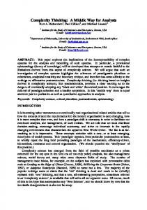

![[PDF] Psychology: Themes and Variations - Google Sites](https://m.moam.info/img/260x300/pdf-psychology-themes-and-variations-google-sites_6477e049097c4744708c3363.jpg)
![[PDF] Download Psychology: Themes Variations ... - Google Sites](https://m.moam.info/img/260x300/pdf-download-psychology-themes-variations-google-s_64771e5a097c474c228bac60.jpg)
