First European Conference on Earthquake Engineering and Seismology (a joint event of the 13th ECEE & 30th General Assembly of the ESC) Geneva, Switzerland, 3-8 September 2006 Paper Number: 1547
VARIATIONS OF APPARENT BUILDING FREQUENCIES - LESSONS FROM FULL-SCALE EARTHQUAKE OBSERVATIONS
Maria TODOROVSKA1, Mihailo TRIFUNAC2 and Tzong-Ying HAO3
SUMMARY A summary is presented of analyses of variations of the system frequency of 21 instrumented buildings in the Los Angeles area, which recorded the Northridge earthquake (MS= 6.7) of January 17, 1994, and some of its aftershocks. Some of these buildings also recorded other earthquakes, e.g. the 1971 San Fernando (ML = 6.6) and the 1987 Whittier Narrows (ML = 5.9) earthquakes and some its aftershocks. All the three earthquakes occurred within the metropolitan area and caused strong shaking and damage. The system frequencies were found to be the lowest during the strongest shaking from the main shock, suggesting system softening, and then increased during the aftershocks, suggesting system recovery. The observed temporary changes varied from one building to another, but did not exceed 30% for this data set. The system “recovery” was interpreted to be due to dynamic compaction of the soil during the (weak) aftershock shaking.
1.
INTRODUCTION
In most earthquake resistant design codes, the design shear forces are quantified using the seismic coefficient C(T), where T is the “fundamental vibration period of the building,” and various scaling factors that depend on the seismic zone, type of structure, soil site conditions, importance of the structure etc. As the building period cannot be measured for a particular structure before its construction, most codes provide simplified empirical formulae for its estimation, based on past experience and recorded response of existing buildings. The problem of estimation of T has been considered by many investigators, based on theory [Biot, 1942], small amplitude ambient and forced vibration tests of full-scale structures [Carder, 1936], and recorded earthquake response [Li and Mau, 1979]. The most reliable are the estimates of building periods obtained from recorded earthquake response. Such data are, however, extremely limited, both in quantity and in quality. The number of well-documented instrumented buildings that have recorded at least one strong earthquake is typically less than 100. When the recorded data is grouped by structural systems (moment resistant frame, shear wall etc.) and building materials (reinforced concrete, steal, etc.), the number of records per group becomes too small to control the accuracy of regression analyses, or to separate “good” from “bad” empirical models [Goel and Chopra, 1997; Stewart et al., 1999]. This problem is further complicated by the nonlinearity of the foundation soil even for very small strains [Hudson, 1970; Luco et al., 1987]. During strong earthquake shaking, the apparent period of the soil-foundation-structure system can lengthen significantly [Udwadia and Trifunac, 1974], and it may or may not return to its pre 1
Research Professor, University of Southern California, Civil Engineering Department, Los Angeles, CA 90089-2531, U.S.A. Email :
[email protected] 2 Professor, University of Southern California, Civil Engineering Department, Los Angeles, CA 90089-2531, U.S.A. Email:
[email protected] 3 Research Associate, University of Southern California, Civil Engineering Department, Los Angeles, CA 90089-2531, U.S.A. Email:
[email protected]
1
earthquake value. Environmental factors, such as temperature and heavy rainfall have also been found to cause small but systematic temporary changes [Clinton et al., 2006; Todorovska and Al Rjoub, 2006]. All of these factors contribute to the scatter in empirical regression analyses of building periods, and to ambiguity in choosing a representative T for evaluation of C(T) [Trifunac, 1999; 2000]. For further improvements and developments of the building codes, it is essential to understand the amplitude dependent period lengthening (as function of the level of response of the structure and strain in the soil), and estimate its range. This can be best accomplished by analysis of building periods from multiple earthquake recordings in buildings—of both small and large levels of shaking. The first step towards this goal is to augment the database of multiple earthquake records in buildings, which is very limited, because most buildings records have been recorded on film, and, mostly only those with larger amplitudes have been digitized and released. Data of small amplitude response is being generated fast from instrumented buildings with a digital recording system, but it may take many years before they record larger amplitude response. Hence, as far as the building design codes are considered, the use of small amplitude data from newly instrumented buildings is quite limited. While small amplitude data are useful in those buildings in which large amplitude response has already been recorded by analog recorders, replaced by the digital system, smaller amplitude analog recordings of past earthquakes are also very valuable—for understanding of the variations of building periods with time, which may be temporary or permanent. In the Los Angeles metropolitan area, there have been many small earthquakes and aftershocks of larger earthquakes that have been recorded in buildings and archived but not digitized and released. To this effect, an effort was initiated at the University of Southern California to augment the database of building periods estimated from multiple earthquake recordings, with the immediate objective to trace their variations with time and as a function of the level of response and understand their nature, and with the ultimate objective—to improve the code formulae for estimation of building periods. The effort consisted of digitization and processing of strong motion records in building in the Los Angeles area that have been archived at the U.S. Geological Survey (USGS), gathering of already processed data for the same buildings, and analysis of the building frequencies as a function of the level of response. This paper presents a summary of results for 21 buildings. Results for the first set of 7 buildings analyzed can be found in Todorovska et al. [2004a,b]. Similar analysis for a 7-story reinforced concrete hotel building in Van Nuys, damaged by the 1994 Northridge earthquake, can be found in Trifunac et al. [2001a,b], and for other instrumented buildings can be found in Hao et al. [2004], and Trifunac et al. (2001c,d,e).
2. METHODOLOGY The instantaneous frequency was estimated by two methods: (a) zero-crossing analysis, and (b) from the ridge of the Gabor transform, both applied to the relative roof displacement when there was a record at the base, or to the absolute displacement when only the roof response was recorded, and considered as an approximation of the relative displacement in the neighborhood of the first system frequency. Both methods were applied to the filtered displacement, such that it contained only motion in the neighborhood of the first system frequency, and resembled a chirp signal. The zero-crossing analysis consists of measuring the time between consecutive zero crossings of the displacement, and assuming this time interval to be a half of the system period (see Trifunac et al. [2001c,d,e]. The Gabor transform is a time-frequency distribution, which is up to a phase shift identical to a moving window analysis with a Gaussian time window. The instantaneous frequency was determined from the ridge of the transform, and the corresponding amplitude was estimated from the skeleton of the transform, which is the value of the transform along the ridge [Todorovska, 2001]. The results by both methods were found to be consistent, within the scatter.
3. DATA The data processed and analyzed was recorded in buildings in the Los Angeles metropolitan area that have been instrumented either by the USGS and partner organizations, or by the building owner (as required by the Los Angeles and state building codes), the latter being commonly referred to as “code” buildings. The data from these buildings have been archived by USGS, and are referred to in this paper as “USGS instrumented buildings,” identified by their station number. Figure 1 shows a map of the Los Angeles metropolitan area and locations of such buildings that were instrumented at the time of the 1994 Northridge earthquake.
2
The sensors in these buildings have been either three-component SMA-1 or multi-channel CR-1 accelerographs, both recording on film. Many of the “code” buildings (about 30 buildings total) have only one instrument, at the roof, due to a change in the original ordinance for Los Angeles, such that only one instrument at the roof was required, which lead to removal or neglect of the instruments at the ground floor and intermediate levels. This unfortunate fact limits considerably the use of these records, especially for analyses of soil-structure interaction. The recorded (absolute) roof motions can be used to estimate the apparent building period, as approximations of the relative roof motion near the first system frequency.
34.50 San Gabriel Mountains
San Fernando 1972
0
10
San Fernando Valley
34.25
km
5108
Sierra Madre, 1991 5453
5451 5455
5450
466
Pasadena, 1988
5259 5457 742 Los Angeles 5260 663 482 5456 793 572 872 5263 892 5082 530 5293 5277 5284 982 5233 Santa Monica 5460 5292 437 5459
Northridge and Aftershocks 1994
34.00
20
5258 229
Whittier Narrows and Aftershocks 1987 804
West Hollywood 2001
Malibu, 1989
5239
Montebello, 1989 5264
S. California 1989
Pacific Ocean
5106
33.75
5465 5462
San Pedro USGS instrumeneted building sites included in this analysis other USGS instrumeneted buildings
Long Beach 1933
Epicenters of earthquakes in the Los Angeles area
33.50
118.75
118.50
118.25
118.00
117.75
Figure 1 Locations of instrumented buildings in the Los Angeles metropolitan area at the time of the 1994 Northridge earthquake, for which the data is archived by USGS. The building sites are identified by their station number. After the Northridge earthquake, the analog strong motion instrumentation is being gradually replaced by digital, and additional buildings are being instrumented. For some of these buildings, data of smaller local earthquakes and distant larger earthquakes has been recorded and released. The recorded level of response for these events, however, is much smaller than that for the Northridge earthquake. Figure 1 also shows the epicenters of
3
earthquakes that have been recorded in these buildings. The Northridge main event was followed by a large number of aftershocks (9 of these had M > 5, and 55 had M > 4). Many of these larger magnitude aftershocks, as well as smaller magnitude but closer aftershocks, were recorded in the instrumented buildings. The aftershock of March 20, 1994 (M = 5.2; “aftershock 392”) was the one recorded by the largest number of (ground motion) stations [Todorovska et al., 1999]. The Northridge sequence was recorded on several films archived separately. The largest number of recorded aftershocks known to the authors of this paper is 86—at station USGS #5455, and about 60 at several other stations. Unfortunately, it turned out that the number of aftershock records useable for estimation of the building apparent frequency was small—up to 11. This paper shows results for 21 buildings for which there were three or more adequate records of both strong and weak shaking (mostly the 1994 Northridge sequence or the Whittier-Narrows sequence) to estimate the apparent building frequency. These stations are marked by open (yellow) dots in Fig. 1. The stations marked by solid rectangles, less than three “adequate” records for such analysis were known to exist, and were not included in this analysis.
Table 1. Earthquakes recorded by USGS instrumented buildings (1971 to 2001). Event San Fernando
Date
Time
ML
Latitude
Longitude
02/09/1971
06:00
6.6
34 24 42N
118 24 00W
Depth (km) --
Whittier-Narrows
10/01/1987
14:42
5.9
34 03 10N
118 04 34W
14.5
Whittier-Narrows, 12th Aft.
10/04/1987
10:59
5.3
34 04 01N
118 06 19W
13.0
Whittier-Narrows, 13th Aft.
02/03/1988
15:25
4.7
34 05 13N
118 02 52W
16.7
Pasadena
12/03/1988
11:38
4.9
34 08 56N
118 08 05W
13.3
Malibu
01/19/1989
06:53
5.0
33 55 07N
118 37 38W
11.8
Montebello
06/12/1989
16:57
4.4
34 01 39N
118 10 47W
15.6
Upland
02/28/1990
23:43
5.2
34 08 17N
117 42 10W
5.3
Sierra Madre
06/28/1991
14:43
5.8
34 15 45N
117 59 52W
12.0
Landers
06/28/1992
11:57
7.5
34 12 06N
116 26 06W
5.0
Big Bear
06/28/1992
15:05
6.5
34 12 06N
116 49 36W
5.0
Northridge
01/17/1994
12:30
6.7
34 12 48N
118 32 13W
18.4
Northridge, Aft. #1
01/17/1994
12:31
5.9
34 16 45N
118 28 25W
0.0
Northridge, Aft. #7
01/17/1994
12:39
4.9
34 15 39N
118 32 01W
14.8
Northridge, Aft. #9
01/17/1994
12:40
5.2
34 20 29N
118 36 05W
0.0
Northridge, Aft. #100
01/17/1994
17:56
4.6
34 13 39N
118 34 20W
19.2
Northridge, Aft. #129
01/17/1994
20:46
4.9
34 18 04N
118 33 55W
9.5
Northridge, Aft. #142
01/17/1994
23:33
5.6
34 19 34N
118 41 54W
9.8
Northridge, Aft. #151
01/18/1994
00:43
5.2
34 22 35N
118 41 53W
11.3
Northridge, Aft. #253
01/19/1994
21:09
5.1
34 22 43N
118 42 42W
14.4
Northridge, Aft. #254
01/19/1994
21:11
5.1
34 22 40N
118 37 10W
11.4
Northridge, Aft. #336
01/29/1994
11:20
5.1
34 18 21N
118 34 43W
1.1
Northridge, Aft. #392
03/20/1994
21:20
5.2
34 13 52N
118 28 30W
13.1
Hector Mine
10/16/1999
09:46
7.1
34 36 00N
116 16 12W
3.0
West Hollywood
09/09/2001
23:59
4.2
34 04 30N
118 22 44W
3.7
Table 1 shows a list of earthquakes recorded in “USGS” instrumented buildings. For the Northridge sequence, only the aftershocks are shown for which there is an adequate record that has been used in the analysis presented in this paper. For most of the buildings, the contributing aftershocks have not been identified. For this analysis, however, the amplitude of response and their chronological order were sufficient. This table also lists the 2001 West Hollywood earthquake (M = 4.2), which occurred close to many of the instrumented buildings (see Fig. 1), and which were likely recorded by these buildings.
4
4.
RESULTS
For each record considered for this analysis, the instantaneous system frequency was estimated and plotted versus time, and also versus the instantaneous amplitude of response. The latter curves were plotted on the same plot for all of the events, which made it possible to observe the variations of the system frequency as function of the amplitude of response during a particular earthquake, and also from one earthquake to another. Figure 2 shows such a plot for station USGS 5108 (Santa Susana ETEC Building No. 462), for data from the Northridge earthquake and its aftershocks, and for instantaneous frequency estimated by zero-crossing analysis. The horizontal axis shows the instantaneous frequency, and the vertical axis shows the amplitude of relative roof response expressed as a rocking angle in radians. The amplitudes of the response are those of the signal bandpas filtered near the first system frequency. The rocking angle was computed by dividing by the distance between the top and bottom instruments, estimated using average floor height of 12.5 feet (1 foot=30.48 cm) the amplitude of the relative (roof minus base) response, if motion at the base was recorded, or otherwise—the absolute horizontal response of the roof or top floor. It is noted here that this rocking angle includes the rigid body rocking, associated with soil-structure interaction, which could not be separated because of insufficient number of instruments at the base, in addition to motion resulting from deflection of the structure. USGS 5108: Canoga Park, Santa Susana -
ETEC Bldg #462
10 -3
θ max
Rocking angle (rad)
10 -4
EW Comp.
Aft. 129
NS Comp.
θ max
Zero-crossing method
Northridge (1994)
Zero-crossing method
10-3
Northridge (1994)
Aft. 253
10-4
Aft. 336
Aft. 129 Aft. 336 Aft. 142
Aft. 142 Aft. 151
10 -5 10 -5
Aft. 100
θ min
Aft. 7
Aft. 9
Aft. 9
10 -6 1.0
Aft. 392
Aft. 254
Aft. 392
θ min
Aft. 253
10 -6 1.5 fmin
2.0 fmax
2.5
Instantaneous system frequency -
1.0
1.5 fmin
fmax 2.0
Instantaneous system frequency -
Hz
2.5 Hz
Figure 2 Instantaneous frequency versus amplitude of motion for station USGS 5108.
Each point in Fig. 2 corresponds to a particular instant in time, and the points corresponding to consecutive instants of time are connected by a line. Different lines are used for different earthquake events. The first and last point for each event are marked respectively by an open and a closed circle. There is a considerable scatter in the estimates, mostly caused by violations of the assumption that the signals analyzed (the relative or absolute roof displacement) are asymptotic, which is the basic assumption for virtually all nonparametric methods for estimation of instantaneous frequency [Todorovska 2001; Todorovska and Trifunac 2006]. Asymptotic signals are such signals whose variation in time is mostly due to change in phase rather than change in amplitude. The asymptoticity assumption is violated most in the instants when the amplitudes of the signal are small and the amplitude modulation varies significantly. Despite the scatter in the data, the trend of the variation of system frequency with amplitude of response can be seen clearly in Fig. 2, and is marked by a backbone curve drawn approximately by hand. Such curves were drawn for all the stations. The common trend seen for most stations is a decrease of system frequency at the
5
Table 2. Maximum and minimum system frequencies and maximum and minimum rocking angles for 21 instrumented buildings. ∆f / f max
θ max
θ min
Hz
%
-3
×10 rad
-3
∆f / f max
θ max
θ min
Hz
%
-3
×10 rad
×10 rad
×10 rad
0.38
0.31
17.2
4.746
0.123
0.30
0.22
27.2
4.664
0.316
5
0.52
0.48
8.7
1.660
5
0.51
0.46
8.8
2.818
0.115
S72W
3
0.52
0.51
1.2
S18E
2
0.525
0.50
4.8
2.000
0.115
8
E00S
12
2.52
2.15
0.003
N00E
10
1.69
1.18
30.2
1.820
0.005
0793
11
S00W
5
0.98
2.754
0.008
E00S
6
0.92
0.72
21.7
2.344
0.010
0804
10
NS
2
15.0
0.500
0.017
EW
2
1.22
1.14
6.2
1.000
0.022
0872
8
N12W
0.57
9.5
1.698
0.042
S78W
3
0.76
0.63
17.1
1.995
0.021
0892
55
0.53
0.52
1.9
0.240
0.010
W83N
2
0.53
0.52
1.9
0.027
0.013
5082
2
1.16
1.01
12.9
1.820
0.013
S55W
2
1.19
0.94
21.0
1.622
0.016
NS
3
1.84
1.73
6.0
0.331
0.006
EW
3
1.85
1.76
4.9
0.260
0.010
6
E00S
9
2.13
1.65
22.6
0.496
0.003
N00E
7
1.90
1.52
19.7
1.056
0.004
5233
32
N62W
2
0.62
0.46
25.8
0.630
0.015
S28W
2
0.65
0.48
26.2
0.468
0.007
5239
7
N90E
5
0.90
0.81
10.0
0.741
0.005
S00W
5
0.81
0.76
6.2
1.622
0.008
5259
8
N00E
8
1.95
1.51
22.6
1.023
0.002
W00N
6
3.62
2.89
20.2
0.219
0.002
5260
12
W65N
7
0.83
0.71
14.5
0.300
0.016
S65W
9
0.80
0.68
15.0
4.169
0.020
5263
19
E70S
5
0.61
0.49
19.7
2.239
0.013
N70E
3
0.62
0.49
21.0
1.585
0.014
5450
9
N00E
5
0.69
0.61
11.2
3.088
0.039
W00N
5
0.67
0.58
13.5
5.166
0.038
5451
12
N00E
3
0.33
0.27
17.2
7.384
0.180
W00N
3
0.43
0.37
14.1
9.573
0.134
5453
9
N00E
4
0.61
0.43
29.2
7.870
0.061
W00N
8
0.74
0.71
5.7
4.881
0.026
5455
13
E30S
5
0.43
0.41
3.9
5.394
0.056
N30E
5
0.43
0.36
14.6
5.361
0.099
5457
10
N00E
8
0.68
0.57
15.8
6.340
0.029
S00W
7
0.87
0.70
18.6
3.625
0.013
No. rec.
f max
No. rec.
f max
Hz
Hz
N00E
3
W00N
3
12
NS
0.059
EW
0663
12
3.449
0.070
0742
14.7
0.400
0.79
19.4
0.80
0.68
3
0.63
N83E
2
6
N35W
5106
11
5108
No. floors
Comp.
0466
13
0482
Station No.
f min
6
Comp.
f min
-3
time of and shortly following the largest amplitudes of response to the main shock, and a recovery during the shaking by the aftershocks. The backbone curves were used to read roughly the range of the frequency changes and amplitudes of response, which are shown for the 21 buildings in Table 2. The percentage changes for all 21 buildings are plotted in Fig. 3. It is seen that, for the range of responses in this database, the change for most of the buildings does not exceed more than 25%, and it did not exceed 30% for any of the buildings included in this analysis. Results on further progress in this study will be posted at http://www.usc.edu/dept/civil_eng/Earthquake_eng/.
5.
SUMMARY AND CONCLUSIONS
This paper presents results on the changes of the apparent building frequency of 21 buildings in the Los Angeles area during multiple earthquake excitation, which caused both large and small amplitude response. Most of these buildings recorded the 1994 Northridge earthquake and some of its aftershocks. Although the number of recorded aftershocks in these buildings was large (up to about 80), only a small number of records were useable for this analysis, because of the small signal to noise ratio at short frequencies, especially for the tall buildings. The objective of the analysis was to estimate the trends and roughly the range of changes of the system frequencies during multiple earthquake shaking, both strong and weak. The system frequency was estimated by two methods—zero crossing and Gabor analysis. The results by both methods were found to be consistent. The general observed trend of the variation of the system frequency is decrease during the main event and recovery during the aftershocks. For most buildings, the frequency changed up to 25%, and it did not exceed 30% for this data set. The “recovery” is consistent with an interpretation that the change was mainly due to changes in the soil (rather than in the structure itself), or changes in the bond between the soil and the foundation. Other possible causes of the temporary changes are: contribution of the nonstructural elements to the total stiffness in resisting the seismic forces, and opening of existing cracks in the concrete structures during larger amplitude response. The degree to which each of these causes contributed to the temporary changes cannot be determined from the current instrumentation and is beyond the scope of this analysis.
35 742
30 466 5233
793 5263
5082
20
5457
5108
872 5260
5455
15
5450
5259
5451
∆f / f
max
%, Comp. 2
25
10
482 5239
5
804
5453
5106
663 892
0 0
5
10
15
20
25
30
∆ f / f max %, Comp. 1
Figure 3 Observed changes in system frequency for 21 buildings.
7
35
6.
ACKNOWLEDGEMENTS
This work was supported by U.S. Geological Survey External Research Program (Grants No. 03HQGR0013, and 20050176). All views presented are solely those of the authors and do not necessarily represent the official views of the U.S. Government. The authors are also grateful to Chris Stephens of the U.S. Geological Survey for kindly supplying film records for this project from the National Strong Motion Program archives.
REFERENCES Biot, M.A. (1942). Analytical and experimented methods in engineering seismology, Trans., ASCE, 68, 365409. Carder, D.S. (1936). Vibration observations, Chapter 5, in Earthquake Investigations in California 1934-1935, U.S. Dept. of Commerce, Coast and Geological Survey, Special Publication No. 201, Washington D.C. Clinton, J.F., Bradford, S,K,, Heaton, T.H., Favela, J. (2005). The observed wander of the natural frequencies in a structure, Bulletin of Seismological Society of America, 96(1):237-57. Goel, R.K., Chopra, A.K. (1997). Period formulas for concrete shear wall buildings, J. of Structural Eng., ASCE, 124(4), 426-433. Hao, T.Y., Trifunac, M.D., Todorovska, M.I. (2004). Instrumented buildings of University of Southern California—strong motion data, metadata and soil-structure system frequencies, Report CE 04-01, Dept. of Civil Engrg., Univ. of Southern California, Los Angeles, California, pp. 558. Hudson, D.E. (1970). Dynamic tests of full scale structures, Chapter 7, 127-149, in Earthquake Engineering, Edited by R.L. Wiegel, Prentice Hall, N.J. Li, Y., Mau, S.T. (1979). Learning from recorded earthquake motions in buildings, J. of Structural Engrg, ASCE, 123(1), 62-69. Luco, J.E., Trifunac, M.D., Wong, H.L. (1987). On the apparent change in dynamic behavior of a nine story reinforced concrete building, Bull. Seism. Soc. Amer., 77(6), 1961-1983. Stewart, J.P., Seed, R.B., and Fenves, G.L. (1999). Seismic soil-structure interaction in buildings II: Empirical findings, J. of Geotechnical and Geoenvironmental Engrg, ASCE, 125(1), 38-48. Todorovska, M.I. (2001). Estimation of instantaneous frequency of signals using the continuous wavelet transform, Report CE 01-07, Dept. of Civil Engrg., Univ. of Southern California, Los Angeles, California, pp. 55. Todorovska, M.I., Hao, T.-Y., Trifuna, M.D. (2004a). Building periods for use in earthquake resistant design codes - earthquake response data compilation and analysis of time and amplitude variations, Report CE 04-02, Dept. of Civil Engrg., Univ. of Southern California, Los Angeles, California, pp. 272. Todorovska, M.I., Hao, T.-Y., Trifunac, M.D. (2004b). Time and amplitude variations of building-soil system frequencies during strong earthquake shaking for selected buildings in the Los Angeles, Proc. Third UJNR Workshop on Soil-Structure Interaction, Menlo Park, California, March 29-30, 2004, pp. 22. Todorovska, M.I., Trifunac, M.D., Lee, V.W., Stephens, C.D., Fogleman, K.A, Davis, C., Tognazzini, R. (1999). The ML = 6.4 Northridge, California, Earthquake and Five M > 5 Aftershocks Between 17 January and 20 March 1994 - Summary of Processed Strong Motion Data, Report CE 99-01, Dept. of Civil Engrg., Univ. of Southern California, Los Angeles, California. Todorovska, M.I., Al Rjoub, Y. (2006). Effects of rainfall on soil-structure system frequency: examples based on poroelasticity and a comparison with full-scale measurements, Soil Dynamics and Earthquake Engrg, Biot Centennial Special Issue, in press.
8
Todorovska, M.I., Trifunac M.D. (2006). Damage detection in the Imperial County Services Building I: the data and time-frequency analysis, Soil Dynamics and Earthquake Engineering, submitted for publication. Trifunac, M.D. (1999). Comments on “Period formulas for concrete shear wall buildings,” J. Struct. Eng., ASCE, 125(7), 797-798. Trifunac, M.D. (2000). Comments on “Seismic soil-structure interaction in buildings I: analytical models, and II: empirical findings,” J. of Geotechnical and Geoenvironmental Engrg, ASCE, 126(7), 668-670. Trifunac, M.D., Ivanovic, S.S., Todorovska, M.I. (2001a). Apparent periods of a building I: Fourier analysis, J. of Struct. Engrg, ASCE, 127(5), 517-526). Trifunac, M.D., Ivanovic, S.S., Todorovska, M.I. (2001b). Apparent periods of a building II: time-frequency analysis, J. of Struct. Engrg, ASCE, 127(5), 527-537. Trifunac, M.D., Hao, T.Y., Todorovska M.I. (2001c). Response of a 14-story reinforced concrete structure to nine earthquakes: 61 years of observation in the Hollywood Storage Building. Report CE 01-02, Dept. of Civil Engrg., Univ. of Southern California, Los Angeles, California, pp. 88. Trifunac, M.D., Hao, T.Y., Todorovska, M.I. (2001d). On energy flow in earthquake response, Report CE 01-03, Dept. of Civil Engrg., Univ. of Southern California, Los Angeles, California. Trifunac, M.D., Hao, T.Y., Todorovska, M.I. (2001e). Energy of earthquake response as a design tool, Proc. 13th Mexican National Conf. on Earthquake Engineering, Guadalajara, Mexico. Udwadia, F.E., Trifunac, M.D. (1974). Time and amplitude dependent response of structures, Earthquake Engrg and Structural Dynamics, 2, 359-378.
9