c 2009 Institute for Scientific
Computing and Information
INTERNATIONAL JOURNAL OF NUMERICAL ANALYSIS AND MODELING Volume 1, Number 1, Pages 1–9
VECTOR-MATRIX MULTIPLICATION IN TERNARY OPTICAL COMPUTER YI JIN, XIAN-CHAO WANG, JUN-JIE PENG, MEI LI, ZHANG-YI SHEN, AND SHAN OU-YANG Abstract. This paper proposes a new means to complete the optical vectormatrix multiplication (OVMM). The OVMM is implemented on a novel optical computing architecture, ternary optical computer (TOC) by using modified signed-digit (MSD) number system. In addition, this study realizes optical addition in three steps, independent of the length of the operands, by four transformations in MSD, and discuses the multiplication of two MSD numbers in detail. A preliminary experimentation about the OVMM is performed on TOC. It illustrates the proposed method for OVMM is feasible and correct. Key Words. parallel, modified signed-digit, no-carry addition, basic operating unit, partial sum
1. Introduction Optical vector-matrix multiplication (OVMM) was proposed by Lee et al. in 1970[1]. Since then, many optical means have been put forward to implement OVMM[2-23]. However, most of them are analog computing systems only using light intensity, so their apparatus and experimental conditions are very sensitive to noise. In order to improve the accuracy, some algorithms and technologies were applied to OVMM, such as digital multiplication by analog convolution[7, 12], twos complement arithmetic[7, 11], error-correcting codes [6, 9], time-and-space integrating[12, 23], and digital partitioning[9]. In 2009, Li et al realized binary OVMM in ternary optical computer(TOC)[22]. But, Li’s work was short of application because every element in the matrix and vector was only one bit. On the other hand, numerical redundant representations have been used in nocarry addition or other arithmetic operations in the past several decades. It is most worth to mention that in those redundant representations, the modified signed-digit (MSD) number system is often used in optical computing[24, 25, 26]. The MSD, using three digits, -1, 0, and 1 with radix-2, has been proved to be well suited for realizing no-carry addition and other arithmetic operations. In the number system, the carry propagation occurs only between the neighboring positions in the addition operation and the results can be obtained through three logical steps by four logic operations. Therefore MSD is a parallel computing means. This paper will propose a method for OVMM via MSD number system in TOC. The remainder is organized as follows. Section 2 points the main technological foundations. Section 3 is the theory of the proposed method. Section 4 gives an experiment to verify the method. And the last section is a summary. 2000 Mathematics Subject Classification. 65Y05, 65Y10, 68Q10, 68W10. 1
2
Y. JIN, X. C. WANG, J. J. PENG, M. LI, Z. Y. SHEN, AND S. OUYANG
Figure 1. Architecture of the optical part in TOC. 2. Foundations 2.1. Optical Core of TOC Experimental System. The principle and architecture of TOC was proposed by Jin[28, 29]. In TOC, three steady states of light, no intensity light (NIL), horizontal polarization light (HPL) and vertical polarization light (VPL), are used to represent tri-valued information. In 2007 an experimental TOC system was built in Shanghai University. In the experimental system there is an optical core made of a light source, 5 pieces of vertical polarizer (VP1, VP2, VP3, VP4 and VP5), 2 pieces of horizontal polarizer (HP1 and HP2), 3 monochromatic liquid crystal arrays (L1, L2 and L3) and 1 photoreceptor array (D), shown in Figure 1. The core can be divided functionally into four components,a light source (S) , an encoder (E, including VP1, L1, VP2 and L2), a processor (O, containing VP3, HP1, L3, VP4, HP2, VP5 and L3), and a decoder (D). The optical processor (O) has four partitions from up to down, which are called respectively VV, VH, HV, and HH, shown in Figure 1. Each partition has the same structure: two pieces of polarizer holding a liquid crystal array, seeming like a sandwich. If there are a vertical polarizer and a horizontal polarizer in front and rear of L3, respectively, the partition is called VH, and so on. 2.2. Decrease-Radix Design Principle. In 2007, reference[30] proposed the 2 decrease-radix design principle (DRDP). The principle indicates: each of nn nvalued arithmetic unit without carry or borrow can be constructed by combining several simplest hardware units if there exists a special one (it is called D state in our work) included in the n physical states used to represent information. The sort of the simplest hardware units is n2 (n − 1), and they are called the basic operating-units(BOUs). Applying the DRDP to TOC, we can get the results as follows: • Any two-input tri-valued logic processor can be reconfigured by no more than 6 BOUs at any moment. And the total of the two-input tri-valued logic processors is 19683. • There are 18 kinds of the BOUs in total. • Each BOU is made of a liquid crystal pixel and a piece of polarizer on each side of it(see “O” in Figure 1). 2.3. MSD Addition. MSD was proposed by Avizienis in 1961[27], and was first used to optical computing by Draker in 1986. A number x can be represented in
VECTOR-MATRIX MULTIPLICATION IN TERNARY OPTICAL COMPUTER
MSD by the following equation: ∑ (1) x= xi 2i ,
3
xi ∈ {1, 0, 1},
i
where 1 denotes -1. In this paper, only MSD integer arithmetic operations are discussed. A number has several expression forms in MSD. For example, (4)10 = (100)2 or MSD = (1100)MSD = (11100)MSD , and (−4)10 = (1100)MSD = (11100)MSD . From the example, we can know that MSD is a number system with redundancy. The redundancy provides the possibility of no-carry addition in MSD. No-carry addition can be implemented by using four logical operations, called T, W, T0 , and W0 transformations, whose truth tables are shown in Table 1. The MSD addition can be explained by an example as follows. T 1 0 1 W 1 0 1 T´ 1 0 1 W´ 1 0 1 1 1 1 0 1 0 1 0 1 1 0 0 1 0 1 0 0 1 0 1 0 1 0 1 0 0 0 0 0 1 0 1 1 0 1 1 1 0 1 0 1 0 0 1 1 0 1 0 TABLE 1. Truth tables of four transformations used in MSD addition. Assume two MSD numbers x and y, x = 110110, y = 10010000. Step 1: Carry out logical operations T and W on x and y, and obtain their results, t and w, in parallel. By T, t = 10110110φ. By W, w = φ10100110. Where φ is a padded zero. Step 2: Carry out logical operations T0 and W0 on t and w, and obtain their results, t0 and w0 , in parallel. By T0 , t0 = 000100100φ. By W0 , w0 = φ111001010. Step 3: Carry out logical operation T on t0 and w0 , and obtain the final sum s of x and y. s = 0110000010. From the example, we can find that the no-carry addition can be implemented by four transformations in three logic steps which are independent of the length of operands. And the four kinds of logical operation units can be reconfigured by a large number of BOUs in TOC at any moment by DRDP. So the no-carry addition can be implemented by hardware in TOC. 2.4. MSD Multiplication. If a = an−1 a1 a0 and b = bn−1 b1 b0 , their product p is governed by the following equation: (2)
p = ab =
n−1 ∑ i=0
pi 2i =
n−1 ∑
abi 2i
i=0
It is clear that if bi is 0 the pi is also 0, if bi is 1 the pi is a, and if bi is 1 the pi is -a. So all pi (i = 0, . . . , n − 1) can be written out immediately from ai and bi in parallel by using a transformation. This transformation is also a tri-valued logic operation and marked with M. And then, the multiplication will be completed by adding up all abi 2i (i = 0, . . . , n − 1). Thus the multiplication will be implemented in parallel by hardware of TOC because all additions can be achieved by using the
4
Y. JIN, X. C. WANG, J. J. PENG, M. LI, Z. Y. SHEN, AND S. OUYANG
MSD additions in Section 2.3. An example is used to describe the operating process. M 1 0 1 1 1 0 1 0 0 0 0 1 1 0 1 TABLE 2. Truth tables of M transformation. Assume a = (14)10 = (1110)MSD , b = (9)10 = (1011)MSD then p = ab =
∑
pi 2i =
i
∑
abi 2i = (1110)MSD × (1011)MSD
i
= (1110)MSD × 1 + (1110)MSD × 1φ + (1110)MSD × 0φφ + (1110)MSD × 1φφφ = 1110 + 1110φ + 0φφ + 1110φφφ. Where the padded φs indicate (× 2i ). In other words, ∑ ∑ p = ab = pi 2i = abi 2i i
i
= (p0 × 2 + p1 × 2 ) + (p2 × 22 + p3 × 23 ) 0
1
= (1110 + 1110φ) + (0φφ + 1110φφφ). And then, the additions in two brackets can be completed via MSD means in parallel. After this, the last addition will be also completed by MSD addition. Because the TOC has a large number of data-bits, all sums ( pi 2i + pi+1 2i+1 ) can be completed in different regions of data-bits of optical processor in one machine instruction. 3. MSD Vector-Matrix Multiplication If α is a 1× N row vector and β is a N × N matrix , their product ψ is also a row vector and expressed as follows: (3)
N N N ∑ ∑ ∑ ψ = αβ = (ψ1 , ψ2 , . . . , ψN ) = ( αi βi1 , αi βi2 , . . . , αi βiN ). i=1
i=1
i=1
Obviously, from (3), all products αi βij (i, j = 1, . . . , N ) can be computed with the MSD multiplication and adding them up can be achieved with the MSD addition. Therefore the vector-matrix multiplication can be completed via a MSD means. The process of computing one of the vector-inner-products (VIPs) is shown in i Figure 2. In Figure 2, ψj,k is the jth partial sum of Step i in computing the VIP ψk (k = 1, . . . , N ). And q in Figure 2 is the maximum step-order in computing partial sums. It is easy to understand that q is equal to log2 N − 1 or the greatest integer which is less than log2 N . The broken-line boxes are padded 0 when the total of partial sums is odd in each step of computing the next-step partial sums. From the Figure 2, it can be seen that it is uncorrelated to compute all partial sums in each step. Therefore, all partial sums in the same step can be computed in parallel on a supercomputer or an optical computer. On the other hand, the TOC experimental system has three hundred data-bits and next-generation TOC system will have thousands of data-bits. Consequently, all partial sums in a computing step can be computed in parallel for normal task by utilizing these data-bits of TOC. So the vector-matrix multiplication can be completed in dlog2 N e steps if all the αi βij (i, j = 1, . . . , N ) are available.
VECTOR-MATRIX MULTIPLICATION IN TERNARY OPTICAL COMPUTER
5
Figure 2. The process of computing a VIP, that is, the element ψk of vector-matrix product. 4. Experiment and Results of the OVMM The technique of computing a vector-matrix multiplication by TOC can be described through an experiment as follows. In the experiment the vector α and matrix M are as follows: ( ) ) ( ) ( α = α1 α2 = 3 1 10 = 11 11 MSD , ( ) ( ) ( ) β11 β12 −1 2 11 10 β= = = , β21 β22 −2 −3 10 10 11 MSD and ψ = αβ =
(
11
11
)
( × MSD
11 10
10 11
) . MSD
The process of computing all the VIPs can be divided into two sequential parts. The former one computes all products of αi βij and the latter one computes all VIPs ψj (j = 1, 2) from the products. 4.1. Computing the Products of αi and βij in TOC. In the experiment there are four products of αi and βij , that is, α1 β11 , α2 β21 , α1 β12 , and α2 β22 . As αi and βij (i, j = 1, 2) are two bits, each product needs two 4-bit M. In other words, eight 4-bit M units are needed in total. Because the TOC has enough data-bits, the eight 4-bit M units will be structured in different areas of the optical processor in TOC(see Section 2.1). After all data being input, the eight 4-bit M units will be completed in one operation clock. Therefore, it is a parallel computing which is very different from electric computer. Following M transformation, MSD addition is activated to compute the products of αi and βij . For each βij being two bits, each product only needs one addition. Consequently, independent four additions will be needed. And each addition sequentially needs a 4-bit T and a 4-bit W, a 4-bit T0 and a 4-bit W0 , and a 4-bit T. In other words, computing all products successively needs four 4-bit T and four 4-bit W, four 4-bit T0 and four 4-bit W0 , and four 4-bit T. These additions can be achieved in different areas of the optical processor of TOC in parallel in three operation clocks. The concrete steps taken to compute these products are as follows. Step 1: In the O, construct eight 4-bit M units. Input the operands to corresponding M units. Run these M units on the optical processor. Get the output from the O. They are displayed in Figure 3(a). The results of the
6
Y. JIN, X. C. WANG, J. J. PENG, M. LI, Z. Y. SHEN, AND S. OUYANG
Figure 3. Output of optical processor in each step taken to compute the products of corresponding elements. To observe,real-line boxes mark the BOUs used by the first bit in each part, broken-line boxes mark the BOUs which light can pass through(LPBOU), and each BOU consists of 16 neighboring pixels. If the LPBOU is in VV or HV, the output is VPL which denotes 1; if the LPBOU is in VH or HH, the output is HPL which denotes 1 ; if there is no LPBOU, the output is NIL which denotes 0. M units are 0011, 0110, 0000, 0110, 0000, 0110, 0011, and 0110. Store the results into registers and recover data bits used by these M units. Step 2: In the O, construct four 4-bit T units and four 4-bit W units. Input the results of Step 1 to corresponding T and W units. Run these T and W units on the optical processor. Get the outputs from the O. They are displayed in Figure 3(b). The four group results of T are 0101,0110, 0110 and 0101, and those of W are 0101, 0110, 0110 and 0101. According to the MSD addition, each group results of T transformation need padding one zero as its least significant bit. We get 01010, 01100, 01100, and 01010 after padding zeros. And the new results are 1010, 1100, 1100, and 1010 after the frontal zero of each group being canceled. Store the results into registers and recover the data bits used by these T and W units. Step 3: In the O, construct four 4-bit T0 units and four 4-bit W0 units. Input the results of Step 2 to corresponding T0 and W0 units. Run these T0 and W0 units on the optical processor. Get the outputs from the O. They are displayed in Figure 3(c). The results of T0 are 0000, 0100, 0000 and 0000, and those of W0 are 1111, 1010, 1010 and 1111. Similarly, the results of T0 are altered into 0000, 1000, 0000, and 0000. Store the results into registers and recover data bits used by these T0 and W0 units. Step 4: In the O, construct four 4-bit T units. Input the results of Step 3 to corresponding T units. Run these T units on the optical processor. Get the
VECTOR-MATRIX MULTIPLICATION IN TERNARY OPTICAL COMPUTER
7
Figure 4. Outputs of optical processor in each step taken to compute VIPs from the products of corresponding elements. outputs from the O. They are displayed in Figure 3(d). The results of T are 1111, 0010, 1010 and 1111. Store the results into registers and recover the data bits used by these T units. Now, all products of αi and βij have been computed in four steps. They are, respectively, as follows: α1 β11 = (1111)MSD = (−3)10 , α1 β12 = (1010)MSD = (6)10 ,
α2 β21 = (0010)MSD = (−2)10 , α2 β22 = (1111)MSD = (−3)10 .
4.2. Computing the VIPs in TOC. According to Section 3, there are two VIPs, ψ1 and ψ2 , to be computed in the experiment. And ψ1 = α1 β11 + α2 β21 ,
ψ2 = α1 β12 + α2 β22 .
Therefore, independent two MSD additions will be conducted in the O. The steps are given as follows. Step 5: For each addition, construct a 4-bit T unit and a 4-bit W unit. Input the products of Step 4 to corresponding T and W units. Run these T and W units on the optical processor. Get the outputs from the O. They are shown in Figure 4(a). The results of T and W are 1101, 0101 and 1101, 0101, respectively. After being padded with zeros, the results are 11010, 01010 and 01101, 00101. Store the results into registers and recover the data bits used by these T and W units. Step 6: For each addition, construct a 5-bit T0 unit and a 5-bit W0 unit. Input the results of Step 5 to corresponding T0 and W0 units. Run these T0 and W0 units on the optical processor. Get the outputs from the O. They are shown in Figure 4(b). The results of T0 and W0 are 01000, 00000 and 10111, 01111, respectively. Store the results into registers and recover data bits used by these T0 and W0 units. Step 7: For each addition, construct a 5-bit T unit. Input the results of Step 6 to corresponding T units. Run these T units on the optical processor. The final outputs of O are displayed in Figure 4(c). From the last outputs of O, the results are 00111, 01111. That is ψ = αβ = (ψ1
ψ2 ) = (00111
01111)MSD = (−5
3)10 .
The experiment demonstrates the feasibility and correctness of the proposed OVMM on TOC. 5. Conclusions This paper has implemented a method for OVMM by five transformations in MSD number system on TOC experiment platform. The OVMM has two obvious advantages as follows:
8
Y. JIN, X. C. WANG, J. J. PENG, M. LI, Z. Y. SHEN, AND S. OUYANG
• It obtains the partial sums and VIPs in parallel. • It is easily expanded to thousands of bits. The operating speed isn’t discussed in detail because of the limitation of experimental condition. At the same time, the utilization of hardware is also not considered here. Acknowledgments The authors thank the support of the Shanghai Leading Academic Discipline Project (No.J50103), the National Natural Science Foundation of China (No.60473008), the Innovation Project of Shanghai University (No. A.10-0108-08-901) and the Research Project of Excellent Young Talents in the Universities in Shanghai (No. B.37-0108-08-002), and also thank the ternary optical computer lab for providing us with the optical platform. References [1] R. A. HEINZ, J. 0. ARTMAN, AND S. H. Lee, Matrix Multiplication by Optical Methods, APPLIED OPTICS, 9,1970,2161-2168. [2] J. W. GOODMAN, A. R. DIAS, AND L. M. WOODY, Fully parallel, high-speed incoherent optical method for performing discrete Fourier transforms,OPTICS LETTERS, 2,1978,1-3. [3] EUGENE P. MOSCA, RICHARD D. GRIFFIN, FRANK P, PURSEL, AND JOHN N. LEE, Acoustooptical matrix-vector product processor: implementation issues, Applied Optics, 28, 1989, 3843-3850. [4] R. P. BOCKER, Optical digital RUBIC (rapid unbiased bipolar incoherent calculator) cube processor. Opt. Eng., 23, 1984,26-32 [5] CAROLINE J. PERLEE, DAVID P. CASASENT, Effects of error sources on the parallelism of an optical matrix-vector processor. Applied Optics, 29, 1990,2544-2555. [6] SCOTT A. ELLETT, JOHN F. WALKUP, AND THOMAS F, KRILE, Error-correction coding for accuracy enhancement in optical matrix-vector multipliers, Applied Optics, 31, 1992, 5642-5653. [7] NAM Q. NGO, LE NGUYEN BINH, Fiber-optic array algebraic processing architectures, Applied Optics, 34, 1995,803-815. [8] W. T. RHODES, P. S. GUILFOYLE, Acousto-optic algebraic processing architectures, Proc. IEEE 72, 1984,820-830. [9] S. CARTWRIGHT, New optical matrix-vector multiplier. Applied Optics,23, 1984, 16831684. [10] D. CASASENT, S. RIEDL, Direct finite-element solution on an optical laboratory matrixvector processor, Opt. Commun., 65, 1988, 329-333. [11] A. P. GOUTOULIS, Systolic time-integrating acousto-optic binary processor, Applied Optics, 1984,23(22): 4095-4099. [12] E. J. BARANOSKI, D. P. CASASENT, High-accuracy optical processors: a new performance comparison, Applied Optics, 28, 1989, 5351-5357. [13] G. EICHMANN, Y. LI, P. P. HO, AND R. R. ALFANO, Digital optical isochronous array processing, Applied Optics,26, 1987, 2726-2733. [14] KHALED AL-GHONEIM, DAVID CASASENT, High-accuracy pipelined iterative-tree optical multiplication, Applied Optics, 33, 1994, 1517-1527. [15] P. LE, D. Y. ZANG, AND CHEN S. TSAI, Integrated electrooptic Bragg modulator modules for matrix-vector and matrix-matrix multiplications, Applied Optics, 27, 1988, 1780-1785. [16] NOBUO GOTO, YUKIHIRO KANAYAMA,AND YASUMITSU MIYAZAKI,Integrated optic matrix-vector multiplier using multifrequency acoustooptic Bragg diffraction, Applied Optics, 30, 1991, 523-530. [17] C. K. GARY, Matrix-vector multiplication using digital partitioning for more accurate optical computing, Applied Optics, 31, 1992, 6205-6211. [18] POCHI YEH, ARTHUR E. T. CHIOU, Optical matrix-vector multiplication through fourwave mixing in photorefractive media, Optics Letters, 12, 1987, 138-140. ¨ [19] MATTHIAS GRUBER, JURGEN JAHNS, STEFAN SINZINGER, Planar-integrated optical vector-matrix multiplier, Applied Optics, 39, 2000, 5367-5373.
VECTOR-MATRIX MULTIPLICATION IN TERNARY OPTICAL COMPUTER
9
[20] SHUQUN ZHANG, MOHAMMAD A. KARIM, Real-time digital optical matrix multiplication with a joint-transform correlator, Applied Optics, 38, 1999, 399-408. [21] SCOTT A. ELLETT, THOMAS F. KRILE, AND JOHN F. WALKUP, Throughput analysis of digital partitioning with error-correcting codes for optical matrix-vector processors, Applied Optics, 34, 1995, 6744-6751. [22] MEI LI, YI JIN, AND HUACAN HE, A New Method for Optical Vector-Matrix Multiplier, International Conference on Electronic Computer Technology (ICECT 2009),2009. [23] DAVID CASASENT, BRADLEY K. TAYLOR, Banded-matrix high-performance algorithm and architecture, Applied Optics, 24, 1985, 1476-1480. [24] B. L. DRAKER, R. P. BOCKER,AND M. E. Lasher etc, Photonic Computing Using the Modified Signed-Digit Number Representation,Optical Engineering,25, 1986, 038-043. [25] ABDALLAH K. CHERRI AND MOHAMMAD S. ALAM, Algorithms for optoelectronic implementation of modified signed-digit division, square-root, logarithmic, and exponential functions, APPLIED OPTICS, 40, 2001, 1236-1243 [26] GUOQING LI, FENG QIAN, HAO RUAN, AND LIREN LIN, Compact parallel optical modified-signed-digit arithmetic-logic array processor with electron-trapping device, APPLIED OPTICS, 38, 1999, 5039-5045 [27] A. AVIZIENIS, Signed-digit number representations for fast parallel arithmetic, IRE Trans. Electron. Comp., EC-10,1961,389-400. ¨ Ternary Optical Computer Principle,Science [28] YI JIN, HUACAN HE, AND YANGTIAN LU, in China (Series F), 46, 2003, 145-150. ¨ Ternary Optical Computer Architecture, [29] YI JIN, HUACAN HE, AND YANGTIAN LU, Physica Scripta, 2005,98-101. [30] JUNYONG YAN, YI JIN, AND KAIZHONG ZUO, Decrease-radix design principle for carrying/borrowing free multi-valued and application in ternary optical computer, Science in China(Series F), 51, 2008, 1415-1426. School of Computer Engineering and Science and High Performance Computing Center, Shanghai University, Shanghai 200072, China E-mail:
[email protected],
[email protected],
[email protected] School of Computer Engineering and Science, Shanghai University, Shanghai 200072, China School of Mathematics and Computational Science, Fuyang Normal College, Fuyang 236041, China E-mail:
[email protected] College of Computer Science & Engineering, Northwestern Polytechnical University, Xi’an 710072, China E-mail:
[email protected] School of Computer Engineering and Science, Shanghai University, Shanghai 200072, China Computer Science Department, Luoyang Normal University, LuoYang 471022, China E-mail: willian
[email protected]