GEOPHYSICS, VOL. 72, NO. 5 共SEPTEMBER-OCTOBER 2007兲; P. J65–J75, 11 FIGS., 1 TABLE. 10.1190/1.2766466
Vector-migration of standard copolarized 3D GPR data
Rita Streich1, Jan van der Kruk2, and Alan G. Green2
component algorithm, we derive an equivalent exact-field single-component vector-migration scheme that can be applied to most standard GPR data acquired using a single copolarized antenna pair. Our new formulation is valid for polarization-independent features 共e.g., most point scatterers, spheres, and planar objects兲, but not for polarization-dependent ones 共e.g., most underground public utilities兲. A variety of tests demonstrates the stability of the exact-field single-component operators. Applications of the new scheme to synthetic and field-recorded GPR data containing dipping planar reflections produce images that are virtually identical to the corresponding multicomponent vector-migrated images and are almost invariant to the relative orientations of antennas and reflectors. The new single-component vectormigration scheme is appropriate for migrating the majority of GPR data acquired by researchers and practitioners.
ABSTRACT The derivation of ground-penetrating radar 共GPR兲 images in which the amplitudes of reflections and diffractions are consistent with subsurface electromagnetic property contrasts requires migration algorithms that correctly account for the antenna radiation patterns and the vectorial character of electromagnetic wavefields. Most existing vector-migration techniques are based on far-field approximations of Green’s functions, which are inappropriate for the majority of GPR applications. We have recently developed a method for rapidly computing practically exact-field Green’s functions in a multicomponent vector migration scheme. A significant disadvantage of this scheme is the extra effort needed to record, process, and migrate at least two components of GPR data. By making straightforward modifications to the multi-
the space-frequency 共x-f兲 domain 共e.g., Moran et al., 2000; van Gestel and Stoffa, 2000; Wang and Oristaglio, 2000; van der Kruk et al., 2003a兲, whereas others depend on similar approximations formulated in the horizontal wavenumber-frequency 共k-f兲 domain 共Hansen and Johansen, 2000; Meincke, 2001, 2004兲. Most GPR targets are located at relatively short distances from the antennas 共e.g., for 100MHz antennas and a subsurface velocity of 0.1 m/ns, typical investigation depths may range from ⬃1 to ⬃15 m, corresponding to 1–15 wavelengths兲. Consequently, far-field approximations do not provide sufficient accuracy for many applications 共Annan, 1973; Radzevicius and Daniels, 2000a兲, and the resultant images may contain artifacts 共Streich et al., 2006; Streich and van der Kruk, 2007兲. To overcome these drawbacks, a fast and accurate method for computing practically exact-field radiation patterns was recently introduced by Streich and van der Kruk 共2007兲; their exact-field radiation patterns included the near-, intermediate-, and far-field contributions of infinitesimal dipoles located on a homogeneous halfspace 共Figure 1兲. Combining this new method with the imaging al-
INTRODUCTION The amplitudes and phases of raw ground-penetrating radar 共GPR兲 data depend on the antenna radiation patterns, the vector nature of electromagnetic wave propagation, and the electromagnetic properties of the subsurface 共e.g.,Annan, 2005兲. Our ultimate goal in migrating GPR data is to obtain images that accurately represent the subsurface electromagnetic property contrasts. Therefore, we need to eliminate the radiation-pattern and wave-propagation effects during the migration 共imaging兲 process. This requires vector-migration algorithms that explicitly account for the radiation patterns and vector-wave propagation; scalar algorithms developed primarily for migrating omnidirectional seismic data do not achieve this. A number of approximate vector-migration approaches have been developed to correct for radiation-pattern effects and vector-wave propagation. The majority of these are based on far-field approximations of Engheta et al. 共1982兲 to the radiation patterns expressed in
Manuscript received by the Editor October 10, 2006; revised manuscript received June 4, 2007; published online August 23, 2007. 1 Formerly ETH, Swiss Federal Institute of Technology, Institute of Geophysics, Zurich, Switzerland; presently SINTEF Petroleum Research, Trondheim, Norway. E-mail:
[email protected]. 2 ETH, Swiss Federal Institute of Technology, Institute of Geophysics, Zurich, Switzerland. E-mail:
[email protected];
[email protected]. © 2007 Society of Exploration Geophysicists. All rights reserved.
J65
J66
Streich et al.
gorithm described by van der Kruk et al. 共2003a兲 resulted in an accurate multicomponent vector-migration scheme that produced 3D images nearly devoid of radiation-pattern effects. There are numerous advantages in having multiple components of data. Independent information is contained in each component and combining components may improve signal-to-noise ratios. Moreover, multicomponent data are required for surveys aimed at deriving the properties of polarization-dependent scatter 共Radzevicius and Daniels, 2000b兲. Nevertheless, the effort to acquire, process, and migrate multicomponent data greatly exceeds that needed for conventional single-component data. It is desirable to have an accurate vector-imaging scheme that retains the advantages of the exact-
x1 E11
E22
E12
Air: ε r = 1
x2
Ground: ε r > 1
x3
Figure 1. Sketch showing the half-space model used for computing radiation patterns. E11 and E22 are copolarized antennas oriented in the x1- and x2-directions, respectively, and E12 are cross-polarized antennas. Input
Computations
Survey parameters, background velocity
~ 1) Evaluate k-f domain Green’s functions G (at oversampled wavenumbers) for initial depth x3ini (equations A-1–A-5) ~
2) Determine Green’s functions G at new depth x3 by vertical phase-shifting (equations A-6)
3) 2D IFFT to x-f domain
field multicomponent vector-migration scheme but is applicable to conventional single-component data. Since most existing GPR data sets comprise single-component records and single-component recording is likely to remain the standard in the foreseeable future, a single-component scheme would be of benefit to a wide range of GPR users. By reformulating algorithms described in van der Kruk et al. 共2003a兲 and Streich and van der Kruk 共2007兲, we have derived an exact-field single-component vector-migration scheme that provides accurate images of polarization-independent features 共e.g., most point scatterers, spheres, planar objects, etc.兲. Using only 50% of the data and roughly 60% of the computing resources, the new scheme produces images of dipping layers that are nearly identical to those supplied by the multicomponent approach. We begin by describing key aspects of the new single-component vector-migration scheme. We then demonstrate its ability to eliminate radiation-pattern effects and account for the vector character of the electromagnetic wavefield by demonstrating the equivalence of the multi- and single-component migration approaches. To do this, we use synthetic 3D GPR data generated for planar dipping reflectors, for which the recorded reflections only depend on the positions of the source and receiver antennas relative to the reflection points and on the corresponding radiation patterns. For zero-offset antennas, a planar dipping reflector has polarization-independent scattering coefficients; the incident electromagnetic wave is perpendicular to the reflector, such that the transverse-electric and transverse-magnetic reflection coefficients Output are equal. This is also approximately valid for small offsets between the antennas. For comparison, we also present standard scalar phase-shiftmigrated images and far-field multi- and singlecomponent vector-migrated images. Finally, we apply the new scheme to two copolarized 3D GPR data sets recorded across the same terrain using pairs of parallel antennas oriented approximately perpendicular to each other.
4) Shift matrix elements to obtain offset source ^ ^ and receiver Green’s functions G s and G r
THE SINGLE-COMPONENT VECTOR-MIGRATION ALGORITHM
5) x-f domain forward wavefield ^ (equations A-7–A-8) extrapolator D
6) 2-D FFT yields k-f domain ~ forward wavefield extrapolator D
~ 7) Inversion of D yields inverse ~ wavefield extrapolator F (equation A-9) ~ Recorded data E, transformed to k-f domain No
~ ~ 8) Multiply F with data E (equation A-10)
Single-frequency, single-depth ~ contribution to migrated image
9) All depth levels sampled? Yes ~ 10) For each depth level, sum over frequencies, 2D IFFT (equation A-11)
Migrated image
Figure 2. Flow chart showing the computation of multi- and single-component vectormigrated images. Bold letters are 2 ⫻ 2 matrices in multicomponent imaging and scalar quantities in single-component imaging. Symbols ˆ and ˜ indicate the x-f and k-f domains, respectively. For further details, see Appendix A.
Key elements of our vector-migration schemes are summarized in Figure 2 共van der Kruk et al., 2003a; Streich and van der Kruk, 2007兲. Although the flow diagram is primarily intended to show the exact-field formulations of our multiand single-component vector-migration schemes, steps 5–10 also describe the corresponding far-field schemes. Explicit formulations and equations for the multicomponent schemes are fully described in van der Kruk et al. 共2003a兲 and Streich and van der Kruk 共2007兲. The single-component vector-migration equations are derived in the same manner as the multicomponent ones. Formulations and equations for the single-component scheme are fully described in Appendix A. The vector-migration schemes comprise three primary procedures 共Figure 2兲:
Vector-migration of 3D GPR data
1兲
2兲 3兲
calculate vectorial Green’s functions that account for the source and receiver antenna radiation patterns and vector-wave propagation compute forward and inverse wavefield operators 共extrapolators兲 from the Green’s functions apply the inverse wavefield operator to the recorded GPR data to produce vector-migrated images
To facilitate the computation of the Green’s functions and achieve high computational efficiency, we combine k-f and x-f domain operations. At the beginning of the migration process, the decision is made to adopt either a multi- or single-component imaging approach. Previous applications of the vector-migration scheme outlined in Figure 2 were concerned only with the multicomponent options, yet conceptually a single-component approach can account for all of the vector information needed to produce a migrated image that accurately represents the subsurface physical properties 共see Appendix A兲.
Green’s functions: Antenna radiation patterns and vector-wavefield propagation To compute Green’s functions 共i.e., functions that describe the propagating electromagnetic field emitted by a point dipole source兲 that closely represent exact-field radiation-pattern and vector-wavepropagation effects for many surface-based GPR surveys 共steps 1–4 in Figure 2兲, we use a model in which horizontally oriented infinitesimal-dipole antennas are placed on a flat homogeneous ground 共Figure 1兲. For all of our vector-migration schemes, we require formulations of the source and receiver Green’s functions in the x-f domain. Computations of the Green’s functions are based on the survey parameters 共e.g., survey area, grid spacing, antenna offset兲 and an estimate of the background velocity. Far-field approximations of the Green’s functions are provided by explicit x-f domain formulas derived by Engheta et al. 共1982兲. These formulas can be efficiently and quickly evaluated 共note that in the analogous far-field vector-migration schemes direct evaluation of these formulas replaces steps 1–4 of Figure 2兲, but they may result in migration artifacts 共Streich et al., 2006; Streich and van der Kruk, 2007兲. In contrast, exact-field Green’s functions should provide artifact-free images, but computations of these functions are prohibitively expensive, because explicit expressions for them in the x-f domain are not available, and exact computations can only be carried out by numerical adaptive integration techniques 共Annan, 1973; Valle et al., 2001; Radzevicius et al., 2003兲. Fortunately, Streich and van der Kruk 共2007兲 have recently developed a rapid method for computing practically exact-field Green’s functions 共steps 1–3 in Figure 2兲. In applying Streich and van der Kruk’s 共2007兲 technique, we first evaluate explicit expressions for the exact-field Green’s functions in the k-f domain and then inverse fast Fourier transform 共2D IFFT兲 the
J67
output to obtain the corresponding x-f domain functions. To obtain accurate results from this procedure, it is necessary to account for the branch point singularities present in the k-f domain Green’s functions 共Annan, 1973兲. This is achieved by oversampling the k-f domain functions along the wavenumber axes. Oversampling in a horizontal direction is relative to the wavenumber sample interval determined by the length of the survey area in that direction 共equation A-5兲. Streich and van der Kruk 共2007兲 demonstrate that four to 16 times oversampling provides accurate estimates of exact-field x-f domain Green’s functions. For multicomponent migration, we use five different elements of the exact-field Green’s function tensor 共equation 1 of Streich and van der Kruk, 2007兲, whereas for single-component migration we only use the three elements relevant to a copolarized antenna configuration 共i.e., the expressions provided in either equation A-1 or A-2兲.
Forward/inverse wavefield operators and migration of the data Under the assumption that scattering is weak 共i.e., material contrasts are relatively small, such that the first-order Born approximation is applicable 关Born and Wolf, 1965兴兲, the x-f domain forward ˆ for both the multi- and singlewavefield operators 共extrapolators兲 D component schemes are equal to the inner products of the vectorial source and receiver Green’s functions 共step 5 in Figure 2兲. Spatial ˆ 共step 6兲 and inversion of the resulting Fourier transformation of D ˆ forward operator D at each point in the propagating wave regime of the k-f domain yields the inverse wavefield operator ˜F 共step 7兲. Multiplication of ˜F with the k-f domain representation of the recorded ˜ provides a single-frequency contribution to the k-f doGPR data E main-migrated image ˜ at depth x3 共step 8兲. Steps 2–8 are repeated for a sufficient density and number of depth levels to provide unaliased migrated images over the required depth range 共see step 9兲. It is not necessary to repeat the full evaluation of the k-f domain Green’s functions at each depth level. Rather, vertical-wavenumber phase shifting 共step 2; Slob et al. 2003兲 allows the k-f domain functions at all depth levels to be determined from those initially computed for depth x3. Finally, integration over frequency for each depth level followed by spatial IFFT yields the space-domain migrated image 共step 10兲. ˜ , and ˜F, the data ˆ,D In multicomponent migration, the operators D ˜ E, and the image are 2 ⫻ 2 matrices and the computations in steps 5–8 共Figure 2兲 are matrix operations 共Streich and van der Kruk, 2007兲. The multicomponent imaging operator is obtained by inverting a 2 ⫻ 2 matrix that contains the co- and cross-polarized forward operator elements 共see step 6 of Figure 5 in Streich and van der Kruk, 2007兲. In single-component migration, the operators, data, and image are scalars and the computations are scalar operations. 共The single-component imaging operator is obtained by inverting a single copolarized forward operator; see equation A-9兲. For example, the at depth x3 in the element ˜MC 11 of the multicomponent image matrix ˜
J68
Streich et al.
Some properties of the inverse wavefield operators ˜F
k-f domain is given by
Figure 3 shows a comparison between the two multicomponent ˜ MC imaging operator elements ˜FMC 11 and F 12 and the single-component = + 共1兲 SC ˜ operator F11 computed for the same model. Since the single-component imaging operator ˜FSC 11 is based on the inverted forward wavewhereas the equivalent single-component image ˜SC 11 is given by field operator in the wavenumber domain, it has high amplitudes at 共equation A-10兲 wavenumbers for which low amplitudes are measured, such as about the k1-axis and at angles around ±45° to the k1 and k2 axes 共Figure 3c兲. Similarly, it has low amplitudes at wavenumbers for which high SC SC˜ ˜ ˜11 = F11 E11 . 共2兲 amplitudes are measured, such as about the k2-axis. For the multicomponent imaging operators, ˜FMC 11 amplifies data present about the In equations 1 and 2, subscripts 1 and 2 are associated with the x1 and mainly amplifies data present at angles around k1-axis, whereas ˜FMC 12 x2 antenna orientations and electric-field directions 共i.e., ˜E11 signifies ±45° to the k1-and k2-axes. Single- and multicomponent migration of copolarized antennas oriented in the x1-direction and ˜E21 signifies synthetic point-scatterer data yield practically identical images. In cross-polarized antennas兲 and superscripts MC and SC refer to the both cases, the images have unit amplitudes in the k-f domain after multi- and single-component operators and images. We emphasize multiplying the respective imaging operators with the data 共see van ˆ ˜ mc that ˜Fsc der Kruk et al., 2003a兲, even though the single- and multicomponent 11 ⫽ F 11 , that the single-component scalar operator D includes the vectorial radiation-pattern and wave-propagation effects for the images are obtained from different data components 共copolarized copolarized source-receiver pair, and that application of the scalar versus co- and cross-polarized兲 and different imaging operators imaging operator ˜F removes these effects from single-component 共scalar versus 2 ⫻ 2 matrix兲. GPR data. Previously, van der Kruk et al. 共2003a兲 had asserted that far-field single-component imaging operators would have unbounded amplitudes in a homogeneous half-space. By comparison, our extensive ~ MC ~MC ~SC a) b) c) numerical experiments demonstrate that the properties of the exactF 12 F 11 F 11 field single-component imaging operators in a homogeneous half–5 –5 –5 space are similar to those of the exact-field multicomponent ones; 0 0 0 both have bounded amplitudes. A critical issue is the behavior of the 5 5 5 operators close to the surface. To compensate for the high energy present near a source antenna, stable inverse imaging operators –5 0 5 –5 0 5 –5 0 5 should have low amplitudes as the depth x3 approaches 0 m. k1 (m–1) k1 (m–1) k1 (m–1) In Figure 4, we show the maximum amplitudes of the multi- and –3 –3 –3 2 4 x10 1 2 x10 2 4 x10 single-component imaging operators at progressively shallower depths for the permittivities and center frequencies of our synthetic Figure 3. Examples of multi- and single-component imaging operaand field data sets. Information for operators based on both the fartors computed from exact-field Green’s functions for r = 5.32 共i.e., and exact-field Green’s functions are presented. The increasing valthe value used for imaging our field data兲, f = 80 MHz and x3 MC ˜ ues of the three far-field operators with decreasing depth in Figure 4a = 10 m. 共a兲 Copolarized element F11 of multicomponent operator, and the strongly increasing values in Figure 4b, which are caused by of multicomponent operator, and 共b兲 cross-polarized element ˜FMC 12 sharp minima in the far-field Green’s functions 共Engheta et al., 共c兲 single-component operator ˜FSC 11 共subscripts for this scalar quantity identify the orientation of the copolarized antennas in the 1982兲, are evidence that significant instability can occur for some x1-direction兲. The white circles mark the outer limit of the propagatcombinations of model and frequency. In contrast, the amplitudes of ing wave region in the subsurface. For the same colors, the ampliall exact-field operators remain similarly small over the entire distudes in 共b兲 are one-half those of 共a兲 and 共c兲. played shallow depth range, demonstrating that the single-component operators are as stable as a) b) f = 70 MHz, εr = 7 f = 80 MHz, εr = 5.32 the multicomponent ones. Because we have ne104 100 ~ far,MC ~ exa,MC glected parts of the evanescent field in the forF 11 F 11 ~ far,MC ~ exa,MC ward computation of the exact-field Green’s F F 12 12 102 10–1 ~ far,SC ~ exa,SC functions, the amplitudes of the inverse imaging F 11 F 11 operators do not decrease with decreasing depth, 100 10–2 as they should. Consequently, our exact-field operators for depths shallower than 1/10 to 1/3 of a 10–3 10–2 wavelength are inaccurate 共Streich and van der Kruk, 2007兲. Maximum amplitude of F
k2 (m–1)
˜FMC˜E , 12 21
k2 (m–1)
˜FMC˜E 11 11
Maximum amplitude of F
k2 (m–1)
MC ˜11
10–4 100
10–1
10–2 10–3 x3 (m)
10–4
10–5
10–4 100
10–1
10–2 10–3 x3 (m)
10–4
10–5
Figure 4. Maximum amplitudes of multi- and single-component imaging operators computed from far- and exact-field Green’s functions as depth x3 approaches zero. Offset between antennas is 1 m. Example in 共a兲 with r = 7 and f = 70 MHz is relevant to our synthetic data and example in 共b兲 with r = 5.32 and f = 80 MHz is relevant to our field data. Superscripts far and exa indicate far-field and exact-field operators and superscripts MC and SC indicate multi- and single-component operators.
APPLICATION TO SYNTHETIC DATA Models and computational details A 3D finite-difference time-domain algorithm 共Lampe et al., 2003兲 was used to generate syn-
Vector-migration of 3D GPR data
For the standard scalar phase-shift images, the average peak-topeak reflection amplitude in the model 1 gzd 11 image is 41% higher than that in the gzd 22 image 共Figures 6a–c, 8a and b兲, slightly higher than the 39% amplitude difference of the nonmigrated images. Note the 90° phase shift in these images relative to the others 共best seen in Figure 8; van der Kruk et al., 2003b兲. To analyze the image amplitudes without this phase shift, we recomputed the scalar phase-shift migrated images using a modified algorithm that included a 90° phase correction and a geometric spreading correction 共van der Kruk mgzd traces in Figure 8兲. This resulted in an averet al., 2003b兲; see ␣␣ age amplitude difference of 42%. Although the far-field multi- and single-component images are practically identical for each antenna orientation 共compare the blue solid and red dashed lines in Figure 8a and b兲, the average peak-toand far,SC images differ peak reflection amplitudes of the far,MC 11 11 far,MC far,SC from those of the 22 and 22 images by 30% 共Figures 6d–i, 8a and b兲. Clearly, the phase-shift and far-field images are unsatisfactorily dependent on the antenna orientations. In contrast, the peak-to-peak reflection amplitudes of all exactfield multi- and single-component images for model 1 are very close to each other 共Figures 6j–o, 8a and b兲, with average differences of about 2.6%. These small residual differences are likely caused by forward modeling artifacts and slight reflection coefficient variations for the different antenna orientations 共rotating the 1-m offsetbroadside antennas 90° around a fixed midpoint yields maximum amplitude variations of ⬍1% because of changes in the reflection coefficients that result from the small antenna offset兲.
a) x2
b) x2
R1
R1 T1
T1
T2 T2
χ11
° 18
thetic 3D common-offset data from a model that contained an 18° dipping boundary with relative permittivities r = 7 above and r = 10 below and a constant conductivity = 0.2 mS/m. The dimensions of the 3D model were 7.4⫻ 6.8⫻ 5 m. Sources emitting a wavelet represented by the derivative of a Gaussian function with a center frequency of 70 MHz were simulated on a 0.1⫻ 0.1 m surface grid. The source-receiver offset was 1 m. Copolarized data were generated for dipole antennas oriented at 0°, 90°, and 45° 共models 1 and 2; Figure 5兲 relative to the trend of the reflector. Corresponding cross-polarized data were also generated. Because the angles of incidence are small for the small antenna offsets, the amplitudes of reflections from these planes should be practically independent of the polarization of the incident wavefield. Accordingly, eliminating the radiation patterns and vector-wavefield effects via accurate vector-migration should result in practically equal image amplitudes and phases for the antennas differently oriented. This is best tested by comparing the 11 and 22 images obtained for model 1 because the amplitude differences are a maximum between the raw data acquired with these particular orthogonal antenna orientations; for the central survey area of this model, the average peak-to-peak reflection amplitude of the nonmigrated data simulated for the 0°-oriented antennas is 39% higher than that simulated for the 90°-oriented antennas. Correct vector-migration should also yield equal amplitudes in the corresponding multi- and single-component images. We test this aspect by comparing the multi- and single-component images of the reflector in model 2. The amplitudes of the cross-polarized data are a maximum for this geometry 共Lehmann et al., 2000兲, contributing significantly to the multicomponent images. After muting the direct waves, which are not accounted for in our imaging schemes, we migrated the synthetic 3D GPR data using a scalar phase-shift algorithm 共Gazdag, 1978兲 and the far-field multicomponent 共van der Kruk et al., 2003a兲, far-field single-component, exact-field multicomponent 共Streich and van der Kruk, 2007兲, and exact-field single-component vector-migration schemes. From each algorithm, we obtained the 11 and 22 images for model 1 and the 11 image for model 2 共Figure 5兲. In applying the exact-field algorithms, 16 times oversampling was used for computing the x-f domain Green’s functions. Along selected transects, we have compared the practically exact-field x-f domain Green’s function values with highly accurate values obtained using computationally expensive adaptive integration 共Streich and van der Kruk, 2007兲. These tests indicated errors in the practically exact-field Green’s functions of ⬍1% throughout the 5-m depth range of interest. The times required to compute single complete migrated images on a 3.2 GHz CPU are summarized in Table 1. For all computations, we used 45 frequency components in a 25–207 MHz range and 110 depth levels at 0.05-m intervals down to 5.5 m.
J69
R2
T1 T2
χ22
χ11
18° x1
x1
Figure 5. Geometry of synthetic surveys for a reflector trending 共a兲 parallel and 共b兲 at 45° to the x1-axis: Within each set of antennas 共underlain in gray兲, T␣ and R are the transmitting and receiving antennas used to obtain the E␣ components; 11 and 22 represent the multi- and single-component images associated with the respective antenna sets. Lines with ticks show the trends and dips of the model reflectors and dashed lines indicate typical wave-propagation paths.
Table 1. Computation times for the various migrations of the synthetic data.
Migrated images
Migration algorithm
Vertical slices extracted from the various migrated images 共Figures 6 and 7兲 and selected traces 共Figure 8兲 highlight the reflection from the dipping layer boundary. We have not deconvolved the source wavelet from the data. As a result, the layer boundary 共dashed lines in Figures 6 and 7兲 coincides with the emergent onsets of the reflection.
Scalar phase-shift Far-field multicomponent Far-field single-component Exact-field multicomponent Exact-field single-component
Time 共hours兲 0.24 0.45 0.28 15.0 8.4
J70
Streich et al.
For model 2, the amplitudes of the far-field multi- and single-component vector-migrated images differ by 13% 共Figure 7b and c; compare the blue solid and red dashed lines in Figure 8c兲. This is likely caused by errors in the far-field approximation propagating differently into the multi- and single-component images. By comparison, the exact-field multi- and single-component images for model 2 are practically identical to each other 共Figures 7d and e and 8c兲 and to theequivalent images produced for model 1 共Figures 6j, k, m, and n; 8a and b兲. Taken together, these results confirm that the exact-field multiand single-component vector-migration schemes equivalently correct for the radiation patterns, and that for polarization-independent scatterers only one copolarized antenna pair is required for accurately imaging the subsurface. As for all migration schemes, the quality of the final images is dependent on the accuracy of the velocity model 共Yilmaz, 2001兲. We have investigated the effects of using velocities erroneous by up to
±10% on the imaging of the model 1 data. Incorrect velocities result in errors in the radiation patterns and the amplitude distributions of the imaging operators 共e.g., the maxima about the k1-axis and minima about the k2-axis in Figure 3a and c would appear at lower wavenumbers for erroneously low velocities and at higher wavenumbers for erroneously high velocities兲. Consequently, velocity errors not only result in reflector mislocations, but also in larger differences between the exact-field 11 and 22 images. As examples, background velocities 2% and 10% too high caused differences between exa,SC 11 and exa,SC of 1.7% and –2.5%, and velocities 2% and 10% too low 22 caused differences of 3.7% and 8.1%, respectively 共compare these values to the 2.6% error obtained using the correct velocity兲.
APPLICATION TO FIELD DATA
Depth (m)
Depth (m)
Relative amplitude
Depth (m)
Depth (m)
Depth (m)
We have tested the exact-field single-component vector-migration scheme on GPR data acquired at a gravel pit in northern Switzerland. In the process of quarrying at this site, an artificial bank of well-sorted gravel was deposited gzd gzd gzd gzd temporarily on a dipping surface of less homogea) b) c) χ 11 χ 22 χ 11 – χ 22 neous natural gravel deposits 共Figure 9a兲. Prelim2 2 2 inary tests demonstrated that the interface be3 3 3 tween these two gravel units, which dipped at approximately 35° 共near the angle of repose兲 and 4 4 4 was nearly planar, produced a strong GPR reflec1 2 3 4 m 1 2 3 4 m 1 2 3 4 m far,MC far,MC far,MC d) e) f) χ 11 χ 22 χ far,MC – χ 22 tion. 11 We collected 3D GPR data in a 40⫻ 9 m area 2 2 2 that extended across the surface of the artificial 3 3 3 bank and adjacent natural deposits. Two single4 4 4 component data sets were recorded using copolarized antennas offset by 1 m. The antennas 1 2 3 4 m 1 2 3 4 m 1 2 3 4 m far,SC far,SC far,SC χ 11 χ 22 χ far,SC h) g) i) – χ 22 11 were oriented approximately perpendicular to the 1 reflector trend for the E11 data and approximately 2 2 2 parallel for the E22 data 共Figure 9b兲. For each data 0 3 3 3 volume, the inline and crossline trace spacings 4 4 4 were mostly 0.1–0.15 m and about 0.25 m, re–1 1 2 3 4 m 1 2 3 4 m 1 2 3 4 m spectively. exa,MC exa,MC exa,MC j) k) l) χ 11 χ 22 χ exa,MC – χ 22 11 Because our single-component vector-migration scheme requires the antennas to be oriented 2 2 2 exactly parallel to one of the coordinate axes, we 3 3 3 processed and migrated the two data sets in 4 4 4 slightly different coordinate systems. The data 1 2 3 4 m 1 2 3 4 m 1 2 3 4 m were interpolated onto uniform 0.125⫻ 0.125 m exa,SC exa,SC exa,SC m) n) o) χ 11 χ 22 χ exa,SC – χ 22 11 grids using Delaunay triangulation. We account2 2 2 ed for the effects of surface topography by fitting a reference plane through the slightly undulating 3 3 3 surface and then applying a static shift to each 4 4 4 trace that compensated for the distance of the ac1 2 3 4 5 1 2 3 4 5 1 2 3 4 5 tual surface from this plane 共Streich et al., 2006兲. x2 (m) x2 (m) x2 (m) Application of a common gain function 共the inverse of the average trace envelope兲 reduced the Figure 6. For synthetic data obtained from model 1 共Figure 5a兲, x2-directed cross sections direct wave energy while preserving relative amextracted from 共a and b兲 scalar phase-shift, 共d and e兲 far-field multicomponent, 共g and h兲 far-field single-component, 共j and k兲 exact-field multicomponent, and 共m and n兲 exactplitude information within and between the two field single-component 3D migrated images. Subscripts 11 and 22 correspond to copolardata volumes. A velocity of 0.13 m/ns 共i.e., r ized antennas oriented in the x1- and x2- directions 共Figure 1兲. The angle between the re⬃5.3兲 determined from common-midpoint data flector trend and the copolarized antennas is 0° for 11 and 90° for 22 共see Figure 5a兲. recorded parallel to the trend of the reflecting inDashed lines show the reflector position. Arrows indicate the locations of traces shown in Figure 8a and b. The right column shows the respective differences 11 − 22. terface was used for migrating the data.
Vector-migration of 3D GPR data
as for the far-field vector-images, the average amplitude ratio is 1.35 and the standard deviation is 0.46 共Figure 11c and d兲. In marked contrast, for the exact-field vector-migrated images, the amplitude ratio is reduced to 1.09, which is close to the ideal value of 1, and the standard deviation is only 0.30 共Figure 11e and f兲. These results indicatethat exact-field single-component vector-migration has eliminated most radiation-pattern and vector-wave-propagation effects from the field data. The residual amplitude differences may be caused byvarious factors, including 共1兲 variable antenna-ground coupling, 共2兲 discrepancies between the employed dipole antenna model and real GPR antennas, 共3兲 spatial variations in GPR velocity, 共4兲 temporal velocity variations resulting from rainfall during the collection of the E11 data, and 共5兲 non-Born scattering effects.
gzd χ 11
2 3 4 1
Depth (m)
4
m
4
m
2 3 4 1
2
3
far,SC χ 11
c) Depth (m)
3
far,MC χ 11
b)
1
2 3
0
4 1
2
3
4
m
4
m
4
5
–1
exa,MC χ 11
d) Depth (m)
2
Relative amplitude
Depth (m)
a)
2 3 4 1
2
3
exa,SC χ 11
e) Depth (m)
The processed data were imaged using the modified scalar phaseshift scheme and the far and exact-field single-component vectormigration schemes. We computed the exact-field Green’s functions using fourfold oversampling, which resulted in wavenumber sample intervals similar to those used for imaging the synthetic data. The computations for 47 frequency components in the range of 40–123 MHz and 500 depth levels down to 25 m at 0.05-m intervals required 5.7 hours for the far-field and 45.5 hours for the exact-field vector-migrations. For amplitude analysis and display purposes, all imaged data volumes were rotated to a common coordinate system in which the x1-axis was parallel to the reflector dip direction 共Figure 9b兲. Vertical sections of the images are displayed in Figure 10. The reflection from the interface between the artificial bank and the naturally deposited gravels 共marked by arrows in Figure 10兲 is the most prominent event in all images. Weaker parallel reflections above this interface originate from minor layer boundaries within the artificial bank deposits. Below the principal interface reflection, a number of near-parallel dipping events appear only in images produced from the E11 data. Their moveouts and traveltimes indicate that they are reflections from trees located northwest of the survey area 共not seen in Figure 9a, but sketched in Figure 9b兲. The geometry of the electric field generated by the E11 antenna configuration is nearly ideal for inducing reflections from the tree trunks, whereas that for the E22 configuration is nearly ideal for suppressing such reflections 共van der Kruk and Slob, 2004兲. Furthermore, the apparent dips of the tree reflections coincide with high-amplitude regions in the vector-imaging operators for the E11 data and low-amplitude regions in the operators for the E22 data, such that imaging enhances these reflections in the 11 images 共Figure 10c and e兲 and reduces them in the 22 images 共Figure 10d and f兲. The amplitudes of all subsurface reflections differ significantly between the modified scalar phase-shift images 11mgzd and 22mgzd and far between the far-field vector-images far 11 and 22 , but they are similar exa exa in the exact-field vector-images 11 and 22 . To assess quantitatively the performance of the different migration schemes, we have compared the amplitudes of the principal interface reflection observed in the various 11 and 22 images. We picked peak-to-peak amplitudes using the strongest negative troughs 共colored brown and marked by arrows in Figure 10兲 and the positive peaks below. The amplitudes determined from the 11 and 22 images are compared for each of the migration schemes in Figure 11b, d, and f, and the distributions of amplitude ratios 22 /11 are shown superimposed on the picked reflection surface in Figure 11a, c, and e. For each pair of migrated images, we only show picked reflection amplitudes that are well above background values in both images. For the modified scalar phase-shift migrated images, the amplitude analysis yields an average 22 /11 amplitude ratio of 1.77 with a relatively high standard deviation of 0.74 共Figure 11a and b兲, where-
J71
2 3 4 1
2 3 x2 (m)
Figure 7. For synthetic data obtained from model 2 共Figure 5b兲, x2-directed cross sections extracted from the 共a兲 scalar phase-shift, 共b兲 far-field multicomponent, 共c兲 far-field single-component, 共d兲 exact-field multicomponent, and 共e兲 exact-field single-component 3D migrated images. Subscripts 11 correspond to copolarized antennas oriented in the x1-direction 共Figure 1兲. The angle between the reflector trend and the copolarized antennas is 45° 共see Figure 5b兲. Dashed lines show the reflector position. Arrows indicate the locations of traces shown in Figure 8c.
J72
Streich et al.
Amplitude
a)
b)
0°
c)
90°
45°
1
1
1
0
0
0
–1 2.5
3
χ gzd αα
χ mgzd αα
χ far,MC αα
χ far,SC αα
χ exa,MC αα
χ exa,SC αα
3.5
4
–1 2.5
z (m)
3
3.5
4
2.5
3
z (m)
3.5
4
z (m)
Figure 8. Traces extracted from the various images of a synthetic dipping planar reflector. Traces from the scalar phase-shift images gzd ␣␣ , modifar,MC fied scalar phase-shift images mgzd and far,SC ␣␣ , far-field multi- and single-component images ␣␣ ␣␣ , and exact-field multi- and single-component images exa,MC and exa,SC are shown. Subscripts ␣␣ represent 11 or 22, corresponding to copolarized antennas oriented in the x1- or x2-directions ␣␣ ␣␣ 共Figure 1兲. For all images, the copolarized antennas are oriented at 共a兲 0°, 共b兲 90°, and 共c兲 45° relative to the reflector trend 共see model geometry in Figure 5兲.
mgzd χ 11
a)
a)
5 x3 (m)
5 x3 (m)
mgzd χ 22
b)
10 15
10 15
Survey area ~40 x 9 m
Natural deposits
Bank of well-sorted gravel
30
25
20 15 x1 (m)
10
far χ 11
c)
30
Trees
E11
10
5 x3 (m)
x3 (m)
N
x2 Reflector
20 15 x1 (m) far χ 22
d)
5
b)
25
10 15
10 15
E22 x1
area Survey
30
25
Reflector
10
exa χ 11
e)
30
25
20 15 x1 (m)
10
exa χ 22
f)
5
5 x3 (m)
x3 (m)
Figure 9. 共a兲 Photograph showing the Weiach survey site. The measurements were made on the planar surface of an artificial gravel bank. The white arrow identifies the boundary between this gravel unit and the underlying natural gravel deposits. 共b兲 Top-view showing the relative orientations of the antennas, survey area 共dashed box兲, coordinate system adopted for displaying the results and trees near the northwest edge of the survey area.
20 15 x1 (m)
10 15
10 15
30
25
20 15 x1 (m)
10
30
25
20 15 x1 (m)
10
Figure 10. Vertical slices extracted at x2 = 11.25 m from the 共a and b兲 modified scalar phase-shift, 共c and d兲 far-field single-component vector and 共e and f兲 exact-field single-component vector images obtained from the 3D field data. Subscripts 11 and 22 correspond to copolarized antennas oriented approximately in the x1- and x2-directions in Figure 9b. Arrows identify the principal dipping reflector on which the amplitude analysis of Figure 11 was performed. Reflections from trees occur in 共a, c, and e兲 to the left of the inclined solid lines.
Vector-migration of 3D GPR data
a)
b)
Scalar phase shift
2
5
1.5
4
χ22
x3 (m)
1
χ22 / χ11
1.77
6 8 10 12
Scalar phase shift x 104 6
3 2
28 26
24 22
x1 (m)
c)
16 14 12 10 8 x2 (m)
20 18
0.5 1 1
d)
Far field
2
3
χ11
4
5 6 x 10⁴
Far field x 104 6
2
5
1.5
4
χ22
x3 (m)
1
χ22 / χ11
1.35
6 8 10 12
3 2
28 26
24 22
x1 (m)
e)
20 18
16 14 12 10 8 x2 (m)
0.5 1 1
f)
Exact field
5 4
χ22
χ22 / χ11
x3 (m)
χ11
4
5 6 x 10⁴
Exact field
1.5 1
3
Minor amplitude differences occur between the different singlecomponent images of our synthetic reflectors. These are primarily a result of slight variations of the reflection coefficients with the antenna-to-reflector orientation for our offset antennas. Additional research is necessary to understand better the amplitude variations within each of our vector-migrated field data volumes and the small residual amplitude differences between the two vector-migrated versions of our field data set. Variable antennaground coupling, inadequacies in the infinitesimal dipole antenna model, spatial and temporal variations in the background velocity model, and non-Born scattering are factors that may influence amplitudes. For polarization-dependent scatterers 共e.g., most underground public utilities兲, the single- and multicomponent imaging algorithms will not return the same images. In such cases, the cross-polarized data contain important information that must be taken into account. Of course, exact-field vector-migration schemes should be used for imaging these targets, such that radiation-pattern and vector-wavepropagation effects are correctly eliminated and only the polarization-dependent scattering information is present in the images.
ACKNOWLEDGMENTS We thank Otto Hollenstein of Weiacher Kies AG for granting us access to the Weiach gravel pit and the Geophysics editors, Stanley Radzevicius, and two anonymous reviewers for their comments on previous drafts of the manuscript. This work was funded by grants from ETH Zurich and the Swiss National Science Foundation.
x 104 6
2 1.09
6 8 10 12
2
3
APPENDIX A
2 28 26
24 22
x1 (m)
20 18
16 14 12 10 8 x2 (m)
J73
0.5 1 1
2
3
χ11
4
5 6 x 10⁴
Figure 11. Results of analyzing the amplitudes of the principal reflection in the 共a and b兲 modified scalar phase-shift, 共c and d兲 far-field single-component vector, and 共e and f兲 exact-field single-component vector images of the field data. The left column shows amplitude ratios 22 /11 across the dipping reflector. Bold-type numbers indicate the average amplitude ratios. The right column shows corresponding scatter plots of the reflection amplitudes. Ideally, the ratios in the left column should uniformly equal 1, and the points in the right column should lie along the diagonals.
CONCLUSIONS We have formulated an exact-field single-component vector-migration scheme that can be readily applied to the vast majority of standard GPR data acquired using a single pair of copolarized antennas. Compared to a previously developed multicomponent approach, our single-component scheme is numerically equally stable, and requires only 50% of the data and about 60% of the computational resources. Our tests on synthetic and recorded GPR data containing dipping reflections have demonstrated that the exact-field multi- and single-component vector-migration schemes equivalently account for radiation-pattern and vector-wave-propagation effects. The images of our data produced by the two schemes are nearly identical to each other and are almost independent of the antennato-reflector orientations. For polarization-independent scatterers 共e.g., most geological and archeological targets兲 for which the weak scattering assumption is adequate, the acquisition, processing, and exact-field single-component vector-migration of standard GPR data should yield images representative of the electromagnetic property variations.
MATHEMATICAL DESCRIPTION OF THE SINGLE-COMPONENT VECTOR-MIGRATION We provide here equations that describe in detail the single-component vector-migration scheme outlined in Figure 2. As for the main text, ˆ and˜ refer to the x-f and k-f domains. FFT and IFFT denote forward and inverse spatial fast Fourier transforms. Steps 1–10 in the following correspond to boxes 1–10 in Figure 2. ˜ m␣ in the form givStep 1: We use k-f domain Green’s functions G en by van der Kruk 共2001兲. Subscript m 苸 兵1,2,3其 indicates the xm-directed subsurface electric field components and subscript ␣ 苸 兵1,2其 indicates the antenna orientations in the x1- or x2-directions. ˜ m␣ for x1- and x2-oriented antennas are The Green’s functions G
冢
˜ 共k ,k , ,xini兲 G 11 1 2 3 ˜ 共k ,k , ,xini兲 G 21 1 2 3 ˜ 共k ,k , ,xini兲 G 31 1 2 3
冣 冢 冣
,
共A-1兲
冣 冢 冣
,
共A-2兲
˜ k21˜V + U
= −
k1k2˜V
− jk1⌫0˜V
and
冢
˜ 共k ,k , ,xini兲 G 12 1 2 3 ˜ 共k ,k , ,xini兲 G 22 1 2 3 ˜ 共k ,k , ,xini兲 G 32 1 2 3
k1k2˜V ˜ = − k22˜V + U
− jk2⌫0˜V
where ini ini ˜ = exp共− ⌫1x3 兲 and ˜V = exp共− ⌫1x3 兲 , U ⌫0 + ⌫1 ␥21⌫0 + ␥20⌫1
共A-3兲
J74
Streich et al.
⌫i = 冑␥2i + k21 + k22 ,
共A-4兲
and
␥2i = i
i = i + j i = j 0 k␣ = 2 f xini 3
- Complex propagation constants for air 共i = 0兲 and the subsurface 共i = 1兲, - Electric material parameters for conductivities i and permittivities i - Magnetic material parameter with permeability 0, - Horizontal wavenumbers, - Angular frequency, - Initial depth, typically the shallowest depth of interest.
The Green’s functions are sampled at dk␣ intervals
dk␣ =
dk␣data p
,
共A-5兲
where dkdata = 2 /共N␣dx␣兲 are the sample intervals of the data in the ␣ k-f domain, N␣ are the numbers of traces, dx␣ are the spatial sample intervals, and p is an oversampling factor 共Streich and van der Kruk, 2007兲. Step 2: We compute Green’s functions at other depths x3 by taking advantage of vertical wavenumber phase shifting 共Slob et al., 2003兲:
˜ 共k ,k , ,x 兲 = G ˜ 共k ,k , ,xini兲exp兵− ⌫ 共x − xini兲其. G m␣ 1 2 3 m␣ 1 2 1 3 3 3 共A-6兲 ˜ m␣ yields x-f doStep 3: Standard 2D IFFT of the oversampled G ˆ m␣ across an area much larger than that main Green’s functions G covered by the recorded data. ˆ m␣ values within Step 4: For further computations, we only need G ˆ m␣. the survey area. We can, at this stage, discard the outer parts of G s r ˆ ˆ In so doing, source and receiver Green’s functions Gm␣ and Gm␣ for offset antennas are readily obtained by shifting the retained regions ˆ m␣ by the numbers of grid points that correspond to the source of G and receiver offsets; this is possible for antenna offsets that are multiples of dx␣. Step 5: Based on the first-order Born approximation 共Born and ˆ is for x1-oriented Wolf, 1965兲, the forward wavefield extrapolator D antennas, 3
ˆ 共x ,x , ,x 兲 = D 1 2 3
ˆ s 共x ,x , ,x 兲G ˆ r 共x ,x , ,x 兲, G 兺 3 3 m1 1 2 m1 1 2 m=1 共A-7兲
and for x2-oriented antennas, 3
ˆ 共x ,x , ,x 兲 = D 1 2 3
ˆ r 共x ,x , ,x 兲. ˆ s 共x ,x , ,x 兲G G 兺 3 3 m2 1 2 m2 1 2 m=1 共A-8兲
ˆ yields the k-f domain forward operator D ˜. Step 6: A 2D FFT of D ˜ Step 7: The inverse operator F is obtained from the point-wise operation
˜F共k ,k , ,x 兲 = D ˜ 共k ,k , ,x 兲−1 . 1 2 3 1 2 3
共A-9兲
To avoid imaging artifacts, we use only the propagating wave region, in which the forward operator for exact-field migration varies smoothly and does not contain any zeros. Consequently, the inversion in equation A-9 is numerically stable. In contrast, artifacts can occur in applications of the far-field migration because of the critical-angle zeros contained in the far-field Green’s functions. Step 8: We compute single-frequency single-depth contributions ˜ to the migrated image by multiplying ˜F with the k-f domain representation ˜E of the recorded data,
˜ 共k ,k , ,x 兲. ˜共k1,k2, ,x3兲 = ˜F共k1,k2, ,x3兲E 1 2 3 共A-10兲 Step 9: Repeat steps 2–8 for all necessary depth levels and frequency components. Step 10: The final image is obtained by calculating
共x1,x2,x3兲 = 2D IFFT
再兺
冎
˜共k1,k2, ,x3兲 . 共A-11兲
REFERENCES Annan, A. P., 1973, Radio interferometry depth sounding: Part 1 — theoretical discussion: Geophysics, 38, 557–580. ——–, 2005, Ground-penetrating radar, in D. K. Butler, ed., Near-surface geophysics: SEG, 357–438. Born, M., and E. Wolf, 1965, Principles of optics: Pergamon Press. Engheta, N., C. H. Papas, and C. Elachi, 1982, Radiation patterns of interfacial dipole antennas: Radio Science, 17, 1557–1566. Gazdag, J., 1978, Wave equation migration with the phase-shift method: Geophysics, 43, 1342–1351. Hansen, T. B., and P. M. Johansen, 2000, Inversion scheme for ground penetrating radar that takes into account the planar air-soil interface: IEEE Transactions on Geoscience and Remote Sensing, 38, 496–506. Lampe, B., K. Holliger, and A. G. Green, 2003, A finite-difference time-domain simulation tool for ground-penetrating radar antennas: Geophysics, 68, 971–987. Lehmann, F., D. E. Boerner, K. Holliger, and A. G. Green, 2000, Multicomponent georadar data: Some important implications for data acquisition and processing: Geophysics, 65, 1542–1552. Meincke, P., 2001, Linear GPR inversion for lossy soil and a planar air-soil interface: IEEE Transactions on Geoscience and Remote Sensing, 39, 2713–2721. ——–, 2004, Linear GPR imaging based on electromagnetic plane-wave spectra and diffraction tomography: Proceedings of the 10th International Conference on Ground-Penetrating Radar, 55–58. Moran, M. L., R. J. Greenfield, S. A. Arcone, and A. J. Delaney, 2000, Multidimensional GPR array processing using Kirchhoff migration: Journal of Applied Geophysics, 43, 281–295. Radzevicius, S. J., C.-C. Chen, L. Peters Jr., and J. J. Daniels, 2003, Nearfield dipole radiation dynamics through FDTD modeling: Journal of Applied Geophysics, 52, 75–91. Radzevicius, S. J., and J. J. Daniels, 2000a, GPR H-plane antenna patterns for a horizontal dipole on a half-space interface: Proceedings of the 8th International Conference on Ground-Penetrating Radar, 712–717. ——–, 2000b, Ground penetrating radar polarization and scattering from cylinders: Journal of Applied Geophysics, 45, 111–125. Slob, E. C., R. F. Bloemenkamp, and A. G. Yarovoy, 2003, Efficient computation of the wavefield in a two media configuration emitted by a GPR system from incident field measurements in the air: Proceedings of the 2nd International Workshop on Advanced Ground-Penetrating Radar, 60–65. Streich, R., and J. van der Kruk, 2007, Accurate imaging of multicomponent GPR data based on exact radiation patterns: IEEE Transactions on Geoscience and Remote Sensing, 45, 93–103. Streich, R., J. van der Kruk, and A. G. Green, 2006, Three-dimensional multicomponent georadar imaging of sedimentary structures: Near Surface Geophysics, 4, 39–48. Valle, S., L. Zanzi, M. Sgheiz, G. Lenzi, and J. Friborg, 2001, Ground pene-
Vector-migration of 3D GPR data trating radar antennas: Theoretical and experimental directivity functions: IEEE Transactions on Geoscience and Remote Sensing, 39, 749–758. van der Kruk, J., 2001, Three-dimensional imaging of multi-component ground penetrating radar data: Ph.D. thesis, Delft University of Technology. van der Kruk, J., and E. C. Slob, 2004, Reduction of reflections from above surface objects in GPR data: Journal of Applied Geophysics, 55, 271–278. van der Kruk, J., C. P. A. Wapenaar, J. T. Fokkema, and P. M. van den Berg, 2003a, Three-dimensional imaging of multicomponent ground-penetrating radar data: Geophysics, 68, 1241–1254.
J75
——–, 2003b, Improved three-dimensional image reconstruction technique for multi-component ground penetrating radar data: Subsurface Sensing Technologies and Applications, 4, 61–99. van Gestel, J. P., and P. L. Stoffa, 2000, Migration using multi-configuration GPR data: Proceedings of the 8th International Conference on GroundPenetrating Radar, 448–452. Wang, T., and M. L. Oristaglio, 2000, GPR imaging using the generalized Radon transform: Geophysics, 65, 1553–1559. Yilmaz, O., 2001, Seismic data analysis 2nd ed.: SEG.