This article has been accepted for inclusion in a future issue of this journal. Content is final as presented, with the exception of pagination. IEEE TRANSACTIONS ON INTELLIGENT TRANSPORTATION SYSTEMS
1
Vehicle Color Recognition With Spatial Pyramid Deep Learning Chuanping Hu, Xiang Bai, Senior Member, IEEE, Li Qi, Pan Chen, Gengjian Xue, and Lin Mei
Abstract—Color, as a notable and stable attribute of vehicles, can serve as a useful and reliable cue in a variety of applications in intelligent transportation systems. Therefore, vehicle color recognition in natural scenes has become an important research topic in this area. In this paper, we propose a deep-learning-based algorithm for automatic vehicle color recognition. Different from conventional methods, which usually adopt manually designed features, the proposed algorithm is able to adaptively learn representation that is more effective for the task of vehicle color recognition, which leads to higher recognition accuracy and avoids preprocessing. Moreover, we combine the widely used spatial pyramid strategy with the original convolutional neural network architecture, which further boosts the recognition accuracy. To the best of our knowledge, this is the first work that employs deep learning in the context of vehicle color recognition. The experiments demonstrate that the proposed approach achieves superior performance over conventional methods. Index Terms—Color recognition, deep learning, convolutional neural network (CNN), spatial pyramid (SP), intelligent transportation.
I. I NTRODUCTION
L
ICENSE plate [1], [2] has been one of the core research objects in the area of intelligent transportation systems for a long period of time. However, license plates on vehicles are not always fully visible (due to partial occlusion or viewpoint change) and not easy to recognize under certain situations (due to noise, blur, or corruption). In contrast, paints on vehicles occupy a much larger portion of vehicle bodies and are relatively insensitive to interference factors such as partial occlusion, viewpoint change, noise, and corruption. Hence, vehicle color has been used as a valuable cue in a wide range of applications, such as video monitoring [3], criminal detection [4], and law enforcement [5]. This advantage makes automatic vehicle color recognition an important research topic in the field of intelligent transportation systems [6].
Manuscript received January 14, 2015; revised April 10, 2015; accepted April 24, 2015. This work was supported in part by the National 863 Project under Grant 2013AA014601, by the National Science and Technology Major Project under Grant 2013ZX01033002-003, and by the National Natural Science Foundation of China under Grant 61222308. The Associate Editor for this paper was J. Zhang. (Corresponding author: Li Qi.) C. Hu, L. Qi, G. Xue, and L. Mei are with the Third Research Institute of the Ministry of Public Security, Shanghai 200031, China (e-mail:
[email protected]). X. Bai and P. Chen are with the School of Electronic Information and Communications, Huazhong University of Science and Technology (HUST), Wuhan 430074, China. Color versions of one or more of the figures in this paper are available online at http://ieeexplore.ieee.org. Digital Object Identifier 10.1109/TITS.2015.2430892
However, identifying vehicle color in uncontrolled environments is a challenging task. The difficulties mainly stem from two aspects: 1) Certain color types are very close to other color types and, thus, are very hard to discriminate. For example, cyan is not so distinguishable from green in real-world images. 2) The color of a vehicle is prone to be affected by numerous interference factors, such as haze, snow, rain, and illumination variation. To tackle these challenges, a number of works have been proposed [7]–[10]. With hand-crafted features (e.g., color sift [8], normalized RGB histogram [9], and feature context [10]), these methods obtain excellent performances but are far from producing all-satisfactory results, particularly in complex realworld scenarios. Furthermore, these approaches usually rely on preprocessing techniques [10], to alleviate the impact of interference factors such as haze and strong illumination. In this paper, we propose a deep-learning-based algorithm for vehicle color recognition. Compared with traditional approaches, the proposed algorithm possesses three advantages. 1) We learn features from training data in an automatic manner, instead of adopting manually designed features. The learned features are more effective for vehicle color recognition and robust to variations in real-world scenarios. Moreover, the proposed algorithm directly runs on raw pixels and requires no preprocessing techniques, which are essential for the success of previous methods. 2) We introduce spatial information into the vehicle color recognition algorithm, by combining the spatial pyramid (SP) strategy [11] with the framework of deep learning [12]. The usage of spatial information further improves recognition accuracy. 3) Experiments on a standard benchmark demonstrate that the proposed algorithm outperforms other competing methods. As shown in Fig. 1, the convolutional neural network (CNN) architecture proposed in [12] is adopted as the feature extractor, which computes a feature vector for each image, and support vector machine (SVM) [13] is employed as the classifier, which predicts the color of a given vehicle. Before training, the vehicle images are rescaled to a fixed size. In the training procedure, the parameters of the network are iteratively updated by backpropagation, using the training images and their labels (black, white, red, green, etc.). Once trained, the parameters are stored, and the CNN architecture becomes a feature extractor, which takes images as input and produces features maps (or vectors) in each layer.
1524-9050 © 2015 IEEE. Personal use is permitted, but republication/redistribution requires IEEE permission. See http://www.ieee.org/publications_standards/publications/rights/index.html for more information.
This article has been accepted for inclusion in a future issue of this journal. Content is final as presented, with the exception of pagination. 2
IEEE TRANSACTIONS ON INTELLIGENT TRANSPORTATION SYSTEMS
Fig. 1. Schematic overview of the proposed approach. The CNN architecture is trained on the training data, and once finished, it serves as a feature extractor. SVM takes the features outputted by the CNN architecture and predicts the color type of an unseen vehicle. To improve the recognition accuracy, the SP strategy is also adopted.
In this paper, the outputs of the last three layers of the network are used as the feature for color recognition, since the outputs of the early layers have proven to be not so informative according to the label entropy analysis [14]. In our method, the softmax classifier originally used in [12] is replaced with SVM, since softmax is prone to lead to overfitting [15]. To incorporate spatial information, each image is divided into a two-level grid, and the features of all subregions and the whole image are concatenated, similar to the SP strategy [11]. To the best of our knowledge, this work is the first that combines deep learning and SP, for the purpose of high-performance vehicle color recognition. Therefore, we name the proposed method SP deep learning. To assess the effectiveness of the proposed system for vehicle color recognition, we have conducted extensive experiments on the Vehicle Color data set released in [10], which, as far as we know, is the only public benchmark in this field. The experimental results on this challenging database demonstrate that the proposed system achieves superior performance than other competing methods. The rest of this paper is organized as follows. Section II briefly reviews relevant works on color recognition and deep learning. Section III describes the main ideas and details of the proposed method. Experiments and discussions are presented in Section IV. Finally, we conclude this paper in Section V. II. R ELATED W ORK There is a rich body of works concerning image classification [16], object recognition [17], and learning algorithm [18]. In this literature review, we focus to those on color recognition [9], [19], [10] and deep learning [12], [20], which are most related to our work. A. Color Recognition The core of color recognition is to design appropriate features to represent colors. The RGB histogram is a natural choice for color recognition because of the wide use of the RGB color space. However, the RGB histogram is not robust
enough when images are captured in complex natural scenes. For example, low illumination, strong light, and camera color bias may cause serious color offset in images and, thus, make the RGB histogram unstable and uninformative. Therefore, several methods are proposed to tackle this problem. Normalized RGB [9] normalizes the raw RGB values of each pixel, by dividing the value of each channel with the sum of three channels. This feature is able to overcome consistent offsets in three channels caused by strong light. The three channels of RGB or normalized RGB space are not independent, whereas HSV/HSI is another conventional color space with three independent channels. The Hue channel [21] of the HSV/HSI color space can also reduce the overexposure problem, since the Hue histogram only describes the information of color without illumination. Van de Sande et al. [8] surveyed the current color descriptors and analyzed their invariance to color offset and overexposure in a linear model. The opponent color histograms proposed based on the analysis are invariant to overexposure and color offset. Later, Van de Sande et al. [19] proposed a strategy to speed up the computation of color features using GPU. Huang et al. [22] developed Correlogram to describe the color of images. Correlogram is a histogram of the pairs of the color types and is more robust than the original RGB color histogram. Chen et al. [10] proposed a bag of words (BoW)based feature for vehicle color recognition, which combines several color histograms of different color spaces to describe the properties of local patches. The features of local patches are encoded by a codebook and pooled into one vector to represent the color of a vehicle image. The features employed by the above methods are manually designed based on the theory of cognition science or mathematics. The features can achieve excellent performance under simple conditions (e.g., clear weather and uniform illumination) but could not perform well in challenging scenarios (e.g., nighttime or haze). Template matching [23], [24] is another important type of methods to determine the color of a vehicle [25], [26]. Wang et al. [25] extracted the tail region by detecting car lamps. The vehicle color is classified based on the distances of the values of multiple color spaces between the region of interest (ROI) and those of training samples. Yang et al. [26]
This article has been accepted for inclusion in a future issue of this journal. Content is final as presented, with the exception of pagination. HU et al.: VEHICLE COLOR RECOGNITION WITH SPATIAL PYRAMID DEEP LEARNING
3
TABLE I A RCHITECTURE OF O UR D EEP CNN
presented a system that detects the hood and roof region based on an edge map first and matches the templates using the RGB color histogram. Since template matching methods are relatively sensitive to variances of vehicle images, learningbased methods are more appropriate for color recognition. Dule et al. [27] selected the hood area as the ROI and then used K-NN, ANN, and SVM to train the classifier for color recognition. Chen et al. [10] also employed SVM as the classifier for vehicle color recognition. In the method of [10], spatial information is utilized to improve the recognition performance. In addition, Chen et al. [10] collected and released an image data set for assessing vehicle color recognition algorithms. We have evaluated the proposed algorithm on this data set and compared it with previous methods (see Section IV). B. Deep Learning for Recognition In recent years, deep-learning-based algorithms have achieved breakthrough performance on various vision applications, such as image classification [12], object detection [20], [28], and shape representation [29], [30]. In contrast to traditional methods, which use artificial features to perform vision tasks, deep learning architecture is able to learn an effective representation from raw pixels and yield better performances than traditional methods. The practicability of a CNN was first noticed in the works of digit recognition [31] and OCR [32]. With the massive parallel computing and the acceleration of GPU implemented by CUDA, it is possible to construct larger and deeper CNN architectures. Krizhevsky et al. [12] was the first to apply CNN to the problem of large-scale image classification and obtain state-of-the-art performance on the ImageNet data set [33], which is the largest and most challenging image data set to date. Moreover, Krizhevsky et al. [12] proposed a scheme called Dropout, which is able to effectively combat overfitting, and a nonlinear transform called ReLU, which can speed up the learning process. Different from classification on a large image data set, applying the CNN to small-sized data sets, such as Pascal VOC [34], is nontrivial. Oquab et al. [35] employed the parameters of the model pretrained on the ImageNet data set and tuned the model for a smaller data set. Combined with the information of object localizations, the method performs the best on the task of image classification. In the field of intelligent transportation systems, a deep CNN also obtains the state-of-the-art performance on the task of traffic sign recognition [36], [37]. Sermanet and LeCun [36] constructed a network with only two convolutional layers and one fully-connected layer. Unlike the conventional CNN
architectures, the outputs of the two convolutional layers are put together for the successive fully-connected layer. Ciresan et al. [37] adopted a deeper CNN, which leads to higher recognition accuracy. In this paper, we employ the CNN architecture in [12] to perform vehicle color recognition and achieve considerable improvement over conventional methods. III. M ETHODOLOGY Here, we will present the details of the proposed method for vehicle color recognition. The pipeline of the proposed algorithm is depicted in Fig. 1. The CNN architecture is trained using the training examples and is later acting as a feature extractor that computes a feature vector for each input image. SVM is used as a classifier that predicts the color class of a given vehicle. Spatial information is utilized to capture the structural properties of vehicles and leads to higher recognition accuracy. Specially, the strategy of the learning effective feature with a CNN is described in Section III-A, and the procedure for color recognition with SVM is given in Section III-B. A. Feature Learning With CNN A lot of artificial features [38], [39] have been proposed in the past few years, which have achieved state-of-the-art performance on a wide range of applications, such as pedestrian detection [39], [40], image classification [8], [11], image retrieval [41], and shape matching [42]. However, all the artificial features have to be computed in the same manner for any tasks. Moreover, the feature that is the most appropriate for a specific task is unknown. In contrast, the deep CNN method [12] is able to adaptively learn effective features for a specific task. In our method, we adopt the CNN architecture of [12] and use it to learn features for our task. The responses of the filters are regarded as our features for vehicle color recognition. To learn a more discriminative representation, we train the deep CNN instead of the framework of an autoencoder [18]. The process of feature learning is illustrated in Fig. 1, and the settings of the network is shown in Table I. The network is composed of five convolution layers {C1, C2, C3, C4, C5} and three fully-connected layers {f c6, f c7, f c8}. Following each convolution layer, the contrast normalization, pooling, and nonlinear function are connected to it successively. The output of each fully-connected layer is computed as Yt = Wt−1 Yt−1 + Bt−1 . The parameters W and B can be learned in the training phase. The softmax nonlinear activation function is implemented at the final layer of the network to give the score of each category in classification.
This article has been accepted for inclusion in a future issue of this journal. Content is final as presented, with the exception of pagination. 4
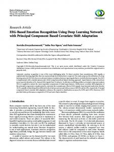
Fig. 2. Visualization of 96 filters of the first convolution layer. The filters of size 11 × 11 × 3 are learned on the 227 × 227 × 3 input images.
The network takes 227 × 227 × 3 RGB images as input. The sizes of the outputs of all the convolution layers are 55 × 55 × 96, 27 × 27 × 256, 13 × 13 × 384, 13 × 13 × 384, and 6 × 6 × 256, respectively. It is noted that the max pooling method is applied to the outputs of several convolution layers to reduce the size of the output and, thus, shorten the computation time. The output of the convolution layer is reshaped as a feature vector and fed to the fully-connected layers. After training the deep CNN, we choose the outputs of the last three layers, since these outputs of the first four layers are not discriminative enough, and the dimensions of the features are too high. To better understand the feature learned from the network, the filters of the first convolution layer are visualized in Fig. 2. The successive outputs are learned from those of the first layer, and the visualizations of such filters are abstract and difficult to find meaningful patterns. Each filter has three channels as it takes RGB image pixels as input. In Fig. 2, most filters are visualized as red, green, blue, white, and black. It reveals that the filters can obtain large response in these colors. It is noted that some edge filters, such as the half-white and half-black filters, are also learned. The discovery indicates that the edge feature may help in color classification as well. We provide a detailed discussion on this point in Section IV.
IEEE TRANSACTIONS ON INTELLIGENT TRANSPORTATION SYSTEMS
feature adopts the pooling method to combine all local features. However, the representation loses the information of some pixels ignored in the stage of pooling. Our feature describes the image in more detail since the information of each pixel in the image is considered in the feature. We choose SVM as the classifier for color classification. Based on the process of learning parameters of the convolutional layers introduced in Section III-B, the response maps of the convolutional layers are reshaped to feature vectors and fed to the successive classifier for training or testing. Selecting SVM instead of fully-connected layers (artificial neural network actually) is due to two reasons: 1) The performance of SVM is better because the regularization constraint can help combat overfitting. The problem of overfitting is regarded as a main issue of full-connected layers. 2) The number of parameters of SVM is less than that of fully-connected layers, which makes the fine-tuning procedure in training much easier. Except for the parameters of the fully-connected layers, which are able to be learned in the training step, the number of neurons, weight decay, and “dropout” ratio need to be set manually. Once the configuration of the parameters is reset, the whole deep CNN has to be retrained with a waste of much time. As features fed to SVM are the output of the pretrained deep CNN mentioned in Section III-B, the best configuration of the parameters of SVM can be tuned by cross validation, whereas the convolutional layers remain unchanged. IV. E XPERIMENTS AND D ISCUSSIONS We evaluated the proposed algorithm on a standard benchmark and compared it with other methods, including top performers in this field. All the experiments were conducted on a regular PC (3.4-GHz 8-core CPU, 8-G RAM, and Windows 64-bit OS). In testing, the process of extracting a feature from one image takes 0.187 s in the GPU mode. Moreover, the prediction by linear SVM only costs 0.0015 s, which is much less than the time spent in feature extraction. In training, learning the network takes about 5 h at 40 000 iterations. Several minutes is needed to train an SVM classifier. A. Data Set and Evaluation Measure
B. Color Recognition With SP and SVM It is common sense that the performance of image classification is superior while combined with spatial information. The SP strategy [11] is a classical method that embeds spatial information into a feature vector based on the BoW model. To the best of our knowledge, it has not been applied to the deep learning framework for the task of vehicle color recognition. The SP [11] is aimed at extracting features from different subregions and aggregating the features of all the regions together to describe an image. Unlike the feature based on BoW [11], our method computes the feature of each region in the convolutional layers in the learned CNN architecture. The BoW feature is a histogram encoded by a dictionary, whereas our feature is a set of response maps generated by the filters of the convolutional layers. To describe the image, the BoW
We assess the proposed algorithm and other methods on the Vehicle Color data set1 released in [10]. The data set contains 15 601 vehicle images covering eight color types. The images are captured roughly from the frontal view, by an HD camera with the resolution of 1920 × 1080. Each image only contains one vehicle, which is localized and cropped using a vehicle detector. The detection of vehicles is beyond the scope of this paper, since this work focuses on the recognition of vehicle color. The data set is challenging for its variability in weather condition, illumination, viewpoint, and vehicle type. For example, a significant color offset may appear in the condition of heavy haze, snow, or overexposure. Moreover, there are cars, trucks, sedans, and buses in the data set. 1 The data set is publicly available at http://mc.eistar.net/~pchen/project.html.
This article has been accepted for inclusion in a future issue of this journal. Content is final as presented, with the exception of pagination. HU et al.: VEHICLE COLOR RECOGNITION WITH SPATIAL PYRAMID DEEP LEARNING
The performances of the methods are measured by the recognition precision of each color category. The average precision (AP) is defined as the mean precision of all categories. B. Implementation Details We adopt the implementation of Caffe [43] to train the deep CNN architecture. In the feature learning stage, we construct the network with five convolution layers and three fullyconnected layers. The images are resized to 227 × 227 × 3. Then, the images are fed to the convolutional layer with 96 filters of size 11 × 11 × 3 and stride of four pixels. The outputs of the first convolution layer are modeled by a rectified linear unit (ReLU) [44], which is an approximation of f (x) = log(1 + exp(x)). It is demonstrated that training with the ReLU layer is several times faster than that in [12]. Max pooling reduces the size of the output of the ReLUs with the kernels of 3 × 3 and the stride of two pixels. Then, the output is normalized by a norm layer to ensure that the output is within a smaller range. The outputs of the first, fourth, and fifth convolutional layers are processed by pooling and normalization operations in our method. The detailed construction of the deep CNN is shown in Table I. In the fully-connected layers, the mechanism of dropout [12] is applied to alleviate overfitting. The dropout technique [12] is the most common method to reduce the influence of overfitting in training deep learning networks. The fully-connected layers can be regarded as a classifier, which is actually the artificial neural network. The first two fully-connected layers contain 4096 neurons, respectively. The number of the neurons of the last connected layer is equal to the number of the color types. When training the linear SVM classifier, we take the outputs of C5, f c6, and f c7 as the features to represent vehicle images. According to the configuration of the network to learning features, the vectors of sizes 46080, 20480, and 20480 are generated. As the output of the convolutional layer is a set of response maps, the feature of C5 can be shortened by resizing the heights and widths of the response maps. The C5 in Tables II–IV are resized into a vector with a length of 11520 by a factor of 0.5. In our experiments, we discover some redundancy in the features, and it can be reduced to smaller ones without hurting the performance. Further analysis of the redundancy will be discussed in Section IV-I. To encode spatial information, the features of different subregions of a vehicle image are also generated. The images are divided into 2 × 2 subregions. Then, the features of each subregion and the whole image are concatenated to form a long vector. The aggregated features and the corresponding labels are used to train the linear SVM classifier, which is implemented in LibLinear [45]. C. Visualization of Convolution Layer Responses To better understand the advantage of the proposed method, the response maps filtered by the first convolutional layer are visualized in Fig. 3. One of the main challenges in vehicle color recognition is to select representative ROIs on the body of the vehicle. It is reasonable to describe the color of the vehicle by its hood and roof instead of wheels, windows, headlights,
5
license plate, etc. The recent method [10] divides the image into subregions and determines the weights of each subregion by training a classifier. However, their features are the combination of conventional color histograms. The convolutional layers in our method execute convolutions with a group of filters to generate the response maps, which are also used as the features to train a classifier. The response maps of the first convolutional layer are shown in Fig. 3. The reason for selecting the first convolutional layer is that the successive layers take the response maps as input, which are more abstract and difficult to make an analysis of. In Fig. 3, it is obvious that some response maps correspond to meaningful ROIs, which are effective at distinguishing different color types. Several response maps assign the high scores to the pixels of the regions of either vehicle body or background. The reason is that the filters are learned to extract the discriminative pixels, which are informative for color classification. As shown in Fig. 3, the filters are trained to extract the red pixels due to the color of the vehicle. It is interesting that some response maps are similar with the edge of the vehicle image. It means that edge information can also benefit vehicle color recognition. D. Performance of Feature Learning Various artificial features are designed to describe the color of an image. However, the features are task independent and not necessarily effective for color recognition in certain conditions. To verify the advantage of learned features, we compared the performance of the proposed algorithm with conventional features. The compared features can be roughly separated into two classes: One class is global features, such as Color Correlogram [22] and Layered Color Indexing [46]. The features represent the color of an image as a single vector or matrix. The other class is patch features. In the comparison, several conventional patch features are chosen, such as Hue Hist [21], Normalized RG Hist [7], Opponent Hist [8], RGB Hist, Transformed Color Hist [8], and the combination of them. Our features are generated from the output of the fifth convolutional layer in the deep CNN. Here, the whole image without any subregions is used as the input of the deep CNN. To make a fair comparison, linear SVM is taken as the classifier for all the features. The performances of all the features are depicted in Table II. As can be seen from Table II, the precision of the proposed feature is clearly superior than the conventional features. Our method achieves the highest recognition accuracy on seven out of eight color classes, except for the black class. However, the precision of the black color is also very high and on par with the best score. The precision of the green color is significantly enhanced by the proposed feature. The discrimination between gray and green vehicles is more difficult, due to the large variation of these two colors. The artificial features are designed to tackle the influence of overexposure and color offset, based on the hypothesis proposed by humans. In natural scenes, particularly on urban roads, the colors of the vehicle images are complicated. Therefore, the artificial features will have difficulty covering all possible situations in complex scenarios. In contrast, the proposed feature, automatically learned from
This article has been accepted for inclusion in a future issue of this journal. Content is final as presented, with the exception of pagination. 6
IEEE TRANSACTIONS ON INTELLIGENT TRANSPORTATION SYSTEMS
TABLE II P ERFORMANCES OF A RTIFICIAL F EATURES AND D EEP CNN P RETRAINED F EATURES
TABLE III P ERFORMANCES OF SP AND SVM C LASSIFIER
TABLE IV P ERFORMANCES OF D IFFERENT L AYERS OF THE N ETWORK
raw RGB pixels, is able to handle the variations in realworld vehicle images and leads to higher recognition accuracy. Fig. 4 demonstrates several challenging vehicle images for which the proposed method gave correct predictions. As can be seen, it is robust to interference factors such as unsatisfactory illumination, haze, and dust. This confirms that automatically learned features can better adapt to various variations in realworld scenes and perform better than those designed manually. E. Performance of SP and SVM One of our main contribution is to combine spatial information with the features learned by the deep learning architecture. To verify it, we set the former top performer [10] on this data set as the baseline and compare the proposed method with it. The features of the baseline are processed by principal component analysis and coordinate augmentation. To add spatial information to the features learned by the deep learning network, we divide vehicle images into 2 × 2 subregions following the strategy of SP matching [11]. Then, the features of the subregions and the whole image are aggregated together. To enhance the performance further, SVM is used to replace the fully-connected layers since the SVM is more effective at overcoming the influence of overfitting. The performances of SP and SVM are shown in Table III. As can be seen from Table III, spatial information and SVM improve the recognition performance substantially, whereas the performance of the proposed method without spatial information and SVM classifier is still superior than the baseline. It is noted that spatial information is considered in the
method of baseline. It further proves that the features learned from the network are more informative than the artificial features. The result also confirms the conclusions in Section IV-D. Moreover, we compared the performances of SP with both fully-connected layers (SP-CNN(C5) + full) and SVM classifier (SP-CNN(C5) + SVM). SP benefits both classifiers, as shown in Table III. The performances of the outputs of the different layers in the deep architecture are listed in Table IV. As the dimensions of the outputs of the other layers are much larger but less discriminative, their precision is not evaluated. Table IV shows that the outputs of the three layers exhibit very similar results for vehicle color recognition. As the dimensions of the features of f c7 and f c6 are both 20480, the output of cn5 is a shorter feature vector of length 11520. Therefore, color recognition using the feature of cn5 is more efficient. Moreover, we have combined traditional color feature (handcrafted feature) with deep features. We have experimented with three combinations: additional color feature in [10] with C5, f c6, and f c7,, respectively. As can be seen from Table IV, the average recognition accuracies are slightly improved after incorporating an additional color feature. This indicates that deep learning features and hand-crafted features are complementary. F. Significance of Performance Difference Among Comparing Algorithms To verify that the performance gain achieved by the proposed algorithm is significant, we performed the Student’s t-test as
This article has been accepted for inclusion in a future issue of this journal. Content is final as presented, with the exception of pagination. HU et al.: VEHICLE COLOR RECOGNITION WITH SPATIAL PYRAMID DEEP LEARNING
7
Fig. 4. Vehicle color recognition examples by the proposed algorithm.
Fig. 3. Visualization of the response maps of the 96 filters in the first convolution layer. (a) Input image. (b) Response map filtered by the first convolutional layer.
and the whole set varied in the range of 0.1, 0.2, . . . , 0.9. Training/test examples were randomly selected, and the procedure was repeated five times for each group of training/test split. Three types of features, i.e., C5, f c6, f c7, were used in this experiment. The average accuracies of different groups of training/test splits are shown in Table V. As can be seen, the recognition performance consistently keeps at a high level when the ratio of training/test changes, which confirms that the ratio of training data does not influence the final recognition accuracy, for all the three types of features (C5, f c6, f c7). H. Effect of Classifier
a statistical test. We repeat out experiment ten times to obtain the AP of eight colors at each time. As the AP of comparing algorithms is the mean value of repeated independent trials, the test can be treated as a one-sample t-test. In the test, the null hypothesis is that the mean of APs of our method is equal to that of the comparing methods. We use the highest AP of the comparing algorithms, since if the improvement of our method is proved, the result of our method is also better than the other algorithms. The values of APs of our method in Table II are the mean of ten times. The standard deviations of the APs of CN5, FC6, and FC7 are 0.0065, 0.0034, and 0.0019, respectively. As a result, the p-value of the three features is 5.2967e-06, 7.1198e-08, and 2.9042e-09. The p-value is much smaller than 0.05, which is the common test p-value level. Due to the small p-value, we can evidentially reject the null hypothesis proposed before. Hence, it indicates the significance of performance difference among the comparing algorithms. G. Effect of Training/Test Ratio Here, we investigate how the vehicle color recognition accuracy varies when the training/test ratio changes. This is to examine if the ratio of training data influences the final recognition performance. We experimented with nine groups of training/test splits, where the ratio between the training data
It is widely accepted that the choice of classifier largely determines the accuracy of classification. Here, we replaced the linear SVM used in the previous experiments with an intersection kernel SVM. The performances of linear and kernel SVM are shown in Table VI. As can be observed, kernel SVM performs better than linear SVM. However, considering efficiency in training and testing, we chose linear SVM as the default classifier in practice. I. Analysis of Feature Redundancy In our experiments, the information of the response maps of the last convolutional layer is redundant for color recognition. To evaluate the extent of redundancy of the output of the convolutional layers, the response maps are resized into different scales. The convolutional layers output the features with the size of 6 × 6 × 256. We change the values of the first two dimensions and maintain the last dimension, which is equal to the number of the response maps. In our test, the values of the first two dimensions range from 1 to 12. We assess the performances of different feature sizes using the AP on the eight color types and demonstrate them in Fig. 5. The response maps at the scale of 1 are resized into one pixel. However, the features at the smallest scale still outperform the baseline in Table III. This indicates that the proposed feature is more informative than conventional features, even at an
This article has been accepted for inclusion in a future issue of this journal. Content is final as presented, with the exception of pagination. 8
IEEE TRANSACTIONS ON INTELLIGENT TRANSPORTATION SYSTEMS
TABLE V AVERAGE ACCURACIES OF D IFFERENT G ROUPS OF T RAINING /T EST S PLITS
TABLE VI P ERFORMANCES OF L INEAR AND K ERNEL SVM
Fig. 6. Failure cases. Word before bracket: predicted color type. Word in bracket: ground truth.
Fig. 5. Performances of different sizes of the feature.
extremely small scale. The performance increases with the growth of scale at small scales and gradually declines after the scale of 5. It proves that features of higher dimensions are not effective for vehicle color recognition. This reveals that there may be certain redundancy in features with higher dimensions. J. Limitation of Proposed Algorithm Although the proposed algorithm works well under various challenging conditions, it is far from perfect. It might make mistakes or give wrong predictions in certain cases. As shown in Fig. 6, a majority of the incorrect predictions are caused by severe illumination or indistinguishable colors. This means that there is still room for further improvement in vehicle color recognition. V. C ONCLUSION In this paper, we have presented a deep-learning-based algorithm for vehicle color recognition. This algorithm combines the CNN architecture with the SP strategy, which naturally captures the variations in vehicle images while making full use of the structural information of vehicles. The experiments on a standard benchmark in this field confirm that the proposed
algorithm obtains state-of-the-art performance. Moreover, it works well in various challenging situations and eliminates the necessity of preprocessing, which is a key step in previous methods. Moreover, the method proposed in this work is general and can be readily applied to other problems and domains [47]–[52]. Since the proposed method achieves very high vehicle color recognition accuracy and runs reasonably fast, we plan to integrate it into real-world applications and systems in the future. ACKNOWLEDGMENT The authors would like to thank the anonymous reviewers for their constructive comments and valuable suggestions. R EFERENCES [1] C. Anagnostopoulos, I. Anagnostopoulos, V. Loumos, and E. Kayafas, “A license plate-recognition algorithm for intelligent transportation system applications,” IEEE Trans. Intell. Transp. Syst., vol. 7, no. 3, pp. 377–392, Sep. 2006. [2] Y. Wen et al., “An algorithm for license plate recognition applied to intelligent transportation system,” IEEE Trans. Intell. Transp. Syst., vol. 12, no. 3, pp. 830–845, Sep. 2011. [3] J. B. Kim and H. J. Kim, “Efficient region-based motion segmentation for a video monitoring system,” Pattern Recognit. Lett., vol. 24, no. 1–3, pp. 113–128, Jan. 2003. [4] E. Elaad, A. Ginton, and N. Jungman, “Detection measures in reallife criminal guilty knowledge tests,” J. Appl. Psychol., vol. 77, no. 5, pp. 757–767, Oct. 1992. [5] G. S. Becker and G. J. Stigler, “Law enforcement, malfeasance, and compensation of enforcers,” J. Appl. Psychol., vol. 3, no. 1, pp. 1–18, Jan. 1974.
This article has been accepted for inclusion in a future issue of this journal. Content is final as presented, with the exception of pagination. HU et al.: VEHICLE COLOR RECOGNITION WITH SPATIAL PYRAMID DEEP LEARNING
[6] J. Zhang et al., “Data-driven intelligent transportation systems: A survey,” IEEE Trans. Intell. Transp. Syst., vol. 11, no. 4, pp. 1624–1639, Dec. 2010. [7] T. Gevers et al., “Color feature detection,” in Color Image Processing: Methods and Applications. Boca Raton, FL, USA: CRC Press, pp. 203–226, 2007. [8] K. E. Van De Sande, T. Gevers, and C. G. Snoek, “Evaluating color descriptors for object and scene recognition,” IEEE Trans. Pattern Anal. Mach. Intell., vol. 32, no. 9, pp. 1582–1596, Sep. 2010. [9] J. R. Kender, “Saturation, heu, and normalized color: Calculation, digitization effects, and use,” Carnegie Mellon Univ., Pittsburgh, PA, USA, Tech. Rep., Nov. 1976. [10] P. Chen, X. Bai, and W. Liu, “Vehicle color recognition on urban road by feature context,” IEEE Trans. Intell. Transp. Syst., vol. 15, no. 5, pp. 2340–2346, Oct. 2014. [11] S. Lazebnik, C. Schmid, and J. Ponce, “Beyond bags of features: Spatial pyramid matching for recognizing natural scene categories,” in Proc. IEEE Comput. Vis. Pattern Recog., 2006, vol. 2, pp. 2169–2178. [12] A. Krizhevsky, I. Sutskever, and G. E. Hinton, “Imagenet classification with deep convolutional neural networks,” in Proc. Adv. Neural Inf. Process. Syst., 2012, pp. 1097–1105. [13] B. Boser, I. Guyon, and V. Vapnik, “A training algorithm for optimal margin classifiers,” in Proc. COLT, 1992, pp. 144–152. [14] P. Agrawal, R. Girshick, and J. Malik, “Analyzing the performance of multilayer neural networks for object recognition,” in Proc. ECCV, 2014, pp. 329–344. [15] K. Chatfield, K. Simonyan, A. Vedaldi, and A. Zisserman, “Return of the devil in the details: Delving deep into convolutional nets,” in Proc. Brit. Mach. Vis. Conf., Nottingham, U.K., 2014, pp. 1–11. [16] S. Maji, A. C. Berg, and J. Malik, “Classification using intersection kernel support vector machines is efficient,” in Proc. IEEE Comput. Vis. Pattern Recog., 2008, pp. 1–8. [17] K. Jarrett, K. Kavukcuoglu, M. Ranzato, and Y. LeCun, “What is the best multi-stage architecture for object recognition?” in Proc. IEEE 12th Int. Conf. Comput. Vis., 2009, pp. 2146–2153. [18] G. E. Hinton and R. S. Zemel, “Autoencoders, minimum description length, and helmholtz free energy,” in Proc. Adv. Neural Inf. Process. Syst., 1994, pp. 3–10. [19] K. E. A. van de Sande, T. Gevers, and C. G. M. Snoek, “Empowering visual categorization with the GPU,” IEEE Trans. Multimedia, vol. 13, no. 1, pp. 60–70, Feb. 2011. [Online]. Available: http://www.science.uva. nl/research/publications/2011/vandeSandeITM2011 [20] P. Sermanet et al., “Overfeat: Integrated recognition, localization and detection using convolutional networks,” arXiv preprint arXiv:1312.6229, 2013. [21] J. Van De Weijer, T. Gevers, and A. D. Bagdanov, “Boosting color saliency in image feature detection,” IEEE Trans. Pattern Anal. Mach. Intell., vol. 28, no. 1, pp. 150–156, Jan. 2006. [22] J. Huang, S. R. Kumar, M. Mitra, W.-J. Zhu, and R. Zabih, “Image indexing using color correlograms,” in Proc. IEEE Comput. Vis. Pattern Recog., 1997, pp. 762–768. [23] J. Ma, J. Zhao, J. Tian, X. Bai, and Z. Tu, “Regularized vector field learning with sparse approximation for mismatch removal,” Pattern Recog., vol. 46, no. 12, pp. 3519–3532, Dec. 2013. [24] J. Ma, J. Zhao, J. Tian, A. L. Yuille, and Z. Tu, “Robust point matching via vector field consensus,” IEEE Trans. Image Process., vol. 23, no. 4, pp. 1706–1721, Apr. 2014. [25] Y.-C. Wang, C.-T. Hsieh, C.-C. Han, and K.-C. Fan, “The color identification of automobiles for video surveillance,” in Proc. IEEE ICCST, 2011, pp. 1–5. [26] M. Yang, G. Han, X. Li, X. Zhu, and L. Li, “Vehicle color recognition using monocular camera,” in Proc. IEEE Int. Conf. WCSP, 2011, pp. 1–5. [27] E. Dule, M. Gökmen, and M. S. Beratoglu, “A convenient feature vector construction for vehicle color recognition,” in Proc. 11th WSEAS Int. Conf. NN, Iasi, Romania, 2010, pp. 250–255. [28] R. Girshick, J. Donahue, T. Darrell, and J. Malik, “Rich feature hierarchies for accurate object detection and semantic segmentation,” arXiv preprint arXiv:1311.2524, 2013. [29] S. A. Eslami, N. Heess, C. K. Williams, and J. Winn, “The shape Boltzmann machine: A strong model of object shape,” Int. J. Comput. Vis., vol. 107, no. 2, pp. 155–176, Apr. 2014. [30] N. Le Roux and Y. Bengio, “Representational power of restricted Boltzmann machines and deep belief networks,” Neural Comput., vol. 20, no. 6, pp. 1631–1649, Jun. 2008.
9
[31] Y. LeCun et al., “Backpropagation applied to handwritten zip code recognition,” Neural Comput., vol. 1, no. 4, pp. 541–551, Winter 1989. [32] Y. Lecun, L. Bottou, Y. Bengio, and P. Haffner, “Gradient-based learning applied to document recognition,” Proc. IEEE, vol. 86, no. 11, pp. 2278–2324, Nov. 1998. [33] J. Deng et al., “Imagenet: A large-scale hierarchical image database,” in Proc. IEEE CVPR, 2009, pp. 248–255. [34] M. Everingham, L. Van Gool, C. K. Williams, J. Winn, and A. Zisserman, “The pascal visual object classes (VOC) challenge,” Int. J. Comput. Vis., vol. 88, no. 2, pp. 303–338, Jun. 2010. [35] M. Oquab, L. Bottou, I. Laptev, and J. Sivic, “Learning and transferring mid-level image representations using convolutional neural networks,” in Proc. IEEE Int. Conf. CVPR, 2014, pp. 1717–1724. [36] P. Sermanet and Y. Lecun, “Traffic sign recognition with multi-scale convolutional networks,” in Proc. IEEE IJCNN, 2011, pp. 2809–2813. [37] D. Ciresan, U. Meier, J. Masci, and J. Schmidhuber, “A committee of neural networks for traffic sign classification,” in Proc. IEEE IJCNN, 2011, pp. 1918–1921. [38] D. G. Lowe, “Distinctive image features from scale-invariant keypoints,” Int. J. Comput. Vis., vol. 60, no. 2, pp. 91–110, Nov. 2004. [39] N. Dalal and B. Triggs, “Histograms of oriented gradients for human detection,” in Proc. IEEE CVPR, 2005, vol. 1, pp. 886–893. [40] P. F. Felzenszwalb, R. B. Girshick, D. McAllester, and D. Ramanan, “Object detection with discriminatively trained part-based models,” IEEE Trans. Pattern Anal. Mach. Intell., vol. 32, no. 9, pp. 1627–1645, Sep. 2010. [41] D. Ritendra, D. Joshi, J. Li, and J. Wang, “Image retrieval: Ideas, influences, and trends of the new age,” ACM Comput. Surveys, vol. 40, no. 2, pp. 5:1–5:60, Apr. 2008. [42] S. Belongie, J. Malik, and J. Puzicha, “Shape matching and object recognition using shape contexts,” IEEE Trans. Pattern Anal. Mach. Intell., vol. 24, no. 4, pp. 509–522, Apr. 2002. [43] Y. Jia, “Caffe: An Open Source Convolutional Architecture for Fast Feature Embedding,” 2013. [Online]. Available: http://caffe.berkeleyvision. org/ [44] V. Nair and G. E. Hinton, “Rectified linear units improve restricted Boltzmann machines,” in Proc. 27th ICML, 2010, pp. 807–814. [45] R. E. Fan, K. W. Chang, C. J. Hsieh, X. R. Wang, and C. J. Lin, “Liblinear: A library for large linear classification,” J. Mach. Learn. Res., vol. 9, pp. 1871–1874, 2008. [46] G. Qiu and K. Lam, “Spectrally layered color indexing,” in Image and Video Retrieval. Berlin, Germany: Springer-Verlag, 2002, pp. 100–107. [47] A. Gonzalez, L. Bergasa, and J. Yebes, “Text detection and recognition on traffic panels from street-level imagery using visual appearance,” IEEE Trans. Intell. Transp. Syst., vol. 15, no. 1, pp. 228–238, Feb. 2013. [48] B. Tian, Y. Li, B. Li, and D. Wen, “Rear-view vehicle detection and tracking by combining multiple parts for complex urban surveillance,” IEEE Trans. Intell. Transp. Syst., vol. 15, no. 2, pp. 597–606, Apr. 2014. [49] Y.-W. Seo, J. Lee, W. Zhang, and D. Wettergreen, “Recognition of highway workzones for reliable autonomous driving,” IEEE Trans. Intell. Transp. Syst., vol. 16, no. 2, pp. 708–718, Apr. 2015. [50] C. Yao, X. Bai, and W. Liu, “A unified framework for multi-oriented text detection and recognition,” IEEE Trans. Image Process., vol. 23, no. 11, pp. 4737–4749, Nov. 2014. [51] X. Bai, C. Rao, and X. Wang, “Shape vocabulary: A robust and efficient shape representation for shape matching,” IEEE Trans. Image Process., vol. 23, no. 9, pp. 3935–3949, Sep. 2014. [52] X. Wang, B. Feng, X. Bai, W. Liu, and L. Latecki, “Bag of contour fragments for robust shape classification,” Pattern Recognit., vol. 47, no. 6, pp. 2116–2125, Jun. 2014.
Chuanping Hu received the Ph.D degree from Tong Ji University, Shanghai, China, in 2007. He is a Research Fellow and the Director of the Third Research Institute of the Ministry of Public Security, China. He is also a specially appointed Professor and a Ph.D. supervisor with Shanghai Jiao Tong University, Shanghai, China. He has published more than 20 papers, has edited five books, and is the holder of more than 30 authorized patents. His research interests include machine learning, computer vision, and intelligent transportation systems.
This article has been accepted for inclusion in a future issue of this journal. Content is final as presented, with the exception of pagination. 10
IEEE TRANSACTIONS ON INTELLIGENT TRANSPORTATION SYSTEMS
Xiang Bai (SM’14) received the B.S., M.S., and Ph.D. degrees from Huazhong University of Science and Technology (HUST), Wuhan, China, in 2003, 2005, and 2009, respectively, all in electronics and information engineering. He is a Professor with the School of Electronic Information and Communications, HUST. He is also the Vice Director of the National Center of AntiCounterfeiting Technology, HUST. His research interests include object recognition, shape analysis, scene text recognition, and intelligent systems.
Gengjian Xue received the Ph.D. degree in signal and information processing from Shanghai Jiao Tong University, Shanghai, China, in 2013. He is a Research Assistant with the Third Research Institute of the Ministry of Public Security, China. His research interests include computer vision, image processing, and artificial intelligence.
Li Qi received the B.S., M.S., and Ph.D. degrees from Huazhong University of Science and Technology, Wuhan, China, in 2002, 2005, and 2008, respectively, all in computer science. He is an Associate Professor and the Deputy Director of the R&D Center for the Internet of Things with the Third Research Institute of the Ministry of Public Security, China. His research interests include distributed computing for image processing, cloud computing, and pattern recognition.
Lin Mei received the Ph.D. degree from Xi’an Jiaotong University, Xi’an, China, in 2000. He is a Research Fellow. From 2000 to 2006, he was a Postdoctoral Researcher with Fudan University, Shanghai, China; the University of Freiburg, Freiburg im Breisgau, Germany; and the German Research Center for Artificial Intelligence. He is currently the Director of the Technology R&D Center for the Internet of Things with the Third Research Institute of the Ministry of Public Security, China. He has published more than 40 papers. His research interests include computer vision, artificial intelligence, and big data processing. Dr. Mei is a member of the Association for Computing Machinery.
Pan Chen received the B.S. and M.S. degrees from Central China Normal University, Wuhan, China, in 2008 and 2011, respectively. He is currently working toward the Ph.D. degree in the Media and Communication Laboratory, School of Electronic Information and Communications, Huazhong University of Science and Technology, Wuhan. His research areas include computer vision, pattern recognition, and intelligent transportation systems.