Vehicle Routing Problem: Doing it the Evolutionary Way Penousal Machado1,2, Jorge Tavares2, Francisco B. Pereira 1,2, Ernesto Costa 2 1
Instituto Superior de Engenharia de Coimbra, Quinta da Nora, 3030 Coimbra, Portugal Centro de Informática e Sistemas da Universidade de Coimbra, Polo II, 3030 Coimbra, Portugal {machado, xico, ernesto}@dei.uc.pt
[email protected] phone: +351 239790000
2
Abstract In this paper we describe three evolutionary approaches to the vehicle routing problem. In our first approach we use a standard genetic algorithm whilst in the second we use a coevolutionary model. The third approach concerns the extension of the previous ones through the inclusion of heuristics. We present and compare the experimental results achieved by the algorithms.
1
INTRODUCTION
The Vehicle Routing Problem (VRP) is a complex combinatorial optimization problem, which can be seen as a merge of two well-known problems: the Traveling Salesperson Problem (TSP) and the Bin Packing Problem (BPP). It can be described as follows: given a fleet of vehicles with uniform capacity, a common depot, and several costumer demands, find the set of routes with overall minimum route cost which service all the demands. VRP is NP-Hard, and therefore difficult to solve. The fact that VRP is both of theoretical and practical interest (due to its real world applications), explains the amount of attention given to the VRP by researchers in the past years. Due to the nature of the problem it is not viable to use exact approaches for large instances of the VRP (for instances with few nodes the branch and bound technique (Fisher, 1994) is well suited and gives the best possible solution). Most approaches to the VRP rely on heuristics and give approximate solutions to the problem (e.g. heuristic based (Clark, 1964) (Fisher, 1981) (Taillard, 1993) (Kindervater, 1997), tabu search (Rochat, 1995) (Xu, 1996) (Taillard, 1997), constraint programming (Shaw, 1998), granular tabu search (Toth, 1998), ant colony optimization (Gambardella, 1999)). There are also some applications of evolutionary computation (EC) techniques to the VRP, more specifically to some of its variants. However, when applied alone, their success is limited. This led
researchers to rely on hybrid approaches that combine the power of an EC algorithm with the use of specific heuristics (see, e.g., (Thangiah, 1995)) or to simplify the problem. One common simplification is to pre-set the number of vehicles that is going to be used in the solution (Zhu, 2000), (Louis, 1999). In this paper we present two EC approaches to an instance of the generic VRP. To our knowledge this is the first attempt to apply non-specific EC methods to the wide-ranging version of this problem (i.e., a version that does not consider any kind of simplification). Our first approach uses a standard genetic algorithm (GA), whilst in the second we resort to a coevolutionary model. Coevolutionary algorithms are an appealing and useful extension to the standard EC methods. The most important difference when considering this alternative class of algorithms is that the fitness of an individual is a function of the other individuals in the population. There are two basic classes of coevolutionary algorithms (Wiegand, 2001): •
Competitive coevolution, in which the fitness of an individual is determined by a series of competitions with other individuals. See, e.g., (Rosin, 1997) or (Jensen, 2001) as examples of this approach.
•
Cooperative coevolution, in which the fitness of an individual is determined by a series of collaborations with other individuals. Work described in (Potter, 2000) is an example of this methodology.
We follow the cooperative coevolutionary model. The paper has the following structure: in Section 2 we give a formal definition of the VRP problem and of some of its most popular variants. Section 3 comprises a description of our standard GA approach to the VRP, whilst in section 4 we describe the coevolutionary model proposed. Next, in section 5, we present the experimental results achieved with both approaches. Section 6 is devoted to the analysis of the influence of the use of heuristics when searching for good solutions. Finally in Section 7 we draw some overall conclusions.
2
THE VEHICLE ROUTING PROBLEM
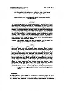
The most general version of the VRP is the Capacitated Vehicle Routing Problem (CVRP), which can be formally described in the following way. There is one central depot 0, which uses k independent delivery vehicles, with identical delivery capacity C , to service demands d i from n customers, i = 1, …, n. The vehicles must accomplish the delivery with a minimum total length cost, where the cost cij is the distance from customer i to customer j, with i, j ∈ [1, n]. The distance between customers is symmetric, i.e., cij=cji and also cii=0. A solution for the CVRP would be a partition {R1,…,Rk} of the n demands into k routes, each route Rq satisfying d p ≤ C . Associated with each R q is a permutation of p∈Rq
the demands belonging to it, specifying the delivery order of the vehicles (Ralphs, 2001). In figure 1 we present an illustration of the problem, viewed as a graph, where the nodes represent the customers. 9
Nodes
5
representing a customer node or a special blank symbol. This blank symbol acts as a separator between routes. If, in a chromosome, there are two or more consecutive blanks they are interpreted as being a single separator between two routes. Since we don’t know beforehand how many vehicles will be used in the optimal solution we must include a safe number of blank genes. Typically we set this number to the number of nodes divided by two. As genetic operators we use two standard approaches for representations involving order: the partially mapped crossover (PMX) operator and the swap mutation operator. (see, e.g., (Michalewicz, 1992) We will resort to an example in order to better describe our proposal. The chromosome presented in figure 2 codifies a solution equivalent to the one presented in figure 1. The first vehicle starts at the depot (node 0), proceeding to node 3, next to node 2, then to 7. The following gene is a blank, meaning that this vehicle won’t service any other costumers, hence returning to the depot. The next three genes in the chromosome specify the route of the second vehicle (0-8-6-5-0). Two consecutive blank genes follow this route. The next genes represent the route of the third vehicle, which is 0-4-9-1-10-0.
4
1
8 6 5 4 9 1 10 3 2 7 Figure 2: An example of a chromosome for the standard GA approach.
6
0 10
Depot 8 7 3
Routes 2
Figure 1: Vehicle Routing Problem One of the most important extensions of the CVRP is the Vehicle Routing Problem with Time Windows. This variant introduces an additional constraint type: each costumer must be served within a specific time window. Thus, at each node, the service beginning time must be greater than or equal to the beginning of the time window, and the arrival time must be lower than or equal to the end of the time window. When the arrival time is less, the vehicle has to wait. Other variants of the problem are multi-depot, fixed routes, fixed areas, etc.
3
A STANDARD GA APPROACH TO THE VRP
Our model can be viewed as an extension of the traditional GA approaches to the TSP problem. The main differences lies on the representation of the candidate solutions and their interpretation. Concerning the representation, we use a fixed size chromosome. Possible values for genes are: an integer
Some routes in the chromosome may cause the vehicle to exceed its capacity. When this happens, and to guarantee that the interpretation is always a valid candidate solution, we perform the following modification: the route that exceeds the vehicle capacity is split in several ones. Assuming that the original route is composed by the following ordered set of nodes {1, …, i, i+1, …, n}, and that the vehicle capacity is exceeded at node i+1, it will be divided in two parts: {1, …, i} and {i+1, …, n}. If necessary, further divisions can be made in the second part. Notice that these changes only occur at the interpretation level and, therefore, the information codified in the chromosome is not altered.
4
A COEVOLUTIONARY APPROACH TO THE VRP
When using cooperative coevolutionary algorithms (CCAs) the standard approach is to identify a natural decomposition of the problem into subcomponents. Each component is assigned to a subpopulation such that individuals in a given subpopulation represent potential components to the global problem. Then each component is evolved simultaneously, although isolated from the others. The only period when there is any collaboration is during the evaluation phase. In order to evaluate the fitness of a given individual, collaborators are selected from other subpopulations, so that a complete solution can be formed.
A simple algorithm of a CCA can be defined as follows: For each subpopulation S Do: Initialise population Ps (0)
the information belonging to individual B has already been distributed by the three routes. When this happens, interpretation is concluded (we already have a solution). Just like it can be confirmed there is information in chromosome A that is not necessary to obtain a solution (forth and fifth genes, in this example).
Evaluate all individuals from Ps (0) End_For
3 3 4 3 2 7 8 6 5 4 9 1 10 2 5 B A Figure 3: On the left, an individual from the first subpopulation, on the right, an individual from the second.
While termination condition not met Repeat: For each subpopulation S Do: Select a set of parents Xs(t) for next generation Apply genetic operators to individuals of Xs(t) obtaining a set of descendants Ds(t) Evaluate individuals from Ds(t) Combine P s(t) and D s(t) obtaining P s(t+1) End_For End_While Computing the fitness of an individual is the most important part of a CCA. One major question is the issue of how collaborators are chosen. Three decisions need to be considered (Wiegand, 2001): •
Collaboration pool size: number of collaborators per subpopulation to use for a given fitness evaluation.
•
Collaborator selection pressure: the degree of greediness of choosing a collaborator. How do we select individuals to collaborate? The best ones, the worst ones, in a random way?
•
Collaboration credit assignment: Given multiple collaborations, how is fitness assigned to the individual being evaluated?
In our approach we use two subpopulations. Individuals from the first subpopulation describe the number of nodes of each route, determining the size of each partition Rq. On the other hand, individuals from the second regulate the composition of each partition and also the order by which the nodes are visited. Figure 3 portrays two individuals whose joint interpretation results in a candidate solution similar to the one presented in figure 1. Individual A is from the first subpopulation, whilst individual B is from the second. The interpretation is done in the following way: the value of the first gene of individual A determines how many nodes belong to the route of the first vehicle. In this example, it has 3 nodes. Then, the first three genes from individual B specify the ordered route: {0, 3, 2, 7, 0}. Other routes are obtained in a similar way. In this situation, the route of the second vehicle has 3 nodes (as determined by the second gene from A) ordered as follows: {0, 8, 6, 5, 0} and the route of the third vehicle has 4 nodes: {0, 4, 9, 1, 10, 0}. At this point we see that
Like in the previous approach, we split routes that exceed vehicle capacity, to guarantee that the interpretation always yields a valid candidate solution. Just like we mentioned before, in the generic version of the VRP there is no way of predetermining the optimal number of vehicles, so we decided to handle this problem by setting the size of the individuals of the first subpopulation to the number of nodes divided by two. Maximum route length is also set to this value. As genetic operators, for that subpopulation, we use two-point crossover and uniform mutation (see, e.g., (Michalewicz, 1992). The size of the individuals of the second subpopulation is fixed and equal to the number of nodes. Again, we use PMX crossover and swap mutation.
5
EXPERIMENTAL RESULTS
To evaluate our approaches we tested them on an instance of the VRP from Set A of (Augerat, 1995), named A-n32k5. This instance comprises 32 nodes, with different demand values ranging from 1 to 24. The vehicle capacity is 100. The optimal solution uses five vehicles, and has a total cost of 784. 5.1
STANDARD GA APPROACH
For the results presented in this section we used the following experimental settings: population size 100, crossover rate 0.7, mutation rate 0.05, tournament selection with tournament size 5, and elitist strategy with a 5% window. We performed 30 individual runs. Each run took 1 hour of CPU time, which is, for this approach, roughly equivalent to 46500 generations. In Table 1 we summarize the results achieved, presenting the best individual found on the 30 runs and the average of the best individuals of these runs. We also present the time it took, both to find the best individual and the average of the best individuals of all runs.
Table 1: Summary of the Standard GA Results Best
Average
Cost
829
911.9
Time
3286.0
2079.6
2300
2100
1900
5.2
COEVOLUTIONARY APPROACH 1700 Cost
We used a subpopulation size of 100 and the same settings as above. Fitness was assigned as follows: for each individual of each subpopulation we chose N individuals of the other subpopulation (the pool size), one being the best of the previous generation and the others N-1 chosen randomly. The fitness of the individual is equal to the cost of the best of these candidate solutions. Results presented in this section were obtained with the following values of N: {2, 3, 5}. In table 2 we summarize the results obtained.
1500
1300
1100
900
Table 2: Summary of the coevolutionary Results
700 1
Best
10
GA
Pool Size
2
3
5
2
3
5
Cost
805
852
837
930.3
924.9
913.1
Time
252.4
319.9
3001
936.4
603.0
852.4
5.3
100 Time in seconds
1000
10000
Average
ANALYSIS OF THE RESULTS
From the experimental results presented so far one can conclude that the proposed approaches are able to reach good solutions to the VRP problem. Nevertheless, they didn’t find the optimal solution. The best individual found has an overall cost of 805, whilst the optimal solution has an overall cost of 784. It’s interesting to notice that the best individual was found using the coevolutionary approach with a pool size of 2, which were the settings that gave a worst average result. In terms of the average of the best individuals found, the standard GA and the coevolutionary approach with pool size equal to 5 gave the best results (911 and 913.1, respectively). It is also visible that in the coevolutionary approach, as the pool size increases the results tend to improve. The chart in figure 4 shows the evolution of the cost of the best individual over time (averaged from a series of 30 runs). As can be seen, on the beginning of the runs the cost drops dramatically (notice the logarithmic time scale). However after this initial drop, evolution becomes difficult. The convergence of the GA approach is slower. By looking at Tables 1 and 2 and to the time it took to find the best solution (both the overall best and average time taken) one can also conclude that the standard GA approach is the only one taking full advantage of the time assigned to each run (3600 seconds).
CE2
CE3
CE5
Figure 4: Evolution of the cost of the best individual of each generation (GA = GA approach, CEN = coevolutionary approach of pool size N). Results averaged from a series of 30 runs. A final note goes to the number of blank genes included in the chromosome of the standard approach and to the size of the individuals from the first subpopulation in the coevolutionary approach (the ones that specify routes’ length). Given that the instance being evaluated has 32 nodes, in the experiments we just described we used the value 16 for each one of the above-mentioned parameters. When we finished these tests we performed another small set of experiments with an important modification. The optimal solution for this instance requires 5 vehicles. This way we set the two parameters (blank genes in the standard GA approach and size of the chromosome of individuals from the first subpopulation in the coevolutionary model) to this value and repeated the experiments. One would expect that this might help the progress of both evolutionary algorithms. It is interesting to notice that this didn’t happen in either of the approaches. The convergence rate proved to be very high, hindering the progression of the search and resulting in worst performance.
6
IMPROVING THE RESULTS THROUGH THE USE OF HEURISTICS
The results presented so far show that the application of EC techniques to the VRP problem is promising. It is also clear that there is still room for improvement. One of the alternatives is to include some sort of heuristics in the algorithms. To test the potential of this idea we extended
the previously presented approaches by the inclusion of the K-nearest neighbor heuristic (KNN) (Mitchel, 1997), with K equal to 1. This heuristic was chosen, mostly, due to two factors: it’s a generic and simple heuristic, not specifically designed to the VRP problem; also, it’s very easy to implement and has little time complexity. The individuals are interpreted as described in Sections 3 and 4. However, when computing the cost of each route, we proceed in the following way: a)
found and overall best. In Figures 5 and 6 we present the charts of the evolution of the best individual (averaged over 30 runs), allowing to appreciate the effect of the introduction of KNN over time. It is clear from both charts that the KNN approaches perform consistently better during the entire extent of the runs. It’s interesting to notice that in the KNN coevolutionary approach the pool size doesn’t interfere with the average of the best individuals found. However, the overall best is found with pool size 2, which is also the experimental setting that has a lower computational cost.
Calculate the cost of the route based on the order expressed in the corresponding chromosome.
2500
b) Calculate the cost based on the ordering given by the KNN heuristic
2100
The cost of the route is the minimum of the costs resulting from a) and b)
This is done for each vehicle route, not for the chromosome as a whole. Thus, it’s possible to have solutions in which some vehicle routes are determined by the order expressed in the chromosome whilst others are determined by the order specified by the KNN heuristic.
1900
1700 Cost
c)
2300
1500
1300
The chromosomes can be altered to include the changes introduced during the interpretation stage, resulting in a Lamarckian evolutionary model. Alternatively these changes can be forgotten.
1100
900
700 1
10
In the following sections we will present the results achieved by the inclusion of the KNN heuristic and compare them with the previously presented ones. 6.1
GA
1000
10000
GA+KNN
Figure 5: Evolution of the cost of the best individual of each generation. Results averaged from a series of 30 runs.
EXPERIMENTAL RESULTS
Table 3 summarizes the results achieved by the genetic algorithm extended by the inclusion of the KNN heuristic, whilst Table 4 presents the same information concerning the extension of the coevolutionary approach.
1900
1700
Table 3: Summary of the GA + KNN Results Best
100 Time in seconds
Average
Cost
802
858.6
Time
3098.2
1714.0
Cost
1500
1300
1100
Table 4: Summary of the coevolutionary + KNN Results 900
Best Pool Size
2
3
Average 5
2
3
5
700 1
Cost Time
799 664.2
813 147.4
812 1081
882.3 858.8
882.8 918.0
882.0
10
100 Time in seconds
1000
10000
CE2
CE3
CE5
CE2+KNN
CE3+KNN
CE5+KNN
984.6
The comparison of these results with the previous ones shows that the addition of the KNN heuristic improves the performance of the evolutionary algorithms. This is visible both in terms of the average of the best individuals
Figure 6: Evolution of the cost of the best individual of each generation. Results averaged from a series of 30 runs.
The chart presented in Figure 7 allows the comparison of both approaches when using the KNN heuristic. In what concerns the average of the best individuals found the GA approach achieves better results (858.6 vs. approximately 882). There are also differences in terms of convergence, the GA approach converges slower, and doesn’t appear to get stuck in local optima. Like before, it takes advantage of the full extent of the run. 2500
2300
This work was partially financed by the Portuguese Ministry of Science and Technology under contract POSI/34493/SRI/2000. References Augerat, P., Belenguer, J.M., Benavent, E., Corberéan, A., Naddef, D., Rinaldi, G., Computational Results with a Branch and Cut Code for the Capacitated Vehicle Routing Problem, Research Report 949-M, Université Joseph Fourier, Grenoble, France, 1995. Clark, G., Wright, J. W., Scheduling of vehicles from a central depot to a number of delivery points, Operations Research, 12, pp. 568-581, 1964.
2100
Fisher, M. L., Jaikumur, R., A generalized assignment heuristic for vehicle routing, Network 11, pp. 109-124, 1981.
1900
Cost
1700
Fisher, M. L., Optimal solution of vehicle routing problems using minimum K-trees, Operations Research, Vol. 42, pp. 626-642, 1994.
1500
1300
Gambardella, L. M., Taillard, E., Agazzi, G., MACSVRPTW: A Multiple Ant Colony System for Vehicle Routing Problems with Time Windows , In D. Corne, M. Dorigo and F. Glover, editors, New Ideas in Optimization. McGraw-Hill, London, UK, pp. 63-76, 1999.
1100
900
700 1 GA+KNN
10
100 Time in seconds CE2+KNN
1000
CE3+KNN
10000 CE5+KNN
Figure 7: Evolution of the cost of the best individual of each generation. Results averaged from a series of 30 runs.
7
Acknowledgments
CONCLUSIONS
In this paper we presented some preliminary results concerning a comparative study among three classes of evolutionary algorithms to deal with the vehicle routing problem (VRP): the standard GA, a coevolutionary GA, and each of these algorithms enhanced by an heuristic. The VRP variant used is the most general one in the sense that the only constraint is the vehicles capacity. So there is no fixed number of vehicle or any time constraints involving the deliveries. The results achieved are promising, as they show that EC techniques can deal in a satisfactory way with the problem. In particular, we showed that the inclusion of a simple, and non-specific, heuristic to generic EC techniques provides significant improvement of the results. The characteristics of our approach suggest that it shows good scalability, allowing their application to more complex instances of the problem, where more specific techniques may fail.
Jensen, M. T., Finding Worst-Case Flexible Schedules using Coevolution, In: Proceedings of the Genetic and Evolutionary Computation Conference (GECCO-2001), p. 1144-1151, 2001. Kindervater, G. A. P., Savelsbergh, M. W. P., Vehicle routing: handling edge exchanges, E. H. Aarts, J. K. Lenstra, eds., Local Search in Combinatorial Optimization. John Wiley & Sons, Chichester, UK, pp. 311–336, 1997. Louis, S., Yin, X., Yuan, Z, Multiple Vehicle Routing with Time Windows Using Genetic Algorithms, In: Proceedings of the Congress of Evolutionary Computation, pp. 1804-1808,1999. Michalewicz, Z. Genetic Algorithms + Data Structures = Evolution Programs, Springer-Verlag, 1992. Mitchel, T., Machine Learning, McGraw-Hill, pp. 230-233, 1997. Potter, M. A., De Jong, K.. Cooperative Coevolution: An Architecture for Evolving Coadapted Subcomponents. Evolutionary Computation, 8(1), pp. 1-29. MIT Press, 2000. Ralphs, T. K., Kopman, L., Pulleyblank, W., Trotter, L. E., On the Capacitated Vehicle Routing Problem, To be published on Mathematical Programming, 2001. Rochat, Y., Taillard, É. D., Probabilistic Diversification and Intensification in Local Search for Vehicle Routing, Journal of Heuristics 1, pp. 147-167, 1995.
Rosin, C. D., Belew, R. K., New Methods for Competitive Coevolution, Evolutionary Computation, vol 5, nr 1, pp 1-29, 1997. Shaw, P., Using Constraint Programming and Local Search Methods to Solve Vehicle Routing Problems, Proceedings of the Fourth International Conference on Principles and Practice of Constraint Programming (CP '98), M. Maher and J.-F. Puget (eds.), Springer-Verlag, pp. 417-431, 1998. Taillard, É. D., Badeau, P., Gendreau, M., Guertin, F., Potvin, J.-Y., A Tabu Search Heuristic for the Vehicle Routing Problem with Soft Time Windows, Transportation Science 31, pp. 170-186,1997. Taillard, É. D., Parallel Iterative Search Methods for Vehicle Routing Problems, Networks 23, pp. 661-673, 1993. Thangiah, S. R., Vehicle routing with time windows using Genetic Algorithms, Application and Book of Genetic Algorithms: New Frontiers, Volume II. Chambers, L. (ed), pp. 253-277, CRC Press, 1995. Toth, P., Vigo, D., The Granular Tabu Search (and its Application to the Vehicle Routing Problem), Technical Report, Dipartimento di Elettronica, Informatica e Sistemistica, Università di Bologna, Italy, 1998. Wiegand, R. P., Liles, W. C., De Jong, K. A., An Empirical Analysis of Collaboration Methods in Cooperative Coevolutionary Algorithms, In Proceedings of the Genetic and Evolutionary Computation Conference (GECCO), pp. 1235–1245, Morgan Kaufmann Publishers, 2001. Xu, J., Kelly, J., A Network Flow-Based Tabu Search Heuristic for the Vehicle Routing Problem, Transportation Science 30, pp. 379-393, 1996. Zhu, K., A New Genetic Algorithm for VRPTW, International Conference on Artificial Intelligence, Las Vegas, USA, 2000.