Hindawi Publishing Corporation Mathematical Problems in Engineering Volume 2015, Article ID 506794, 10 pages http://dx.doi.org/10.1155/2015/506794
Research Article Vehicle-Scheduling Model for Operation Based on Single-Depot Jing Teng,1 Shuang Jin,2 Xiongfei Lai,1 and Sijin Chen1 1
Key Laboratory of Road and Traffic Engineering of the Ministry of Education, Tongji University, 4800 Cao’an Highway, Shanghai 201804, China 2 School of Transportation Engineering, Tongji University, 4800 Cao’an Highway, Shanghai 201804, China Correspondence should be addressed to Shuang Jin;
[email protected] Received 23 January 2015; Accepted 22 February 2015 Academic Editor: Wei (David) Fan Copyright © 2015 Jing Teng et al. This is an open access article distributed under the Creative Commons Attribution License, which permits unrestricted use, distribution, and reproduction in any medium, provided the original work is properly cited. Centralized assigning of bus running between multiple lines can save operation cost of transit agency. As more big transit terminals can serve for multiple bus lines being established, coordinating the operation of these lines’ vehicles becomes more economical and perspective. This paper proposed a vehicle-scheduling model for multiple lines which share vehicle resource together and service based on the same terminal. The optimization goal is to minimize the number of vehicles while considering reducing the invalid operation time under the constraint of timetable schemes and matching time for vehicle crossing two lines. A case in Ningbo city, China, was conducted to compare the performance of the cross-line schedules with the original schedules assigning vehicles within respective lines. The optimized schedules can reduce 7.14% vehicles in need while meeting the timetable schemes of all bus lines, which indicated that the proposed model is suitable for operation practice.
1. Introduction Vehicle-schedule is an important production plan for transit agency which assigns vehicle trips according to timetable. The quality of the vehicle-schedule is mainly shown with the number of vehicles which means that fewer vehicles used usually need lower cost. Traditionally, a vehicle only runs within a single line and could not be swapped to the other line. The average service headway of a bus line per hour usually varies in a day to meet the fluctuation of passenger demand, and the number of vehicles equipped with a bus line depends on the average departure headway in peak hour. Therefore, there are often some vehicles being surplus in off-peak hour. Comparatively, the cross-line operation mode assigning vehicles to multiple lines could save the number of vehicles and especially could be feasible to the lines whose distributions of passenger demands are staggered complementary. In addition, the cross-line scheduling can promote the efficiency of human resources and vehicle maintenance facilities. With the informatization of public transportation industry, many transit agencies have set up control centers, which have the requirement of centrally and economically dispatching vehicle resource [1]. The cross-line operation mode has a good prospect for development.
The vehicle-scheduling of cross-line operation mode is a research hotspot in applied mathematics. It could be divided into two categories: single-depot vehicle-scheduling (SDVS) and multidepot vehicle-scheduling (MDVS). The difference between them is whether the vehicle resource is assigned from single-depot to multiple lines or assigned from multiple depots to multiple lines. SDVS problem gets more attention than MDVS from the view of applicability. Bodin and Golden in 1981 presented that SDVS problem could be solved by two-phase method when setting the optimization goal as minimizing empty vehicle trip time. However, as adding the line operation time as a constraint, this problem becomes an NP hard problem and needs heuristic algorithm to solve it [2]. In 2008, Ren et al. introduced Tabu Search algorithm into genetic algorithm to solve the optimization model with the target of minimizing passenger waiting time and operating cost. This algorithm is validated that the proposed algorithm is more efficient than standard genetic algorithm, which was ever an effective method to solve the problem of bus dispatching [3]. In 2012, Wei set the model with the goal of maximizing the utilization rate of vehicles and the constraints of schedule reliability. The model was solved through the heuristic algorithm with genetic algorithm, ant colony algorithm, and particle swarm
2
Mathematical Problems in Engineering
optimization algorithm. The result indicated that operational cost and reliability have the direct proportional relationship [4]. MDVS is more complicated than SDVS and most of the research results are theoretical. Bertossi stated that the MDVS is an NP problem. In 1981, Ceder and Stern set up timetable compensation function based on the difference of actual arrival time and timetable. This method could establish the connection of the arrival time of each vehicle and start time of its first subsequent vehicle. But this method was not suitable for solving large-scale problems [5]. In 1990, Lamatsch proposed a time-space network method to solve multiproduct matching problem [6]. In the same year, Mesquita and Paixao solved a problem of multidepot vehiclescheduling problem as a multiproduct matching problem and proposed a network flow calculation method. The problem involved two cases: 2 depots with 250 trips and 3 depots with 200 trips [7]. In 1997, Lobel modified Forbes model and successfully solved a problem in Germany with 49 depots and 25000 runs and optimized thirteen million variables through the column generation technique of Lagrange pricing method to adjust linear slack time problem with multiple depots. However, his method did not consider the constraint of line operation time [8]. In 2009, Mao and Li solved transit vehicle scheduling through the general fixed job sorting algorithm, which could improve the utilization of vehicles. But the method increased the dwell time in the depot greatly [9]. In 2011, Naumann et al. presented a new robust stochastic programming method through adjusting the fixed slack time between two adjacent trips to reduce the total expected cost. This model enhanced the computation complexity so that it is only suitable for small- and medium-sized vehicle-scheduling problem [10]. As the enterprise’s operation requires high applicability, MDVS is difficult to guarantee the reliability of implementation. Relatively, SDVS is easier to manage, especially when more lines service the same terminal, because it can reduce vehicle’s invalid dwelling time for matching two trips and is convenient for the passengers to transfer through the vehicle when crossing between lines. The majority of research results widely set up nonlinear multiobject models for SDVS and adopt heuristic algorithms. In consideration of the efficiency and reliability, most of the SDVS models and algorithms cannot be applied in practice. After reviewing the previous research, this paper puts forward a method of using fixed job sorting algorithm which belongs to deterministic algorithm to solve SDVS.
2. Problem Description Figure 1 shows the cross-line operation mode based on a terminal in this paper. The background of this operation mode is as follows. (1) There are many bus terminals or intermodal transit terminals established or being planned in big cities; transit-oriented development especially based on terminals has become one tendency of urban planning in developing countries, such as China.
Line 4 Line 2 Line 3
··· Line n − 1
Line n
Line 1
The terminal shared with bus lines
The other side terminals
Figure 1: The cross-line operation mode based on a terminal.
(2) Laying out bus transit network based on terminals is beneficial for fleet management and maintenance and is also convenient for transferring organization of passenger flow. (3) Many terminals are located among functional areas to exchange passengers. Some of the lines could connect residential zones, and some could connect commercial zones or industrial zones. The peak time of the passenger volume of these lines is staggered. The transport capabilities required for these lines are complementary. (4) It is much easier for crew-scheduling based on the SDVS vehicle-scheduling than based on MDVS. Minimizing the total number of vehicles used is set as a single optimization target in this paper. Some previous researches [11] still considered another target of balancing the kilometers of all the vehicles running in a day. After the investigation of six transit agencies in China, we found that the target can be omitted because continuous rolling of the vehicles’ work during a period such as one month can easily balance the kilometers of all the vehicles. Therefore, this paper did not take the target into the objective function. The timetable schemes of each of the bus lines which set the average headway or frequency in each hour are considered as known and optimized based on passenger demands in this paper. The vehicle-scheduling results must get the trips to fit the timetable scheme of each line. Every vehicle will carry out a trip chain no matter being within one line or crossing several lines. The following constraints of the vehicle-scheduling need be confirmed. (1) Every trip of the timetable is executed. (2) Each bus can only conduct one trip at the same time. (3) Each trip can only be conducted by one bus. (4) The connecting time of two consecutive trips run by one vehicle must meet the minimal dwell time in
Mathematical Problems in Engineering
3
Table 1: The time of vehicle departing from the terminal in existing timetable (Line 9). Bus number 1 2 3 4 5 6 7 8 9 10 11 12 13 14 15 16 17 18
6:00(1) 6:07(2) 6:14(3) 6:21(4) 6:28(5) 6:35(6) 6:42(7) 6:49(8) 6:56(10) 7:03(12) 7:10(13) 7:17(15) 7:24(17) 7:30(18) 7:36(20) 7:42(21) 7:48(23) 7:54(24)
8:00(25) 8:08(27) 8:16(29) 8:24(30)
10:00(48) 10:10(49) 10:20(51)
8:32(32) 8:40(33) 8:48(35) 8:56(36) 9:04(38) 9:12(39) 9:20(41)
10:30(52) 10:40(54) 10:50(55) 11:00(57)
9:28(42) 9:36(44) 9:44(45)
11:30(61) 11:40(63)
9:52(47)
11:50(64)
11:10(58) 11:20(60)
The departure time of Line 9 in Gymnasium Station 12:00(66) 14:00(83) 16:00(106) 18:00(134) 12:10(67) 14:08(84) 16:07(108) 18:06(135) 12:20(69) 14:24(87) 16:21(112) 18:18(138) 16:28(113) 18:25(139) 14:16(86) 16:14(110) 18:12(137) 12:30(70) 14:32(89) 16:35(115) 18:32(141) 12:40(71) 14:40(90) 16:42(117) 18:39(142) 12:50(73) 14:48(91) 16:49(118) 18:46(143) 13:00(74) 15:04(94) 17:03(121) 19:00(146) 17:24(126) 19:21(150) 13:10(76) 15:12(96) 17:10(123) 19:07(147) 13:20(77) 15:20(97) 17:17(124) 19:14(148) 14:56(93) 16:56(120) 18:53(144) 13:30(78) 15:28(99) 17:30(127) 19:27(151) 13:40(80) 15:44(103) 17:42(130) 19:39(153) 17:48(131) 19:46(155) 15:36(101) 17:36(129) 19:33(152) 13:50(81) 15:52(105) 17:54(133) 19:53(156)
20:00(157) 20:10(158) 20:20(160)
22:00(174)
20:30(161) 20:40(163) 20:50(164) 21:00(165)
22:15(175) 22:30(177) 22:45(179)
21:10(167) 21:20(168) 21:30(170) 21:40(171)
21:50(172)
Note. The subscript in each cell is according to the time sequence of the timetables of Line 9 and timetables of Line 519.
the terminal which is ruled according to the basic operation works.
3. Model Building There is a premise to be stated before proposing the model that the cross-lines are equipped and run with the same type of buses in order to ensure all vehicles can serve for different bus lines. 3.1. The Mathematical Symbols. Let 𝑅 = {𝑅𝑗 | 𝑗 = 1, 2, . . . , 𝑛} be the set of cross-lines, in which 𝑗 is the serial number of bus lines and 𝑛 is the number of the bus lines to be optimized in vehicle-scheduling. Let 𝐽 = {𝐽𝑗𝑡 | 𝑗 = 1, 2, . . . , 𝑛, 𝑡 = 1, 2, . . . , 𝑦𝑗 } be the set of the whole trips departed from the terminal. 𝐽𝑗𝑡 means the 𝑡th trip of Line 𝑗. 𝑦𝑗 is the number of Line 𝑗’s trips in a day. Let 𝑃 = {𝑃𝑘 | 𝑘 = 1, 2, . . . , 𝑚} be the set of vehicles, in which 𝑘 is the serial number of vehicles and 𝑚 is the total number of vehicles. Let 𝑡𝑑𝑗𝑡 be 𝐽𝑗𝑡 ’s departure time from the terminal and let 𝑡𝑎𝑗𝑡 be 𝐽𝑗𝑡 ’s arrival time (the time back the terminal), which are determined by timetables. and 𝑡𝑗𝑡 be the upgoing running time and the Let 𝑡𝑗𝑡 downgoing running time. and 𝑡𝑡𝑗𝑡 be the dwell times of vehicle in origin Let 𝑡𝑡𝑗𝑡 station and end station. Let 𝑇𝑗𝑡 be the operational time of the trip 𝑡 of the bus line + 𝑡𝑡𝑗𝑡 + 𝑡𝑗𝑡 + 𝑡𝑡𝑗𝑡 and usually 𝑡𝑡𝑗𝑡 + 𝑡𝑡𝑗𝑡 = 15%𝑇𝑗𝑡 . 𝑗; 𝑇𝑗𝑡 = 𝑡𝑗𝑡 Let 𝐺𝑖𝑠 be the necessary time dwelling in the terminal for a vehicle connecting two consecutive trips 𝐽𝑖𝑠 and 𝐽𝑗𝑡 . 𝐺𝑖𝑠 is mainly affected by the first trip 𝐽𝑖𝑠 . Generally, its value ranges about 10%𝑇𝑖𝑠 ≤ 𝐺𝑖𝑠 ≤ 15%𝑇𝑖𝑠 .
3.2. Model Formation. With the above mathematical symbols, the model of vehicle-scheduling was built in this section. (1) Decision variable 𝑋𝑖𝑠,𝑗𝑡 𝑘 is expressed as follows: 𝑋𝑖𝑠,𝑗𝑡 𝑘
1, { { { { ={ { { { {0,
after conducting trip 𝐽𝑖𝑠 , the vehicle 𝑃𝑘 conducts trip 𝐽𝑗𝑡 ;
(1)
otherwise.
(2) Objective function is expressed as follows: the number of vehicles, running all of the trips, is 𝑍: 𝑛 𝑦𝑖 𝑛+1 𝑦𝑗 𝑘 𝑍 = 𝑃𝑘 | ∑∑ ∑ ∑𝑋𝑖𝑠,𝑗𝑡 ≥ 1, ∀𝑘 . (2) 𝑖=1 𝑠=1 𝑗=1 𝑡=1 Among them, 𝑋𝑖𝑠,(𝑛+1)𝑡 𝑘 expresses that vehicle would not conduct any trip task after conducting trip 𝐽𝑖𝑠 . Therefore, according to the principle of minimizing the number of vehicles, the objective function could be expressed as follows: 𝑛 𝑦𝑖 𝑛+1 𝑦𝑗 𝑘 min 𝑍 = 𝑃𝑘 | ∑∑ ∑ ∑𝑋𝑖𝑠,𝑗𝑡 ≥ 1, ∀𝑘 . (3) 𝑖=1 𝑠=1 𝑗=1 𝑡=1 (3) A vehicle can only conduct one trip at the same time, and then a vehicle can only conduct a follow-up trip 𝐽𝑗𝑡 after conducting trip 𝐽𝑖𝑠 . That is to say, there is a “value of 1” in the decision variable sequence 𝑋𝑖𝑠,𝑗𝑡 𝑘 for the given parameter 𝑘 and parameter 𝑖𝑠 at most: 𝑛+1 𝑦𝑗
∑ ∑𝑋𝑖𝑠,𝑗𝑡 𝑘 ≤ 1,
𝑗=1 𝑡=1
∀𝑘, 𝑖, 𝑠.
(4)
4
Mathematical Problems in Engineering Table 2: The time of vehicle departing from the terminal in existing timetable (Line 519).
Bus number 6:50(9) 21:50(173) 7:00(11) 7:10(14) 7:20(16) 7:30(19) 22:15(176) 7:45(22) 8:00(26) 22:40(178) 8:15(28) 23:05(180)
1 2 3 4 5 6 7 8
8:30(31)
The departure time of Line 519 in Gymnasium Station 10:10(50) 11:50(65) 13:30(79) 15:10(95) 16:50(119)
8:45(34)
10:30(53)
12:15(68)
9:00(37) 9:15(40)
10:50(56)
12:40(72)
9:30(43) 9:50(46)
11:10(59) 11:30(62)
13:05(75)
9 10
14:10(85) 13:50(82) 14:30(88)
14:50(92)
18:30(140)
20:10(159)
15:50(104) 15:30(100) 16:10(109) 15:20(98)
17:05(122)
18:55(145)
20:35(162)
16:30(114) 15:40(102)
17:35(128)
19:20(149)
21:00(166)
16:00(107)
17:50(132)
19:45(154)
21:25(169)
16:20(111) 16:40(116)
18:10(136)
17:20(125)
Note. The subscript in each cell is according to the time sequence of the timetables of Line 9 and Line 519.
(4) Similarly, a vehicle can only conduct a consecutive trip 𝐽𝑖𝑠 before conducting trip 𝐽𝑗𝑡 . That is to say, there is a “value of 1” in the decision variable sequence 𝑋𝑖𝑠,𝑗𝑡 𝑘 for the given parameter 𝑘 and parameter 𝑗𝑡 at most: 𝑛+1 𝑦𝑖
∑ ∑𝑋𝑖𝑠,𝑗𝑡 𝑘 ≤ 1,
∀𝑘, 𝑗, 𝑡.
(5)
𝑖=1 𝑠=1
(5) According to the principle that each trip can only be conducted by one vehicle, it can conclude that there is a “value of 1” in the decision variable sequence 𝑋𝑖𝑠,𝑗𝑡 𝑘 for the given parameter 𝐽𝑖𝑠 : 𝑚 𝑛+1 𝑦𝑗
∑ ∑ ∑𝑋𝑖𝑠,𝑗𝑡 𝑘 = 1,
∀𝑖, 𝑠.
(6)
𝑘=1 𝑗=1 𝑡=1
(6) Let 𝛽𝑘𝑗𝑡 be the matching function: {0, 𝛽𝑘𝑗𝑡 = { 1, {
the vehicle 𝑃𝑘 is matched with the trip 𝐽𝑗𝑡 ; otherwise. (7)
Therefore, according to the principle that a vehicle should be matched with a trip, the equivalent condi𝑛+1 𝑦𝑗 𝑘 tion of ∑𝑚 𝑘=1 ∑𝑗=1 ∑𝑡=1 𝑋𝑖𝑠,𝑗𝑡 = 1 is that the vehicle 𝑃𝑘 is matched with the trip 𝐽𝑗𝑡 : 𝑛+1 𝑦𝑗
∑ ∑𝑋𝑖𝑠,𝑗𝑡 𝑘 + 𝛽𝑘𝑗𝑡 ≤ 1,
∀𝑘, 𝑖, 𝑠.
(8)
𝑗=1 𝑡=1
(7) The value of the matching function 𝛽𝑘𝑗𝑡 is calculated as follows: according to the principle that the time for a vehicle connecting two consecutive trips 𝐽𝑖𝑠 and 𝐽𝑗𝑡 cannot
be smaller than 𝐺𝑖𝑠 , we could get the formulation as follows: 𝑡𝑑𝑗𝑡 𝑋𝑖𝑠,𝑗𝑡 𝑘 ≥ (𝑡𝑎𝑖𝑠 + 𝐺𝑖𝑠 ) 𝑋𝑖𝑠,𝑗𝑡 𝑘 ,
(∀𝑘, 𝑖, 𝑠, 𝑗, 𝑡) .
(9)
If the above equation holds, then 𝛽𝑘𝑗𝑡 = 0; otherwise, 𝛽𝑘𝑗𝑡 = 1.
4. Algorithm Design 4.1. Fixed Job Sorting Theory. The description of fixed job sorting algorithm: let 𝐽 = {𝐽𝑗 | 𝑗 = 1, 2, . . . , 𝑛} be the set of jobs, in which 𝑛 is the number of jobs. And the jobs in this paper correspond to bus trips. Let 𝑃 = {𝑃𝑘 | 𝑘 = 1, 2, . . . , 𝑚} be the set of processors, in which 𝑚 is the number of processors. The processors in this paper correspond to bus vehicles. Each processor can process no more than one job at the same time, and each job can be processed by no more than one processor at the same time. In addition, once a job begins to be processed, it cannot be broken off until completion of the processing. Let 𝑡𝑑𝑗 be the departure time of the fixed processing and let 𝑡𝑎𝑗 be the arrival time of the fixed processing for a job. There is a mapping function of 𝑃 → 𝐽 between a processor and a job. That is to say, there is a subset 𝑆𝑘 ∈ 𝐽 belonging to all 𝑃𝑘 ∈ 𝑃. And a processor 𝑃𝑘 could process every job belonging to 𝑆𝑘 . The key is to find a schedule to minimize the total number of processors, and all of the jobs could be processed through the mapping relationship. According to the marking method in sorting theory, the algorithm could be denoted as follows: 𝑃𝑚 | Fixed Job, 𝑃 → 𝐽
Mapping | max 𝑧 = ∑∑𝑌𝑘𝑗 , 𝑘 𝑗
(10) where 𝑃𝑚 is the number of processors, 𝑌𝑘𝑗 = 1 expresses that a processor 𝑃𝑘 conducts job 𝐽𝑗 , 𝑌𝑘𝑗 = 0 expresses that a processor 𝑃𝑘 does not conduct job 𝐽𝑗 , and max 𝑧 = ∑𝑘 ∑𝑗 𝑌𝑘𝑗
Mathematical Problems in Engineering
5 The order of departure time would be sequenced according to the timetables z1 ≤ z2 ≤ · · · ≤ zn Assign initial value of Pe , Pro(p) and Counter = 0
Supposing zx is the departure event, the corresponding trip is Jjt
Supposing zy + tis + ttis + tis as the finish event of trip Jis
Find Pk ∈ Pe satisfying the following condition:
{ me = me + 1 ) { Pe = Pe + { Pp | p = Job(is)} ) Pro(Job(is)) = m e {
{ 𝛽kjt = 0 {Pro(k) = min{Pro(p) | k ∈ P } e {
No
Judge whether Pk exists
Yes Assign Job(jt) = k, me = me − 1, Pe = Pe − {Pk } Rearrange vehicle number Pro(p) = Pro(p) − 1
{
Job(jt) = 0 Counter = Counter + 1
k= k+1
Yes
k≤n No
Stop calculating and output the value of Job(jt), jt = 1, 2, . . . , n, Counter
Figure 2: Algorithm logic diagram.
denotes the maximal number of jobs would be conducted by processors. That is to say, each job could be assigned with a processor. 4.2. Algorithm Design. The general fixed job sorting algorithm is based on first in first out (FIFO) rule to dispatch bus vehicles [9]. This paper adopts a modified fixed job sorting algorithm that the dispatching rule will assign the vehicle to conduct the trip with earlier departure time when it conforms to the requirement of minimum consecutive time in the depot, which can reduce the total operating time by compressing dwelling time in terminal. In order to describe this algorithm further, the trip is defined as Job(𝑗𝑡): 𝑝, { { { { Job (𝑗𝑡) = { { { { {0,
Trip 𝐽𝑗𝑡 conducted by bus 𝑃𝑝 (𝑝 = 1, 2, . . . , 𝑚) , Unfinished Trip.
(11)
Let 𝑃𝑒 = {𝑃𝑝 | 𝑝 = 1, . . . , 𝑚𝑒 , 𝑚𝑒 < 𝑚} be the set of all dwelling buses in terminal, in which 𝑚𝑒 refers to the amount of the dwelling buses. For each dwelling bus 𝑃𝑝 ∈ 𝑃𝑒 , which can execute trip 𝐽𝑗𝑡 , the interval between the departure time of 𝐽𝑗𝑡 and 𝑃𝑘 ’s arrival time of last trip must be longer than the necessary consecutive time 𝐺𝑖𝑠 . Therefore, for the next trip 𝐽𝑗𝑡 , a variable 𝐸 can be defined as 𝐸 = 𝑡𝑑𝑗𝑡 𝑋𝑖𝑠,𝑗𝑡 𝑘 − (𝑡𝑎𝑖𝑠 + 𝐺𝑖𝑠 ) 𝑋𝑖𝑠,𝑗𝑡 𝑘
(∀𝑘, 𝑖, 𝑠, 𝑗, 𝑡) .
(12)
Here the priority of the bus to be dispatched for the next trip is determined by the value of Pro(𝑝). Pro(𝑝) is the set of the sequence numbers depending on 𝐸. Pro(𝑝) = 1, . . . , 𝑚𝑒 , 𝑚𝑒 maps the vehicle with the biggest value of 𝐸. Here 𝛽𝑘𝑗𝑡 can be explained as {0, Bus 𝑃𝑘 is conducting trip 𝐽𝑗𝑡 , 𝛽𝑘𝑗𝑡 = { 1, otherwise. { Algorithm logic is shown as in Figure 2.
(13)
6
Mathematical Problems in Engineering Table 3: The total number of trips and vehicles.
Table 4: The 26-vehicle operation diagram.
Bus line
The total number of trips
The total number of vehicles
Line 9 Line 519 Total
126 54 180
18 10 28
Algorithm process is as follows. (1) The departure of each bus will generate a dispatching event 𝑧𝑖 which will be sorted by time series as 𝑧1 ≤ 𝑧2 ≤ ⋅ ⋅ ⋅ ≤ 𝑧𝑛 . Initializing 𝑃𝑒 , Pro(𝑝) and Counter = 0. (2) 𝑧𝑥 ∈ (𝑧1 , . . . , 𝑧𝑛 ) is defined as the departure event; the corresponding trip is 𝐽𝑗𝑡 ; then search 𝑃𝑘 ∈ 𝑃𝑒 which conforms to the constraints below: 𝛽𝑘𝑗𝑡 = 0, Pro (𝑘) = min {Pro (𝑝) | 𝑘 ∈ 𝑃𝑒 } .
(14)
If 𝑃𝑘 ∈ 𝑃𝑒 exists, then renew Job(𝑗𝑡) = 𝑘, 𝑚𝑒 = 𝑚𝑒 − 1, 𝑃𝑒 = 𝑃𝑒 − {𝑃𝑘 }. Consider 𝑃𝑝 ∈ 𝑃 and Pro(𝑝) > Pro(𝑘). Renew Pro(𝑝) = Pro(𝑝) − 1. Otherwise, renew Job (𝑗𝑡) = 0, Counter = Counter + 1.
(15)
Consider 𝑧𝑦 ∈ (𝑧1 , . . . , 𝑧𝑛 ), supposing 𝑧𝑦 +𝑡 𝑖𝑠 +𝑡𝑡𝑖𝑠 +𝑡𝑖𝑠 as the finish event of trip 𝐽𝑖𝑠 , and then 𝑚𝑒 = 𝑚𝑒 + 1, 𝑃𝑒 = 𝑃𝑒 + {𝑃𝑝 | 𝑝 = Job (𝑖𝑠)} ,
(16)
Bus label Trip chain 𝑃1 𝑃2 𝑃3 𝑃4 𝑃5 𝑃6 𝑃7 𝑃8 𝑃9 𝑃10 𝑃11 𝑃12 𝑃13 𝑃14 𝑃15 𝑃16 𝑃17 𝑃18 𝑃19 𝑃20 𝑃21 𝑃22 𝑃23 𝑃24 𝑃25 𝑃26
𝐽(1), 𝐽(25), 𝐽(48), 𝐽(66), 𝐽(83), 𝐽(106) 𝐽(2), 𝐽(27), 𝐽(49), 𝐽(68), 𝐽(85), 𝐽(105), 𝐽(132), 𝐽(155) 𝐽(3), 𝐽(28), 𝐽(51), 𝐽(69), 𝐽(89), 𝐽(114), 𝐽(136) 𝐽(4), 𝐽(30), 𝐽(93), 𝐽(120), 𝐽(144), 𝐽(164) 𝐽(5), 𝐽(103), 𝐽(130), 𝐽(153) 𝐽(7), 𝐽(33), 𝐽(98), 𝐽(122), 𝐽(145), 𝐽(175) 𝐽(9), 𝐽(31), 𝐽(50), 𝐽(86), 𝐽(110), 𝐽(137), 𝐽(159), 𝐽(173) 𝐽(10), 𝐽(36), 𝐽(56), 𝐽(70), 𝐽(88), 𝐽(108), 𝐽(135) 𝐽(6), 𝐽(32), 𝐽(53), 𝐽(67), 𝐽(84), 𝐽(109), 𝐽(131), 𝐽(154), 𝐽(171) 𝐽(12), 𝐽(37), 𝐽(54), 𝐽(72), 𝐽(87), 𝐽(112), 𝐽(138), 𝐽(160) 𝐽(8), 𝐽(107), 𝐽(133), 𝐽(156), 𝐽(172) 𝐽(14), 𝐽(35), 𝐽(55), 𝐽(75), 𝐽(92), 𝐽(113), 𝐽(139) 𝐽(15), 𝐽(40), 𝐽(57), 𝐽(74), 𝐽(94), 𝐽(121), 𝐽(146), 𝐽(166), 𝐽(178) 𝐽(11), 𝐽(34), 𝐽(52), 𝐽(71), 𝐽(90), 𝐽(116) 𝐽(17), 𝐽(111), 𝐽(134), 𝐽(157), 𝐽(174) 𝐽(13), 𝐽(41), 𝐽(60), 𝐽(77), 𝐽(97), 𝐽(125) 𝐽(18), 𝐽(42), 𝐽(61), 𝐽(78), 𝐽(99), 𝐽(129), 𝐽(152), 𝐽(170) 𝐽(20), 𝐽(44), 𝐽(63), 𝐽(80), 𝐽(102), 𝐽(124), 𝐽(148) 𝐽(16), 𝐽(38), 𝐽(101), 𝐽(128), 𝐽(149), 𝐽(166) 𝐽(21), 𝐽(45), 𝐽(64), 𝐽(82), 𝐽(100), 𝐽(126), 𝐽(150), 𝐽(168) 𝐽(23), 𝐽(46), 𝐽(62), 𝐽(77), 𝐽(96), 𝐽(123), 𝐽(147), 𝐽(167) 𝐽(19), 𝐽(39), 𝐽(59), 𝐽(73), 𝐽(91), 𝐽(119), 𝐽(140), 𝐽(158), 𝐽(176) 𝐽(24), 𝐽(47), 𝐽(65), 𝐽(79), 𝐽(95), 𝐽(118), 𝐽(143) 𝐽(26), 𝐽(115), 𝐽(141), 𝐽(161), 𝐽(177) 𝐽(22), 𝐽(43), 𝐽(58), 𝐽(81), 𝐽(104), 𝐽(127), 𝐽(151), 𝐽(169), 𝐽(180) 𝐽(29), 𝐽(117), 𝐽(153), 𝐽(163), 𝐽(179)
Pro (Job (𝑖𝑠)) = 𝑚𝑒 . (3) Renew 𝑘 = 𝑘 + 1. If 𝑘 ≤ 𝑛, the process returns to step (2); otherwise, output Job(𝑗𝑡), 𝑗𝑡 = 1, 2, . . . , 𝑛, Counter.
5. Case Study 5.1. Overview of Case. Two tested bus lines, Line 9 and Line 519 in Ningbo, China, are shown below, which share the identical terminal—Gymnasium Station. The layout of the bus lines is shown as in Figure 3. The running time of Line 9 is 51 min. The normal time for vehicles dwelling at the terminal accounts for 15% of the running time and should not be less than 10%. There are totally 126 trips conducted by 18 vehicles every day and the time of vehicle departing from the terminal in existing timetable is shown in Table 1. Similarly, the running time of Line 519 is 42 min. Therefore, the normal time for vehicles dwelling at the terminal is 8 min while the minimum dwelling time cannot be less than 5 min. There are 54 trips conducted by 10 vehicles every day
and the time of vehicle departing from the terminal in the existing timetable is shown in Table 2. The total trips and vehicles of two lines are shown in Table 3. 5.2. The Optimized Vehicle-Schedule. With the modified fixed job sorting algorithm, the cross-line vehicle-schedule can be quickly gotten and all the trips are burdened with 26 vehicles. Compared with the operation mode of single line, the method could reduce 2 vehicles which occupy 7.1% of the existing vehicle number. Table 4 shows the trip chains of the 26 vehicles in a day. Figure 4 is the operation diagram of the two bus lines under cross-line operation mode. Table 5 shows the optimized cross-line vehicle-schedule in Gymnasium Station. It is known that during the transition phase from peak period to off-peak period, the transport capacity offered in peak period will be cut away to fit with off-peak transport demand. With the modified fixed job sorting algorithm, some vehicles could get a long nonservice
A.T.1 S.T.1. D.T.2 A.T.2 S.T.2 D.T.3 A.T.3 S.T.3 D.T.4 A.T.4 S.T.4 8:22 8 8:30 10:02 8 10:10 11:42 Nonservice time 8:26 6 8:32 10:23 7 10:30 12:02 8 12:10 14:01 7 8:40 Nonservice time 9:02 10 9:12 11:03 7 11:10 12:42 8 12:50 14:41 7 9:15 Nonservice time 8:33 7 8:40 10:31 Nonservice time 9:08 7 9:15 10:47 13 11:00 12:51 9 13:00 14:51 13 9:32 Nonservice time 10:07 Nonservice time 9:17 13 9:30 11:02 8 11:10 13:01 41 13:50 15:41 9 7:58 10 8:08 9:59 11 10:10 12:01 14 12:15 13:47 13 8:54 6 9:00 10:32 8 10:40 12:31 9 12:40 14:12 12 8:12 12 8:24 10:15 Nonservice time 8:52 12 9:04 10:55 Nonservicetime 9:39 11 9:50 11:22 8 11:30 13:02 8 13:10 15:01 11 9:33 11 9:44 11:35 15 11:50 13:41 9 13:50 15:22 8 9:21 7 9:28 11:19 11 11:30 13:21 9 13:30 15:21 7 8:05 10 8:15 9:47 33 10:20 12:11 9 12:20 14:11 13 8:47 9 8:56 10:47 13 10:50 12:22 8 12:30 14:21 9 8:42 8 8:48 10:39 11 10:50 12:41 24 13:05 14:37 13 11:50 13:22 8 13:30 15:02 8 9:45 7 9:52 11:43 7 9:27 9 9:36 11:27 13 11:40 13:31 9 13:40 15:31 9 8:19 Nonservice time 7:51 9 8:00 9:51 9 10:00 11:51 9 12:00 13:51 9 8:32 13 8:45 10:17 13 10:30 12:21 19 12:40 14:31 9 9:01 19 9:20 11:11 9 11:20 13:11 9 13:20 15:11 9
D.T.5 A.T.5 S.T.5 D.T.6 A.T.6 S.T.6 D.T.7 A.T.7 S.T.7 D.T.7 A.T.7 S.T.7 D.T.7 A.T.7 14:16 16:07 7 16:14 18:05 7 18:12 20:03 7 20:10 21:42 8 21:50 23:22 14:08 15:59 11 16:10 17:42 6 17:48 19:39 6 19:45 21:17 23 21:40 23:31 16:00 17:32 22 17:54 19:45 8 19:53 21:44 6 21:50 23:41 14:48 16:39 11 16:50 18:22 8 18:30 20:02 8 20:10 22:01 14 22:15 23:47 16:20 17:52 8 18:00 19:51 9 20:00 21:51 9 22:00 23:51 15:20 16:52 13 17:05 18:37 18 18:55 20:27 8 20:35 22:07 8 22:15 0:06 15:04 16:55 8 17:03 18:54 6 19:00 20:51 9 21:00 22:32 8 22:40 0:12 16:35 18:26 6 18:32 20:23 7 20:30 22:21 9 22:30 0:21 16:42 18:33 6 18:39 20:30 10 20:40 22:31 14 22:45 0:36 15:50 17:22 8 17:30 19:21 6 19:27 21:18 7 21:25 22:57 8 23:05 0:37 14:10 15:42 10 15:52 17:43 7 17:50 19:22 24 19:46 21:37 Nonservice time 14:24 16:15 6 16:21 18:12 6 18:18 20:09 11 20:20 22:11 Nonservice time 14:56 16:47 9 16:56 18:47 6 18:53 20:44 6 20:50 22:41 Nonservice time 15:36 17:27 8 17:35 19:07 13 19:20 20:52 8 21:00 22:51 Nonservice time 15:12 17:03 7 17:10 19:01 6 19:07 20:58 12 21:10 23:01 Nonservice time 15:30 17:02 22 17:24 19:15 6 19:21 21:12 8 21:20 23:11 Nonservicetime 15:28 17:19 17 17:36 19:27 6 19:33 21:24 6 21:30 23:21 Nonservice time 14:32 16:23 7 16:30 18:02 8 18:10 19:42 Nonservice time 14:30 16:02 5 16:07 17:58 8 18:06 19:57 Nonservice time 14:50 16:22 6 16:28 18:19 6 18:25 20:16 Nonservice time 15:10 16:42 7 16:49 18:40 6 18:46 20:37 Nonservice time 15:40 17:12 5 17:17 19:08 6 19:14 21:05 Nonservice time 15:44 17:35 7 17:42 19:33 6 19:39 21:30 Nonservice time 14:00 15:51 9 16:00 17:51 Nonservice time 14:40 16:31 9 16:40 18:12 Nonservice time 15:20 17:11 9 17:20 18:52 Nonservice time
D.T., A.T., and S.T. are the abbreviations of departure time, arrival time, and dwelling time; the unit of S.T. is min.
Bus D.T.1 7 6:50 9 6:35 11 6:49 22 7:30 15 7:24 6 6:42 13 7:17 24 8:00 26 8:16 25 7:45 2 6:07 10 7:03 4 6:21 19 7:20 21 7:48 20 7:42 17 7:30 3 6:14 8 6:56 12 7:10 23 7:54 18 7:36 5 6:28 1 6:00 14 7:00 16 7:10
Table 5: The optimized cross-line vehicle-schedule of the Gymnasium Station terminal.
Mathematical Problems in Engineering 7
D.T.1 6:00 6:07 6:14 6:21 6:28 6:35 6:42 6:49 6:50 6:56 7:00 7:03 7:10 7:10 7:17 7:20 7:24 7:30 7:30 7:36 7:42 7:45 7:48 7:54 8:00 8:16
A.T.1 7:51 7:58 8:05 8:12 8:19 8:26 8:33 8:40 8:22 8:47 8:32 8:54 9:01 8:42 9:08 8:52 9:15 9:21 9:02 9:27 9:33 9:17 9:39 9:45 9:32 10:07
S.T.1 9 10 10 12 11 14 15 16 10 17 13 21 19 18 22 20 21 29 26 25 37 27 31 35 28 23
D.T.2 8:00 8:08 8:15 8:24 8:30 8:40 8:48 8:56 8:32 9:04 8:45 9:15 9:20 9:00 9:30 9:12 9:36 9:50 9:28 9:52 10:10 9:44 10:10 10:20 10:00 10:30
A.T.2 9:51 9:59 9:47 10:15 10:02 10:31 10:39 10:47 10:23 10:55 10:17 10:47 11:11 10:32 11:02 11:03 11:27 11:22 11:19 11:43 12:01 11:35 11:42 12:11 11:51 12:02
S.T.2 49 51 43 45 48 49 51 53 47 55 53 63 64 58 58 67 73 68 61 77 69 65 68 79 74 78
D.T.3 10:40 10:50 10:30 11:00 10:50 11:20 11:30 11:40 11:10 11:50 11:10 11:50 12:15 11:30 12:00 12:10 12:40 12:30 12:20 13:00 13:10 12:40 12:50 13:30 13:05 13:20
A.T.3 12:31 12:41 12:21 12:51 12:22 13:11 13:21 13:31 13:01 13:41 12:42 13:22 13:47 13:02 13:51 14:01 14:12 14:21 14:11 14:51 15:01 14:31 14:41 15:02 14:37 15:11
S.T.3 79 69 69 77 78 73 69 69 69 67 78 70 63 74 65 63 60 59 59 45 39 49 49 42 51 39
D.T.4 13:50 13:50 13:30 14:08 13:40 14:24 14:30 14:40 14:10 14:48 14:00 14:32 14:50 14:16 14:56 15:04 15:12 15:20 15:10 15:36 15:40 15:20 15:30 15:44 15:28 15:50
A.T.4 15:22 15:41 15:21 15:59 15:31 16:15 16:02 16:31 15:42 16:39 15:51 16:23 16:22 16:07 16:47 16:55 17:03 17:11 16:42 17:27 17:12 16:52 17:02 17:35 17:19 17:22
D.T., A.T., and S.T. are the abbreviations of departure time, arrival time, and dwelling time; the unit of S.T. is min.
Bus 1 2 3 4 5 6 7 8 9 10 11 12 13 14 15 16 17 18 19 20 21 22 23 24 25 26
S.T.4 38 26 31 21 29 15 19 11 28 10 23 17 13 21 9 10 14 9 8 9 12 11 8 7 11 13
D.T.5 16:00 16:07 15:52 16:20 16:00 16:30 16:21 16:42 16:10 16:49 16:14 16:40 16:35 16:28 16:56 17:05 17:17 17:20 16:50 17:36 17:24 17:03 17:10 17:42 17:30 17:35
A.T.5 17:51 17:58 17:43 17:52 17:32 18:02 18:12 18:33 17:42 18:40 18:05 18:12 18:26 18:19 18:47 18:37 19:08 18:52 18:22 19:27 19:15 18:54 19:01 19:33 19:21 19:07
S.T.5 9 12 11 14 16 10 13 20 8 20 13 18 20 13 20 18 25 22 17 19 24 26 20 20 24 20
D.T.6 18:00 18:10 17:54 18:06 17:48 18:12 18:25 18:53 17:50 19:00 18:18 18:30 18:46 18:32 19:07 18:55 19:33 19:14 18:39 19:46 19:39 19:20 19:21 19:53 19:45 19:27
Table 6: The general cross-line vehicle-schedule based on first in first out (FIFO) rule in Gymnasium Station. A.T.6 19:51 19:42 19:45 19:57 19:39 20:03 20:16 20:44 19:22 20:51 20:09 20:02 20:37 20:23 20:58 20:27 21:24 21:05 20:30 21:37 21:30 20:52 21:12 21:44 21:17 21:18
S.T.6 D.T.7 A.T.7 39 20:30 22:21 28 20:10 21:42 35 20:20 22:11 38 20:35 22:07 31 20:10 22:01 47 20:50 22:41 44 21:00 22:32 56 21:40 23:31 38 20:00 21:51 59 21:50 23:41 51 21:00 22:51 38 20:40 22:31 53 21:30 23:21 47 21:10 23:01 62 22:00 23:51 53 21:20 23:11 81 22:45 0:36 70 22:15 0:06 55 21:25 22:57 Nonservice time 95 23:05 0:37 58 21:50 23:22 63 22:15 23:47 Nonservice time 73 22:30 0:21 82 22:40 0:12
8 Mathematical Problems in Engineering
Mathematical Problems in Engineering
9
30.0 Time (min)
Gymnasium Station
32.7 min 26 vehicles
35.0
26 vehicles
25
25.0
20
20.0
15
15.0 7.9 min
10.0
10 5
5.0
0
0.0 The conjunct terminal Line 519 Line 9
30 Number (vel.)
North District Meixu Station
Center Hospital Station
Cross-line scheduling used the general algorithm
Cross-line scheduling used the modified algorithm
The average interval between two consecutive trips The number of vehicles
Figure 3: The layout of Line 9 and Line 519 in Ningbo city, China.
Figure 5: The comparison of the average intervals between two consecutive trips of two circumstances.
Line 9
6. Conclusion
Line 519
6:00 7:00 8:00 9:00 10:00 11:00 12:00 13:00 14:00 15:00 16:00 17:00 18:00 19:00 20:00 21:00 22:00 23:00 0:00
0
Figure 4: Vehicle operation diagram (all kinds of vehicles are represented by different colors).
interval (the bold italic font parts in Table 5) and others continue operating efficiently, which is beneficial for making the work plan of repairing and maintaining vehicles while rolling vehicles to execute the vehicle schedule. During the long nonservice interval, vehicles will exit operation and the bold italic font parts do not belong to the operating time, so the modified method can reduce the total operating time of the vehicles. In this case, through optimization, the total dwelling time at the terminal of 26 buses conducting 180 round trips is 1409 min. The average interval between two consecutive trips is 7.9 min. In comparison, the general fixed job sorting algorithm selects the bus vehicle to fit a connective trip based on first in first out (FIFO) rule. During the transition phase from peak period to off-peak period the vehicles that arrived earlier have to continue conducting the subsequent trips and the total vehicles’ extended dwelling time in terminal cannot be concentrated on part vehicles and then cannot be utilized for vehicle maintenance or other purposes, so the time is idle but still belongs to operating time. Table 6 shows the general cross-line vehicle-schedule based on first in first out (FIFO) rule in Gymnasium Station. In this case, with the general fixed job sorting algorithm, the total number of vehicles optimized is still 26 buses, but the total dwelling time at the terminal is 5880 min and the average interval between two consecutive trips is 32.7 min. That is the reason why we modify the general fixed job sorting algorithm. Figure 5 shows the comparison of two circumstances.
This paper studied a model to optimize cross-line vehicle scheduling for single-depot, whose optimization goal is minimizing the total number of vehicles used. Setting the sole goal avoids the complexity and uncertainty of solving the multiobjective problem and still keeps availability. The modified fixed job sorting algorithm is designed, which can not only get the deterministic optimum solution to reduce total vehicle used but also save the vehicles’ operating time. The algorithm can be easily written into computer program and the computation time is short, which is feasible for application. In fact, the vehicle-scheduling method would not be limited in bus transit operation and could be generalized to the similar scenario of logistics transport.
Conflict of Interests The authors declare that there is no conflict of interests regarding the publication of this paper.
Acknowledgment This work was supported by the National Natural Science Foundation of China (Grant no. 61174185).
References [1] J. Teng and X. G. Yang, “The study of transit coordination dispatching mode for big cities,” in Public Transport and Urban Development Studies and Practices, pp. 20–28, 2006, (Chinese). [2] L. Bodin and B. Golden, “Classification in vehicle routing and scheduling,” Networks, vol. 11, no. 2, pp. 97–108, 1981. [3] C. X. Ren, Y. J. Xun, and C. C. Yin, “Research on vehicle scheduling based on genetic tabu search algorithm,” Journal of Shandong University of Science and Technology (Natural Science Edition), pp. 53–56, 2008. [4] M. Wei, The model and algorithm of regional vehicle scheduling under uncertain information environment [Ph.D. thesis], South China University of Technology, Guangzhou, China, 2012, (Chinese).
10 [5] A. Ceder and H. I. Stern, “Deficit function bus scheduling with deadheading trip insertion for fleet size reduction,” Transportation Science, vol. 15, no. 4, pp. 338–363, 1981. [6] A. Lamatsch, “An approach to vehicle scheduling with depot capacity constraints,” in Computer-Aided Transit Scheduling: Proceedings of the 5th International Workshop on ComputerAided Scheduling of Public Transport held in Montr´eal, Canada, August 19–23, 1990, vol. 386 of Lecture Notes in Economics and Mathematical Systems, pp. 181–195, Springer, Berlin, Germany, 1992. [7] M. Mesquita and J. Paixao, “Multiple depot vehicle scheduling problem: a new heuristic based on quasi-assignment algorithm,” in Proceedings of the 5th International Workshop on Computer-aided Scheduling of Public Transit, Montreal, Canada, 1990. [8] A. Lobel, “Solving large-scale multiple-depot scheduling problems,” in Proceedings of the 7th International Conference on Computer-Aided Scheduling of Public Transit, Cambridge, Mass, USA, 1997. [9] L. Mao and W. Q. Li, “Research on transit vehicle scheduling model and its algorithm,” Journal of Transportation Systems Engineering and Information, vol. 7, no. 3, pp. 64–68, 2009 (Chinese). [10] M. Naumann, L. Suhl, and S. Kramkowski, “A stochastic programming approach for robust vehicle scheduling in public bus transport,” Procedia—Social and Behavioral Sciences, vol. 20, pp. 826–835, 2011. [11] B. Z. Lou, Research on optimization algorithm of vehicle scheduling based on deficit function [M.S. thesis], Beijing Jiaotong University, Beijing, China, 2011, (Chinese).
Mathematical Problems in Engineering
Advances in
Operations Research Hindawi Publishing Corporation http://www.hindawi.com
Volume 2014
Advances in
Decision Sciences Hindawi Publishing Corporation http://www.hindawi.com
Volume 2014
Journal of
Applied Mathematics
Algebra
Hindawi Publishing Corporation http://www.hindawi.com
Hindawi Publishing Corporation http://www.hindawi.com
Volume 2014
Journal of
Probability and Statistics Volume 2014
The Scientific World Journal Hindawi Publishing Corporation http://www.hindawi.com
Hindawi Publishing Corporation http://www.hindawi.com
Volume 2014
International Journal of
Differential Equations Hindawi Publishing Corporation http://www.hindawi.com
Volume 2014
Volume 2014
Submit your manuscripts at http://www.hindawi.com International Journal of
Advances in
Combinatorics Hindawi Publishing Corporation http://www.hindawi.com
Mathematical Physics Hindawi Publishing Corporation http://www.hindawi.com
Volume 2014
Journal of
Complex Analysis Hindawi Publishing Corporation http://www.hindawi.com
Volume 2014
International Journal of Mathematics and Mathematical Sciences
Mathematical Problems in Engineering
Journal of
Mathematics Hindawi Publishing Corporation http://www.hindawi.com
Volume 2014
Hindawi Publishing Corporation http://www.hindawi.com
Volume 2014
Volume 2014
Hindawi Publishing Corporation http://www.hindawi.com
Volume 2014
Discrete Mathematics
Journal of
Volume 2014
Hindawi Publishing Corporation http://www.hindawi.com
Discrete Dynamics in Nature and Society
Journal of
Function Spaces Hindawi Publishing Corporation http://www.hindawi.com
Abstract and Applied Analysis
Volume 2014
Hindawi Publishing Corporation http://www.hindawi.com
Volume 2014
Hindawi Publishing Corporation http://www.hindawi.com
Volume 2014
International Journal of
Journal of
Stochastic Analysis
Optimization
Hindawi Publishing Corporation http://www.hindawi.com
Hindawi Publishing Corporation http://www.hindawi.com
Volume 2014
Volume 2014