Vehicular pollution modeling using artificial neural network ... - NOPR

Journal of Scientific & Industrial Research Vol. 64, September 2005, pp. 637-647

Vehicular pollution modeling using artificial neural network technique: A review N Sharma 1,*, K K Chaudhry 2 and C V Chalapati Rao

3

1

Traffic Engineering and Transportation Planning Area, Central Road Research Institute, New Delhi 110 020 2 Department of Applied Mechanics, Indian Institute of Technology, Delhi 110 016 3 Air Pollution Control Division, National Environmental Engineering Research Institute, Nagpur 440 020 Received 19 October 2004, revised 24 May 2005; accepted 28 June 2005

Air quality models form one of the most important components of an urban air quality management plan. An effective air quality management system must be able to provide the authorities with information on the current and likely future trends, enabling them to make necessary assessments regarding the extent and type of the air pollution control management strategies to be implemented throughout the area. Various statistical modeling techniques (regression, multiple regression and time series analysis) have been used to predict air pollution concentrations in the urban environment. These models calculate pollution concentrations due to observed traffic, meteorological and pollution data after an appropriate relationship has been obtained empirically between these parameters. Recently, statistical modeling tool such as artificial neural network (ANN) is increasingly used as an alternative tool for modeling the pollutants from vehicular traffic particularly in urban areas. In the present paper, a review of the applications of ANN in vehicular pollution modeling under urban condition and basic features of ANN and modeling philosophy, including performance evaluation criteria for ANN based vehicular emission models have been described. Keywords: Air quality management, Vehicular pollution modeling, Artificial neural networks, Multilayer perceptron, Training data, Supervised learning IPC Code: G 10 K 11/ 00, G 06 N 3 / 02

Introduction Artificial Neural Networks (ANNs) began with the pioneering work of McCulloch & Pitts1 and has its root in rich interdisciplinary history from the early 1940s. Hebbs2 proposed a learning scheme for updating synaptic strength between neurons. His famous ‘postulate of learning’, which is referred to as ‘Hebbian learning’ rule, stated that the information can be stored in synaptic connections and the strength of a synapse would increase by the repeated activation of neurons by the other ones across that synapse. Rosenblatt3 and Block et al4 proposed a neuron like element called ‘perceptron’ and provided learning procedure for them. They further developed ‘perceptron convergence procedure’ which is advancement over the ‘Hebb rule’ for changing synaptic connection. Minsky & Peppert5 demonstrated limitations of the single layer perceptron. Nileson6 showed that the Multilayer Perceptrons (MLP) can be used to separate pattern nonlinearly in a hyperspace and the perceptron convergence theorem applies only ___________ *Author for correspondence Tel: 011-26847138; Fax: 011-26845943/ 26830480 Email: Sharmaniraj1990@ rediffmail.com

in single layer perceptron. Rumelhart et al7 presented the conceptual basis of back – propagation, which can be considered as a giant step forward as compared to its predecessor, perceptron. Flood & Kartem8,9 reviewed various applications in civil engineering. Dougherty10 reviewed application of ANN in transportation engineering. Godbole11 reviewed applications of ANN in wind engineering and reported two separate studies12,13, in which ANN technique simulated experimental results obtained during wind tunnel studies to determine wind pressure distribution in low buildings. Gardner & Dorling14 reviewed applications of ANN in atmospheric sciences and concluded that the neural networks generally give as good or better results than linear methods. Basic Features of ANN Biological Neuron

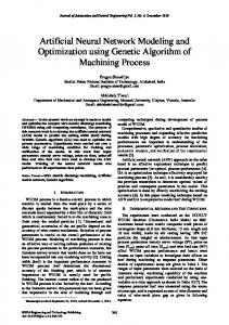
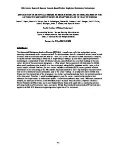
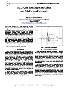
A human brain consists of a large number of computing elements (1011) called ‘neurons’ which are the fundamental units of the biological nervous system (Fig. 1). It is a simple processing unit, which receives and processes the signal from other neurons through its path called ‘dendrites’. An activity of

J SCI IND RES VOL. 64 SEPTEMBER 2005

638

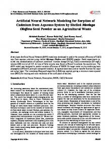
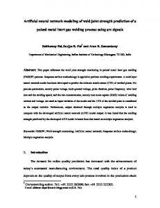
to as input to the nodes in next layer of the network implying a direction of information processing. Hence, MLP is also known as a feed-forward neural network17. Input layer passes input vector to the network. MLP can approximate any smooth measurable action between the input and output vectors16. An MLP has the ability to learn through training, which requires a set of training data consisting of a series of input and associated output vectors. Transfer Function

Fig.1 Biological neuron

Fig. 2Multilayer perceptron (MLP)

neuron is an all - or - none process i.e., it is a binary number type of process. If the combined signal is strong enough, only then it generates the output signal, which is transmitted through axon to a junction referred to as ‘synapse’. The signals, as they pass through the network, create different levels of activation in the neurons. Amount of signals transferred depends upon the synaptic strength of junction. Synaptic strength is modified during learning processes of the brain. Therefore, it can be considered as a memory unit of each inter-connection. Identification or recognition depends on the activation levels of neurons. Multilayer Perceptron

Multilayer ANN or MLP (Fig. 2) consists of a system of layered interconnected ‘neurons’ or ‘nodes’, which are arranged to form three layers: an ‘input’ layer, one or more ‘hidden’ layers, and an ‘output’ layer, with nodes in each layer connected to other nodes in neighboring layers15,16. The output of a node is scaled by connecting weights and fed forward

In ANN, each node has a set signal function that produces output, which either goes to a number of other nodes in network or to the output of the entire network. The transfer function is the mechanism of translating input signals to output signals for each processing element18. The three main types of transfer or activation functions are linear, threshold and sigmoid functions. Linear function produces an output signal in the node that is directly proportional to the activity level of node. Threshold function produces an output signal that is constant until a certain level is reached and then output changes to a new constant level until the level of activity drops back below the threshold. Sigmoid function produces an output that varies continually with the activity level but it is not a linear variation. Sigmoid transfer function has a graph similar to stretched S and consists of two functions Hyperbolic (values between –1 to +1); and logistic function (values between 0 and 1). Superposition of various non - linear transfer functions enables MLP to approximate behavior of non - linear functions. If transfer function was linear, MLP would not be able to model non – linear interactions between various variables. Sigmoid transfer function (particularly logistic function) is the most commonly used transfer function in air pollution modeling14,19. Training a MLP – the Back - Propagation Algorithm

A ‘learning’ process or ‘training’ forms interconnections (correlations) between neurons. Learning algorithm in a neural network specifies the rules or procedures that tell a node in ANN as to how to modify its weight distribution in response to input pattern. During the training, MLP is repeatedly presented with training data, and weights in network are adjusted until desired input-output mapping occurs14,18-20. ANN can be trained by ‘supervised’ or ‘unsupervised learning’. In supervised learning, external prototypes are used as target outputs for

SHARMA et al: VEHICULAR POLLUTION MODELING USING ARTIFICIAL NEURAL NETWORK TECHNIQUE

639

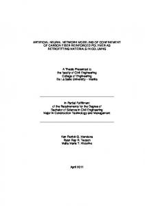
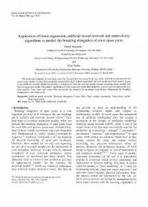
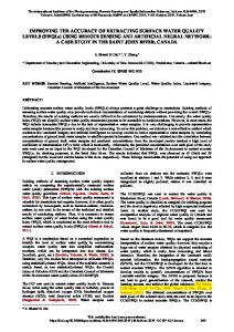
Fig. 3Schematic diagram showing the neural network training by the back -propagation algorithm

specific inputs and network is given a learning algorithm to follow and calculate new connection ‘weights’ that bring output closer to the target output. In unsupervised learning (similar to learning by students without teacher), the desired response is not known, thus explicit error information cannot be used to improve network behavior18. Thus, supervised learning involves providing samples of the input patterns that the network needs to learn and also the output patterns that the network needs to produce when it encounters those patterns. Unsupervised learning involves providing the network with input patterns, but not the desired output patterns. MLPs learn in supervised manner21,22. During training of MLP, output corresponding to given input vector may not reach the desired level. During training, magnitude of the error signal, defined as the difference between the desired and actual output, is used to determine to what degree the weights in the network should be adjusted so that the overall error can be reduced to the desired (acceptable) level. Back-propagation is a supervised learning model and is the most widely used learning method employed by training of MLP20. Generally, back-propagation learning algorithm applies in two basic steps: (i) Feed-forward calculation; and (ii) Error back propagation calculation. The inputs are fed into the input layer and get multiplied by interconnection weights as they are passed from the input layer to the first hidden layer.

Within the first hidden layer, they get summed and then processed by a nonlinear function. As the processed data leaves the first hidden layer, again it gets multiplied by interconnection weights, then summed and processed by the second hidden layer. Finally, the data is multiplied by interconnection weights and then processed one last time within the output layer to produce ANN output. With each presentation, output of ANN is compared to the desired output and an error, measured as mean square error7, is computed. This error is then fed back (back propagated) to ANN and used to adjust the weights such that error decreases with each iteration, and neural model gets closer and closer to producing the desired output (Fig. 3). The training cycle is continued until the network achieves desired level of tolerance23. Properly trained back-propagation networks tend to give reasonable answers when presented with inputs that the network has never seen before. This way, it is used as an effective prediction model for a variety of problems including air pollution - related phenomena. Feed Forward Computation

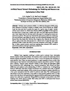
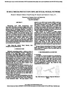
Input vector (representing patterns to be recognized) is incident on the input layer and distributed to subsequent hidden layers and finally to output layer via weighted connections (Fig. 4). Each neuron in the network operates by taking sum of its weighted input and passing the result through a non-

J SCI IND RES VOL. 64 SEPTEMBER 2005

640

Fig. 4Configuration of multilayer perceptron (MLP)

linear activation function. The net input to hidden unit is described as: n

NETpj = ∑W ji Ii +ψ j

… (1)

The output of a hidden unit Hj as function of its net input is given by: H j = g ( NETpj ) = 1/(1+ exp( − NETpj )

… (2)

i =1

where, i = 1, 2………n & j = 1, 2 ………H; W ji = weight from neuron i (source) to node j (destination); Ii = input value of neuron i; ψ j = bias th

values for the j hidden layer neuron.

where, g is a sigmoid function Net input (NETpk) to the each output layer unit and the output ( Opk ) from each output layer unit are calculated in analogous manner as described above, by the following equations:

SHARMA et al: VEHICULAR POLLUTION MODELING USING ARTIFICIAL NEURAL NETWORK TECHNIQUE

m

NETpk = ∑Wkj H pj +ψ j

… (3)

k =1

Opk =1/(1+ exp( − NETpk )

… (4)

where, Wkj = weights from node j to k and k = 1,2 …… and, ψ k = bias values for kth output layer neuron. These set of calculations provide the output state of the network and carried out in the same way for training as well testing phase. The test mode just involves presenting input units and calculating the resulting output state in a single forward pass. Error Back-Propagation

A measure of classes of network to an established desired value is network error. Since network deals with supervised training, desired value is known for the given training set. For back-propagation learning algorithm7, an error measure known as the mean square error is used, which is defined as: n

Ep =1/2∑(Tpj − Opj )2

… (5)

j =1

where Tpj = target (desired) value of jth output unit for pattern p; Opj = actual output obtained from jth output unit for pattern p. Standard back - propagation uses gradient descent algorithm, in which the network weights are moved along the negative of the gradient of performance function. This rule is based on the simple idea of continuously modifying the strengths of the input connections to reduce the difference (δ) between the desired output value and the actual output of a processing element. This rule changes the synaptic weights in the way that minimizes the mean square error of the network. This rule is also referred to as the Least Mean Square (LMS) learning rule. The back - propagation algorithm can be summarized into following seven steps14: (i) Initialize network weights; (ii) Present first input vector, from training data, to obtain an output; (iii) Propagate input vector through network to obtain an output; (iv) Calculate an error signal by comparing actual output to the desired (target) output; (v) Propagate error signal back through the network; (vi) Adjust weights to minimize overall error; and (vii) Repeat step (ii) to

641

(vii) with next input vector, until overall error is satisfactorily small. There are two ways of pattern presentation and weight adjustment of the network: (i) One way involves propagating the error back and adjusting weight after each training pattern is presented (single pattern training); and (ii) Another way is epoch training. One full presentation of all patterns in the training set is termed as an epoch. Error is back propagated based on total network error. Relative merits of each type of training have been described24. In practice, hundreds of training iterations are required before the network error reaches to a desired level 20. The main purpose of training MLP is to generalize (or replicate) the behaviour of unseen data on the basis of training data. Maximum generalization performance occurs before the overall network training error reaches a minimum. A network trained on the basis of ‘noisy’ data set may be ‘over - trained’ (similar to over - fitting) as the network learns all the training data (patterns) including noisy ones. When such an over trained network is presented with a new dataset for simulation, it is likely that the network will incorrectly simulate (generalize) the patterns leading to reduced accuracy. Reducing the number of hidden layers and nodes to act as a filter to noisy data, forces the network to ignore the small- scale noise and instead learn the underlying patterns in the training data14. Another method of avoiding the case of ‘overfitting’ or ‘overtraining’ due to ‘noisy’ data sets, is to divide the training data into several sets – i) Training set, ii) Validation set, and iii) Test set25. The training set is used to actually train the network, while the validation set can be used to assess the generalization ability of the network while training is occurring. Training is stopped when the desired performance level is reached (also known as ‘early stopping’) and is particularly useful, when training MLP with real world noisy data14. Moreover, the training data used for the training set must be sufficient and representative of the whole data set, as training with small number of data set as well as too much of data with sufficient noisy data sets, may result in poor performance with test data. It may be noted that the back - propagation only refers to the training algorithm and is not another term for MLP or feed - forward network as is commonly reported in literature14.

642

J SCI IND RES VOL. 64 SEPTEMBER 2005

Selection of Learning Rate Parameter

The learning rate (µ, 0.0 – 1.0) determines what amount of calculated error sensitivity to weight change will be used for weight correction and the steps taken along the iterative gradient decent process. If µ is too large, then the network error will change erratically due to large weight changes, with possibility of jumping over global minima. Further, if µ is too small, then training will take a long time. The best value of µ depends on the characteristics of the error surface. Le Cun et al26 described a process to determine maximum possible value of µ. A general rule might be to use such a value of µ parameter, that it may not cause system to oscillate and thereby making it slow or preventing the network to obtain convergence. The moment term (η) is used to avoid local minima during training process14. If a network fails to converge, an increase in momentum and a decrease in the learning rate may help. Selection of Initial Weights

Before starting ANN training, initialization of ANN weights and the bias (free parameters) are required. A good choice for the initial values of the synaptic weights and bias of the network can be very helpful in obtaining fast convergence of training process. If no proper information is available, then all free parameters of the network are set to random numbers that are uniformly distributed at a small range of values27. When the weights associated with a neuron grow sufficiently large, neuron operates in the region within which the activation function approaches limits (in sigmoid function 1 or 0). With this, derivative of activation function (DAF) will be extremely small. When DAF approaches zero, the weight adjustment (made through back-propagation) also approaches zero, which results in ineffective training. Normalization of the Training Data Set

In many ANN softwares, normalization (rescaling input data between 0 and 1) of training data set is required before presenting it to the network for its learning, so that it satisfies the activation function range14. Normalization is also necessary if there is a wide difference between the ranges of input values. Normalization enhances learning speed of network and avoids possibility of early network saturation. Criteria for Selection of ANN Architecture

Architecture of ANN includes defining the number of layers in input, output and hidden layers, besides

the interaction scheme between the neurons32. The number of neurons in input and output layer is problem - specific. Further, the number of hidden layers and number of neurons in each hidden layer depends upon the complexity of the problem14. In most of the cases, there is no way to determine the best number of hidden layer and the neurons in each of them, without training several networks and estimating the validation error of each28. A very few neurons in the hidden layer will get high training error and validation error due to under-fitting and statistical bias whereas, too many neurons in hidden layer will lead to low training error but will have high validation error due to over-fitting and high variance28. Several ‘rules of thumb’ for selection of the number of neurons in hidden layer may be helpful for giving a broad range rather than providing the exact solution of the problem in hand20. Interactions between neurons are controlled by the training algorithm, which includes criteria for selection of neuron activation function and learning parameters. For the hidden layers, sigmoid activation functions (particularly logistic) are widely used in ANN based vehicular pollution modeling14,20,21,29. Bounded functions (logistic or hyperbolic tangent) are preferred, as these will prevent weights from taking large values, slowing convergence during training. Different layers in the network may have different activation functions. It is often useful to have unbounded function (usually identity function, y = x) at the output layer enabling the outputs to take a range of values without being bounded to the limits of the function14. Recently, Shiva- Nagendra20 carried out modeling vehicular exhaust emissions (VEEs) for assessing the air quality near urban roads in Delhi by using ANN technique (Table 1). Limitations of ANN Technique

Some of the limitations of the ANN techniques are as follows30: • Long Training Times: Sometimes training may be too long to make the neural networks impractical. Even simplest of the problem may require at least 100 training iterations, whereas the complex ones may requires training iterations up to 75,00014. However, with easy availability of super computers and ever-increasing computational capabilities of the personal computers, time requirements are becoming less of a problem.

SHARMA et al: VEHICULAR POLLUTION MODELING USING ARTIFICIAL NEURAL NETWORK TECHNIQUE

643

Table 1Criteria for ANN based vehicular exhaust emission modeling20

•

•

•

Sl No

Criteria for

Criteria used by Shiva-Nahgendra20

Researchers using similar criteria in other studies

1

Selection of neural network architecture

Input neurons = number of input variables Output neurons = number of output variables Hidden neurons = smallest number of neurons that yield a minimum prediction error on the validation data set26

Gardner Comrie38, Viotti60

2

Selection of neuron activation function

Input neurons = identity function Output neurons = identity function Hidden neurons = hyperbolic tangent function26

Gardner & Dorling14,30, Viotti60

3

Selection of learning parameters

The learning parameters converge to the network configuration and give best performance on the validation data with least number of epochs/iteration26

Not used

4

Initialization of network weights

Network weights are uniformly distributed inside in the range of (-2.4/Fi) to (+2.4/ Fi) where,Fi=total number of inputs26

Gardner & Dorling14

5

Training algorithms

Back- propagation7,43

Rage & Toke29, Gardner & Dorling14,30, Perez & Trier35, Viotti60

6

Stopping the neural network training

After each training/itertion/epochs, the network is tested for its performance on validation data set. The training process is stopped when the performance reach the maximum on validation data set 26,37.

Gardner and Dorling14,30, Viotti

7

Statistical analysis

RMSE and d (degree of agreement)7,49.50

Gardner & Dorling14,30, 38 60 Comrie , Viotti

8

ANN modeling data set

Training data set: for training neural networks Validation data set: for generalization of neural network during training Test data set: for final testing of trained network model.

Gardner & Dorling18, Comrie38, Viotti60

Large Amount of Training Data: Neural networks are best suited for problems with large amount of training data. There may be a situation, where large amount of training data is available however, they are similar in nature. It amounts to similar to one with small training data set. No Guarantee of Optimal Results: Most training techniques are capable of ‘tuning’ the network, however, they do not guarantee that the network will operate properly. The training may bias the network, making it accurate in some operating regions while inaccurate in some other regions. In addition, one may inadvertently get trapped in ‘local minima’ during training process. No Guarantee for 100 % Reliability: Although, this is true for any computational applications, this is particularly true for ANNs with limited training data.

•

& Dorling14,30, Perez & Trier36,

60

Good Set of Input Variables: Selection of input variables that give the proper input – output mapping is often difficult. It is not always easy to determine the input variables or form of those variables, which give the best results. Some trial and error is required in selecting the input variables.

Application of ANN in Vehicular Emission Modelling

Recently, ANN is increasingly used as an alternative tool for modeling pollutants from vehicular traffic, particularly in urban areas30,31. Using inputs, neural network model develops its own internal model and subsequently predicts the output32. MLP structure of neural networks seems to be most suitable for application in atmospheric sciences particularly for predicting VEEs30. Moseholm et al33 employed MLP to estimate CO concentration levels at

644

J SCI IND RES VOL. 64 SEPTEMBER 2005

an urban intersection. Chelani et al34 used a threelayered neural networks to predict SO2 concentrations in Delhi. The results indicated that the neural networks were able to give better predictions than multivariate regression models. Gardner & Dorling30 developed MLP model for forecasting hourly NOx and NO2 concentrations in London city. Perez et al35 showed a three-layer neural network, a useful tool to predict PM2.5 concentrations in the atmosphere of downtown Santiago (Chile) several hours in advance when hourly concentrations of the previous day are used as input. In the follow-up study, Perez & Trier36 employed MLP to estimate NO and NO2 concentrations near a street with heavy traffic in Santiago Chile. Predicted NO concentrations in conjunction with forecasted meteorological data were used to predict NO2 concentrations with reasonable accuracy. Yi & Prybutok37 and Comrie38 described an MLP model that predicted surface ozone concentrations. Results from MLP were better than those from regression analysis by using same input data. Several other studies39-40 reported that ANN technique had been employed to predict surface level ozone concentrations as a function of meteorological parameters and various air quality parameters. The development of ANN based model to predict ozone concentrations are based on the realization that their prediction from detailed atmospheric diffusion models is difficult because the meteorological variables and photochemical reactions involved in the ozone formation are very complex. In contrast, neural networks are useful for ozone modeling because of their ability to be trained using historical data and their capability to for modeling highly non - linear relationship. Reich et al41 used three-layered feed forward ANN, trained with a back-propagation algorithms for identification and apportionment of air pollutants from unknown air pollution sources. Some of the limitations of ANN approach, including lack of the flexibility to adjust data outside the validity region of the selected set of examples, together with its capabilities were also discussed. Gowda42 used ANN technique for predicting vertical dispersion parameter (σz ) for a wide range of the traffic parameters, which could not be simulated in the environmental wind tunnel (EWT) to determine the effect of heterogeneous traffic conditions on the dispersion phenomena on the near - field of roadways. Shiva -

Nagendra & Khare 31 emphasized the usefulness and applicability of ANN in VEE modelling in urban environment, particularly for heterogeneous traffic conditions, for which very few studies are reported. Sharma43 & Chaudhry et al44 used ANN technique by employing the Stuttgart Neural Network Simulator (SNNS) to predict the pollution concentrations under different traffic conditions in the urban street canyon simulated in the EWT. Performance Evaluation of ANN Based Vehicular Emission Models

The evaluation of performance of vehicular emission model is a matter of great interest and it becomes particularly important in all those fields in which air quality modeling is used as a decision making tool. There is an increasing demand for more objective and formalized procedures in order to evaluate the quality (fitness - for - the -purpose) of models. Evaluation procedures are essentially a consensus of model developers, model users and regulatory bodies so as to formulate a reasonable and pragmatic strategy for determining model quality and communicating it to the users to provide reliable and accurate results for various regulatory and scientific purposes. The development of an evaluation strategy must invariably include considerations about input and output variables, methodology to compare model predictions with actual field measurements, statistical measures to be applied and conclusions from these statistical measures about the fitness - for - purpose of the model45. Various regulatory and Government agencies increasingly, but not exclusively, rely on these vehicular emission models to formulate effective air pollution management strategies. Efforts have been made to calibrate and evaluate the performance of these models, so that they can represent the actual field conditions and results obtained from them are accurate and realistic. Researchers have used different techniques to evaluate the performance of these air pollution models, sometimes leading to different results and interpretation, creating doubts not only about applicability and reliability of these models but also about the performance evaluation techniques. A thorough discussion and universal guidelines on the applicability of various air quality models have long been felt46. However, unfortunately, standard evaluation procedure as well as performance standards accepted universally, still do not exist47.

SHARMA et al: VEHICULAR POLLUTION MODELING USING ARTIFICIAL NEURAL NETWORK TECHNIQUE

Statistical Analysis

Fox48 suggested various statistical (residual as well as correlation) parameters for evaluating the performance of air quality models. These included mean bias error (MBE), time correlation, cross correlation coefficients etc. All these parameters can be found out from observed concentrations (Oi) and predicted values (Op). Willmott49,50 argued that the commonly used correlation measures such as r and r2 and tests of statistical significance, as suggested by Fox, in general are often inappropriate or misleading when used to compare model predicted (P) and observed (O) variables. Willmott49,50 further suggested the use of Index of agreement (d) and root mean square error (RMSE), instead of using statistical parameters recommended by Fox48. The d is a descriptive statistics, which reflects the degree to which the observed values are accurately predicted by the predicted values. Further, d is not a measure of correlation or association in the formal sense, but rather a measure of the degree to which model predictions are error free. it varies between 0 and 1, a computed value of 1 indicates perfect agreement between the observed and predicted values, while a value of 0 denotes complete disagreement49-51. RMSE has been further divided into two components - (i) Systematic (RMSEs), also known as the model - oriented error; and (ii) Unsystematic (RMSEu), also known as the data - oriented error. The RMSEs is based on the difference between expected predictions and actual observations, while, RMSEu is based on the difference between actual and expected predictions. These statistical parameters along with O, P , OO , OP (observed and predicted means and standard deviations) and linear regression coefficients (a and b) have been used by various researchers51-52 for evaluating performance of air quality models, particularly for vehicular pollution modeling purposes. Shiva - Nagendra20, Sharma43, Shiva – Nagendra & Khare53 and Goyal & Jaiswal55 also employed the above criteria for evaluating performance of ANN based vehicular emission models. Conclusions In recent years, feed - forward ANN trained with the back - propagation have become a popular and useful tool for modeling various environmental systems, including its application in the area of air pollution. ANN suitability for modeling complex

645

system has resulted in their popularity and application in an ever increasing number of areas56. MLP can be trained to approximate virtually any smooth measurable function. Because of its ability to model highly non - linear functions, ANN technique is increasingly used in atmospheric dispersion modeling, where interaction between various variables affecting the dispersion phenomena is still not well understood. With the availability of user - friendly softwares, ANN techniques have emerged as an attractive alternative tool to numerical modeling, where there is complete theoretical understanding of the problem exists and also for choosing between various statistical modeling approaches, where insufficient or no understanding of the problem exists. The ability of ANNs to ‘ learn by example’ makes it an important tool to simulate dispersion phenomena in complex urban environmental situations where complete understanding of the dispersion mechanisms including the interaction between various influencing variables still does not exist (black - box approach) and the pollution estimates or results are to be used by various regulatory agencies for devising suitable air pollution control strategies and other policy decisions. However, care should be taken that ANN performs well in cases of interpolation whereas their reliability and accuracy is highly questionable, if they are used for extrapolation purpose. A careful interpretation of the results may also give an idea of the relative importance of various input variables, which may lead to better understanding of the problem, if used in conjunction with other modeling techniques. Similarly, the results of other modeling techniques and field experiments will also help in proper training of a particular ANN by giving an insight to various input variables, which are likely to affect the simulation process. Different modeling approaches have their own advantages and disadvantages. As present day research needs demand that the various modeling approaches be complementary and supplementary to each other, there is a need to use ANN more effectively along with other air pollution modeling to solve various complicated urban pollution dispersion problems including their health impacts on the exposed population57. In India, absence of effective air pollution monitoring programme in most of the urban areas coupled with absence of reliable and accurate emission factors for different categories of vehicles58 makes ANN modeling even more appealing for

J SCI IND RES VOL. 64 SEPTEMBER 2005

646

devising air quality management strategies in urban areas59. Acknowledgement N Sharma thanks Director, CRRI, New Delhi, for kindly permitting to pursue Ph D programme at IIT, Delhi and publish the present paper. References 1

2

3

4

5 6

7 8 9 10 11

12

13

14

15 16

17 18 19

McCulloch W S & Pitts W A, Logical calculas of ideas immanant in neurons activity, Bull Math Biophys, 5 (1943) 115-133. Brown T H, Kairiss E W & Keenan C L, Hebbian synapses : Biophysical mechanisms and algorithms, Ann Rev Neurosci, 13 (1990) 475-511. Rosenblatt F, The perceptron: a probabilistic model for information, storage and organization in brain, Psychol Rev, 65 (1958) 386-408. Block H D , Knight Jr B W & Rosenblatt F, Analysis of fourlayer series coupled perceptron II, Rev Mod Phys, 34 (1962) 136-142. Minsky M L & Peppert S A, Perceptron (MIT press, Cambridge) 1969, 1-78. Nilsson N J, Learning Mechanics: Foundation of Trainable Pattern–Classifying System (McGraw Hill, New York) 1965, 22 – 87. Rumelhart D E & McCelland J E, Parallel Distributed Processing, vol 1 (MIT Press, Cambridge) 1986, 318-364. Flood I & Kartem N, NN in civil engineering- Principles and understanding-I, I J Comp Civil Eng, 8 (1994) 131-149. Flood I & Kartem N, NN in civil engineering- Principles and understanding-I, I J Comp Civil Eng, 8 (1994), 149-162. Doughterty M, Application of neural networks in transportation, Transport Res, 5C (1997) 255-257. Godbole P N, ANN applications in wind engineering, Proc First Nat Conf Wind Engg, April 4-6, 2002 (Phoenix Publishing House Pvt Ltd, Roorkee), 75-91. Krishna P, Pande P K, Godbole P N & Krishen K, Wind tunnel studies on pressure distribution for scope twin tower building, Project Report (Wind Engineering Centre, Department of Civil Engineering, Univ Roorkee, Roorkee) 2000. Kwatra N, Experimental studies and ANN modeling of wind loads on low buildings, Ph D Thesis, Department of Civil Engineering, University of Roorkee, Roorkee, 2000. Gardner M W & Dorling S R, Artificial neural networks: The multiplayer perceptron - A review of application in atmospheric sciences, Atmos Environ, 32 (1998) 2627-2636. Jain A K, Mao J & Moiuddin K M, Artificial neural networks–A tutorial. Computer, March (1996) 31-44. Hornik K, Stinchcombe M & White H, Multilayer feedforward networks are universal approximators, Neural Net, 2 (1989) 359-366. Hayken S, Neural networks- A comprehensive foundation, 2nd Edn (Pearson Education Inc, New Delhi) 2001, 1-134. Rao V & Rao H, C++ neural network and fuzzy logic, 2nd edn (BPB publishers, New Delhi) 1998, 34-87. Boznar M, Lesiak M & Malker P, A neural network based method for short-term predictions of ambient SO2

20

21

22 23

24

25

26

27 28 29

30

31 32 33

34

35

36

37

38

concentrations in highly polluted areas of complex terrain, Atmos Environ, 27B (1993) 221-230. Shiva-Nagendra S M, Modelling of vehicular exhaust emissions for assessing the air quality near urban roads using artificial neural networks, Ph D Thesis, Department of Civil Engineering, Indian Institute of Technology, Delhi, 2003. Gardner M W & Dorling S R, Statistical surface ozone models: An improved methodology to account for non- linear behavior, Atmos Environ, 34 (2000) 21-34. Anderson J A, An Introduction to Neural Networks (Prentice Hall of India Pvt Ltd, New Delhi) 1999, 209-238. Alsugair A M & Al-Qudrah A, Artificial neural network approach for pavement maintenance, ASCE J Comp Civil Eng, 2 (1998) 249-255. Battiti R, First- and second- order methods for learning: between steepest decent and Newton’s method, Neural Comput, 4 (1992) 141-166. Breiman L, Comment on “Neural networks: A review from statistical perspective by Cheng B & Titteriington D M, Stat Sci , 9 (1994) 38-42. Le Cun Y, Simard P Y & Pearlmutter B, Automatic learning rate maximization by on-line estimation of the Hessian’s eigenvectors, in Advances in Neural Information Processing System (Morgan Kaufmann, California), 5, 1993, 156-163. Wasserman P D, Neural Computing (Van Nostrand Reinhold, New York) 1998, 1-145. Sarle W, Neural network frequently asked questions. ftp://ftp.sas.com / pub / neutral / FAQ. html. Rage M A & Tock R W, A simple neural network for estimating emission rates of hydrogen sulphide and ammonia from single point source, J Air Waste Manage Assoc, 46 (1996) 953-962. Gardner M W & Dorling S R, Artificial neural networks: The multiplayer perceptron-A review of application in atmospheric sciences, Atmos Environ, 32 (1998) 2627-2636. Shiva- Nagendra S M & Khare M, Line source emission modeling, Atmos Environ, 36 (2002) 2083-2098. Zuarda S, Neural networks - A comprehensive foundation, 2nd edn (Pearson Education Inc, Singapore) 1997, 1-90. Moseholm L, Silva J & Larson T, Forecasting carbon monoxide concentration near a sheltered intersection using video surveillance and neural networks, Transport Res, 1D (1998) 15-28. Chelani A B, Chalapati Rao C V, Phadke K M & Hasan M Z, Prediction of sulpuur dioxide using artificial neural networks, Environ Model Softw, 17 (2002) 161-168. Perez P, Trier A, Reyes J, Prediction of PM2.5 concentrations several hours in advance using neural networks in Santiago, Chile, Atmos Environ, 34 (2000) 1189-1196. Perez P & Trier A, Prediction of NO and NO2 concentration near street with heavy traffic in Santiago, Chile, Atmos Environ, 35 (2001) 783-1789. Yi J & Prybutok R, A neural network model forecasting for prediction of daily maximum ozone concentration in an industrialized area in London. Env Pollut, 92 (1996) 349357. Comrie A C, Comparing neural networks and regression models for ozone forecasting, J Air Waste Manag Assoc, 47 (1997) 653-663.

SHARMA et al: VEHICULAR POLLUTION MODELING USING ARTIFICIAL NEURAL NETWORK TECHNIQUE

39 Wang W, Weizhen L, Wang X & Leung A Y T, Prediction of maximum daily ozone using combined neural network and statistical characteristics, Environ Int, 29 (2003) 555-562. 40 Abdul-Wahab S A & Al-Alawi S M, Assessment and prediction of tropospheric ozone concentration levels using artificial neural networks, Environ Model Softw, 17 (2002) 219-228. 41 Reich S L, Gomez D R & Dawidowski L E, Artificial neural network for the identification of unknown air pollution sources, Atmos Environ, 33 (1999) 3045-3052. 42 Gowda R M M, Wind tunnel simulation study of the line source dispersion under the neutral stability class for heterogeneous traffic conditions, Ph D Thesis, Department of Civil Engineering, IIT Delhi, 1999. 43 Sharma N, Physical simulation of vehicular pollution dispersion in an isolated urban street canyon under heterogeneous traffic conditions, Ph D Thesis, Department of Applied Mechanics, IIT, Delhi, 2005. 44 Chaudhry K K, Sharma N & Mukkhopadhyay S, Vehicular pollution prediction modeling using artificial neural network technique, Proc 2nd Nat Conf Wind Engg, NCWE-04, Nagpur, February 12-14, 2004, 476-484. 45 Barratt R, Atmospheric dispersion modelling - An introduction to practical applications (Business and Environment Practitioner Series, Earthscan Publications Limited, London) 2001, 8-15. 46 Olesen H R, Use of the Model Validation Kit at the Oostende workshop: Overview of results, Int J Environ Pollut, 8 (1997) 378-387. 47 Scorer R S, Modeling of air pollution - Its use and limitations, Clean Air, 28 (1998) 102-104. 48 Fox D J, Judging air quality model performance: a summary of the Ams workshop on dispersion model performance, Bull Amer Met Soc, 62 (1981) 599-609. 49 Willmott C J, On the validation of models, Phys Geo, 2 (1981) 184-194.

647

50 Willmott C J, Some comments on the evaluation of model performance, Bull Metrol Soc, 63 (1982) 1309-1313. 51 Shiva-Nagendra S M & Khare M, Artificial neural network based line source models for vehicular exhaust emission predictions of an urban roadway, Transport Res, 9D (2004) 199-208. 52 Sivacoumar R & Thanasekaran K, Line source model for vehicular pollution prediction near roadways and model evaluation through statistical analysis, Environ Pollut, 104 (1999) 389-395. 53 Sivacoumar R & Thanasekaran K, Comparison and performance evaluation of models used for vehicular pollution predictions, J Env Eng, ASCE, 127 (2001) 524-531. 54 Sharma N, Chaudhry K K & Chalapati Rao C V, Vehicular pollution prediction modeling - A review of the highway dispersion models, Transport Rev, 24 (2004) 409-435 55 Goyal P & Jaiswal N, Evaluation of air pollution models, Ind J Air Poll Cont Ass, 1 (2005) 20-30. 56 Maier H R & Dandy G C, Neural network based modeling of environmental variables: A systematic approach, Math Comp Model, 33 (2001) 669-682. 57 Nutman Y, Solomon S, Mendel J, Nutman E, Hines M, Topilsky M & Kivity S, The use of a neural network for studying the relationship between air pollution and asthmarelated emergency room visits, Respir Med, 92 (1998) 11991202. 58 CRRI, Urban road traffic and air pollution (URTRAP) study, Technical Report carried out on the behalf of ‘Mashelkar Committee’ (Central Road Research Institute, New Delhi) 2002. 59 Lu W & Wang W, Potential assessment of the support vector machine method for forecasting ambient air pollution trends, Chemosphere, 59 (2005) 693-701. 60 Viotti P, Liuti G & Genova P D, Atmospheric urban pollution: application of an artificial neural networks(ANN) to the city of Perugia, Ecol Model, 148 (2002) 27-46.