Vendor selection using fuzzy integration

ISSN 1750-9653, England, UK International Journal of Management Science and Engineering Management, 5(5): 376-382, 2010 http://www.ijmsem.org/

Vendor selection using fuzzy integration M. Ameer Ali1 , Nikhil C. Shil2 ∗ , M. S. Q. Zulkar Nine3 , M. A. K. Khan3 , Mahedi H. Hoque3 1

Department of Computer Science and Engineering, East West University, Dhaka 1212, Bangladesh 2 Department of Business Administration, East West University, Dhaka 1212, Bangladesh 3 Department of Computer Science and Engineering, MIST, Dhaka 1212, Bangladesh (Received 14 January 2010, Revised 21 May 2010, Accepted 16 August 2010)

Abstract. In the globalized world, the use of information technology becomes a commonplace in business and hence the competition among the business organizations becomes borderless, extensive and complicated to a greater extent. It is very intricate for the organizations to choose the best vendor from the massive market with enormous specifications. To overcome the challenges of satisfying current and attracting potential customers, it is mandatory for the organizations to choose the most efficient strategy for vendor selection. Analytic hierarchy process (AHP) is applied to solve this purpose even though it is inefficient, inaccurate and time consuming when a huge number of vendors need to be judged with myriad number of criteria and sub-criteria. With the aim of selecting the best vendor effectively and efficiently, this paper has presented a newly vendor selection using fuzzy integration (VSFI) algorithm by integrating fuzzy c-means (FCM) algorithm with analytic hierarchy process (AHP). The experimental analysis proves the superior performance of the proposed VSFI algorithm over AHP when a huge number of vendors with their immense specification sheet are required to find out the best vendor within an astonishing short time. Keywords: AHP, FCM, vendor selection, fuzzy clustering

1 Introduction In the Business organizations, the profit maximization is a fundamental goal though outworn as a concept. To achieve this goal, an organization must need to compete in an unfriendly environment along with other competitors. Sturdy aggressive demands of customers forces many organizations to make available their products and services quicker, cheaper and better than their competitors. In a highly sophisticated manufacturing process, it is very difficult without the existence of a dedicated list of vendors who are always ready with goods and services and the success of just in time (JIT) technology highly depends on them. Again, the vendor is one of the most important factors that may become a threat as explained by Porter (1979) [20] in his five forces analysis. The price, quality and the proportions of raw materials have a significant impact on the production (Bayazit and Karpak, 2005 [2]). The managers always want to select the cost effective vendor(s) that can supply the optimal raw materials having reasonable price and quality to achieve the goal of profit maximization. So, they have to check the existing specifications and previous record of the vendors to identify the best or optimal vendor. Therefore, the judgmental issues concentrating the selection of optimal vendor becomes significant than ever before and for this the organizations are naturally forced to rethink their purchasing and assessment strategies (Bayazit and Karpak, 2005 [2]). This necessitates an optimal evaluation strategy to identify a suitable vendor. Most conceptions of rational decision-making assume that a decisionmaker knows what he or she wants and has accurate information about his or her own abilities and the state of the world. But the people are not rational decision-makers al∗

ways (Bayazit and Karpak, 2005 [2]) and also vary accuracy level in assessing their skills and often believing themselves to be more skillful than they are. In order to assist people to make better decisions, many researches have turned to various decision methods and decision support tools and vendor selection with a multi-criteria decision making (MCDM) (Weber and Current, 1993 [26]) is one of them. Organizations have to identify a set of appropriate criteria enough to discover the foremost vendor. Selection of criteria is important and situation specific. It may depend on the typicality of the decision, level of competition, organization under consideration, product or project life cycle and so many other things. The selected criteria are then analyzed by different techniques say, analytic hierarchy process (AHP) (Saaty, 1988 [21]; Bezdek, 1981 [1]), goal programming (GP) (Buffa and Jackson, 1983 [7]), linear programming (Ghodsypour and O’Brien, 1998 [11]), and weighted sum method (WSM) (Wind and Robinson, 1968 [27]) to finalize the process. Among them, AHP has an enormous popularity for its simplicity, perfect decision making, and constructing highly complex criteria structure (Saaty, 1988 [21]). In many cases, the managers need to sub-divide criteria into several sub-criteria. Those sub-criteria can also have sub-division. In this way, a huge complex criteria structure may be formed. The core of AHP computation is based on pair-wise comparisons among the criteria as well as among the vendors. A specific criteria or vendor may have preference to another criteria or vendor respectively. This level of preference follows a non-frictional scale of 1 to 9. These pair-wise comparisons are done in a n × n matrix where n is the number of vendors or criteria. So, when a huge criteria set and a huge number of vendors come to compete then an annoyingly huge number of pair-wise comparisons are

Correspondence to: E-mail address: [email protected]. ©International Society of Management Science And Engineering Management®

Published by World Academic Press, World Academic Union

International Journal of Management Science and Engineering Management, 5(5): 376-382, 2010

needed and extremely large matrices are formed to evaluate the vendors and hence in such cases AHP becomes inefficient and computationally complex. Addressing this issue, a newly developed vendor selection using fuzzy integration (VSFI) algorithm is presented in this paper by incorporating fuzzy c-means (FCM) algorithm with analytic hierarchy process (AHP). The FCM algorithm (Bezdek, 1981 [1]; Bezdek, 1984 [4]; Chen and Wang, 1999 [8]) is a popular clustering algorithm and classifies the similar data into same group. Finally, AHP is used to rank them and the most optimal vendor deserves selection. The experimental analysis proves the superior performance of the proposed VSFI algorithm over the existing AHP and hence the proposed algorithm can be used in any application where the vendor selection procedure is necessarily a complex situation. The organization of the paper is as follows: Section 2 presents the literature review while the proposed algorithm and the implementation are detailed in Section 3 and 4 respectively. Finally, some concluding remarks are provided in Section 5. 1.1 Literature review In order to assist people in rational decision making process, many researchers have turned to develop various decision methods and decision support tools (Saaty, 1988 [21]). A survey presents a good number of collections of different methods applied in this type of problem (Shil, 2009a [23]). Multi-criteria decision-making (MCDM) (Weber and Current, 1993 [26]; Satty, 1994 [22]; Ustun and Demirtas, 2008 [25]; G¨ uler, 2008 [12]) is one of them and it involves making preference decisions over a set of alternatives that are characterized by multiple usually conflicting criteria. These methods are characterized by the combination of multiple objectives into a single overall objective. There are three steps common to all decision-making techniques involving numerical analysis of alternatives and are as follows: (1) Determine the relevant criteria and alternatives (Shil, 2009b [24]). (2) Attach the numerical measures indicating relative importance of the criteria. (3) Assign a ranking or preference to each alternative possibly by processing the numerical values. Some of the better known methods of this type are analytical hierarchy process (AHP) (Saaty, 1988 [21]; Saaty, 1994 [22]), Fuzzy (Junyan et al., 2008 [14]; Bayrak et al., 2007 [3]), Fuzzy AHP (Kubat and Yuce, 2006 [16]; Kaur et al., 2008 [15]), multiattribute utility theory (Weber and Current, 1993 [26]; Shil, 2009b [24]), goal programming (Buffa and Jackson, 1983 [7]), multi-criteria rank ordering (MRO) (Boer et al., 1998 [6]), weighted sum method (WSM) (Wind and Robinson, 1968 [27]), and weighted product method (WPM) (Muralidharan et al., 2002 [19]). This paper introduces a newly developed algorithm incorporating fuzzy c-means (FCM) with analytical hierarchy process (AHP), the detail descriptions of these two algorithms are provided in the following sections. 1.2 Analytic Hierarchy Process (AHP) The analytic hierarchy process (AHP), developed by Saaty (1988) [21], is still one of the most popular decision making algorithms and is widely used directly or indirectly in decision making systems. The AHP mainly addresses how to solve decision making problems with uncertainty and with multiple criteria characteristics. It is based on three principles such as (i) constructing the hierarchy, (ii) priority setting, and (iii) logical consistency. AHP (Bayazit

377

and Karpak, 2005 [2]; You and Hongli, 2007 [29]) formulates the decision problem as a structure of hierarchy. The problem is placed at the top of the hierarchy while the middle layer contains all the criteria and sub-criteria needed in the selection process and the alternatives are placed at the lowest layer of the hierarchy. After completion of the hierarchy, a prioritization procedure is followed to assign the priority of the elements of the hierarchical structure. Prioritization is surely a type of judgment that identifies the dominance of one element over another. This kind of judgment procedure is constructed by using pair-wise comparison (Saaty, 1988 [21]) among the elements. AHP uses a standardized comparison scale at nine levels to make the pair-wise comparison that are equally important, moderately more important, strongly more important, very strongly more important, and extremely more important. As these are the verbal form of the levels, it has been translated into numerical values of 1, 3, 5, 7 and 9 respectively while 2, 4, 6 and 8 are translated as the intermediate values for pair-wise comparison between two successive elements to achieve the final result. The major difficulty in the above mentioned AHP algorithm is that when a huge number of alternatives and criteria are present to compete, AHP becomes inefficient and requires a huge computational complexity. 1.3 Fuzzy c-mean clustering algorithm Clustering plays an important role for grouping similar type of data. It is the way to divide the data set into some group or clusters that contain similar data and maximum dissimilarity among the clusters. The fuzzy c-means (FCM) algorithm (Bezdek, 1981 [1]; Bezdek, 1984 [4]; Chen and Wang, 1999 [8]) was developed by Bezdek (1981) [1] and is still the most popular classical clustering technique widely used directly or indirectly in image processing. It performs classification based on the iterative minimization of the objective function and some predefined constraint. It calculates membership values µi j and based on the membership values µi j , FCM classifies the data into several groups. The main advantage of FCM algorithm is that it is able to handles any type and number of features.

2 Proposed model AHP generates m × m matrix for m number of criteria while n × n matrix for n alternatives. If m or n are large number, huge matrices are needed for calculation giving rise to computational complexity. As mentioned in Section 1, to enhance the performance of AHP, this section presents a newly developed vendor selection using fuzzy integration (VSFI) algorithm based on the conjunction of AHP and FCM. The main goal is to identify vendors with lower capability to compete and discard them before making the pair-wise comparison. The main three constituent parts of the proposed algorithm are: (i) problem formulation stage, (ii) clustering stage, and (iii) ranking stage. All of the three stages are detailed below. 2.1 Problem formulation stage This is the beginning of the attack to resolve the problem. First the problem is to be identified and have to be changed or formulated in any efficient decision making strategies. As an efficient strategy AHP (You and Hongli, 2007 [29]) is applied to formulate the problem. Here vendor selection process is converted into a hierarchical structure of criteria and alternatives and the priorities are set accordingly. So, it contains two parts: (i) constructing the hierarchy, and (ii) setting priority.

IJMSEM email for subscription: [email protected]

3.1.2 Setting priority

378

M. Ali & N.

2.1.1 Constructing the hierarchy In this stage, the problem is converted into a hierarchical structure by setting the problem itself into the top of the hierarchy. All the competitors (vendors) are placed in the lowest level of the hierarchy and the criteria are placed in the middle. Success of vendor selection mainly depends on choosing the appropriate criteria that is needed to select the appropriate vendor. Researches over years address verities of criteria for vendor selection. Ellram (1990) [10] inspected the criteria structure of vendor selection by using case studies of firms and also developed some additional factors that should be considered in the selection of suppliers besides quality, cost, on time delivery, and services. These factors were categorized into four groups such as (i) financial issues, (ii) organizational culture and strategy, (iii) technology, and (iv) a group of miscellaneous factors. The finding of another study reveals that there is no single model that fits in every situation (Bayazit and Karpak, 2005 [2]). Weber and Current (1993) [26] showed that quality, delivery and net price have received a great amount of attention while production facility, geographical location, financial position, and capacity have generated an intermediate amount of attention. Cost, quality and delivery reliability were considered as the criteria of vendor selection by Bayazit and Karpak (2005) [2]. Chen and Wang (1999) [8] used seven criteria and each criteria contained several sub-criteria. Those seven main criteria are quality, cost, time, productivity, technique, general state, and information treatment. Most of the above mentioned researches used multi-layer criteria structure (Yigin et al., 2007 [28]; Ustun and Demirtas, 2008 [25]; G¨ uler, 2008 [12]; Degraeve et al., 2005 [9]) which is complex for implementation and computationally expensive. But to avoid the experimental complexity and to reduce the computational time, the proposed VSFI algorithm uses single layer criteria structure (Fig. ??). Considering the market survey and literature review, sixteen criteria are used for the proposed VSFI algorithm and these are: price (C1), quality (C2), lead time (C3), quantity (C4), technical support (C5), market share (C6), past performance (C7), delivery performance (C8), quality of raw material (C9), quality of storage certification (C13), defect rate (C14), degree of burn (C15), and hydration (C16).

Pair-wise comparisons are made to find out the relative weight of each criterion over other. Suppose, there are three criteria: Criterion 1 (C1) , Criterion 2 (C 2 ) , and Criterion 3 (C 3) . Then a question arises that which criterion is better than the other and how much in comparison with the other. Let us make a relative scale to measure the priority of a criterion over other. The scaling is Shilnot&necessarily et al.: fall Vendor using fuzzy between selection 1 and 9 but for qualitative dataintegration such as preference, ranking and subjective opinions, it is suggested [11] to use the scale 1 to 9 with the meanings as presented in Figure 2.

Let us make a relative scale to measure the priority of a criterion over other. The scaling is not necessarily fall between 1 and 9 but for qualitative data such as preference, ranking and subjective opinions, it is suggested (Saaty, 1988 [21]) to use the scale 1 to 9 with the meanings as presented in is better Fig. 2. If C1Figure 2: Prioritythan Scale C2, then a number is marked between 1 and 9 on left sides while marked on the right side If C1 is better than C 2 , then a number is marked between 1 and 9 on left sides while marked on if C2 is better than shown Fig. in3.Figure 3. the right side ifC1 is better than C1in as shown C 2 as C1

C3

C1

9 7 5 3 1 3 5 7 9

9 7 5 3 1 3 5 7 9

9 7 5 3 1 3 5 7 9

C2

C2

C3

Fig. 3 Pair-wise comparison of three criteria

Here C1 is is preferable than C2 by a factor of 7 and hence C2 is preferable than C1 by a factor of 1/7 that is the reciprocal value of factor 7. Similarly, it can be done for all other criteria. The number of comparisons depends on the number of criteria to be compared. If there are three criFigure 3: Pair-wise comparison of three criteria teria (C1, C2, and C3), it requires 3 comparisons to make a decision and the number of comparisons are shown in Tab. 1. Table 1 Number of comparisons Number of criteria 1 2 3 4 5 6 7 Number of comparisons 0 1 3 6 10 15 21

2.

n n(n−1) 2

e CvC can be formed as in Tab. With these three criteria, M e CvC Table 2 Criteria vs criteria comparison matrix M C1 C2 C3 C1 1 7 1/5 C2 1/7 1 1 C3 5 1 1

2.2 Clustering stage

Fig. 1 Hierarchy formulation

2.1.2 Setting priority Pair-wise comparisons are made to find out the relative weight of each criterion over other. Suppose, there are three criteria: Criterion 1 (C1), Criterion 2 (C2), and Criterion 3 (C3). Then a question arises that which criterion is better than the other and how much in comparison with the other.

IJMSEM email for contribution: [email protected]

The clustering is used as an elimination process. Since four types of vendors are considered such as best vendors, good vendors, moderate vendors, and worst vendors, the FCM algorithm is used to classify all the vendors into four groups or clusters. For example, if R be the vendors or data, FCM algorithm divides these vendors into four groups or clusters such as R1, R2, R3 and R4. The FCM algorithm updates fuzzy membership values and cluster centers during each iteration based on the feature values using equations (7) and (8). The idea behind the approach is that FCM can make the clusters based on the features used in this process of clustering bringing similar vendors in the same cluster. The vendors in the different clusters are highly distinctive from each other. So, the vendors who have a little deviation in points are in the same cluster. Each cluster contains a cluster centre value that denotes the cluster representative or group representative. Four cluster centers can be found since FCM classifies vendors into four clusters as mentioned above. Based on the cluster center value, the clusters are

International Journal of Management Science and Engineering Management, 5(5): 376-382, 2010

379

Fig. 2 Priority scale

then ranked using AHP methodology. Highest ranked cluster center represents a cluster containing highly optimal vendors and ultimately selected for next process. And other three clusters having good vendors, moderate vendors, and worst vendors will be discarded instantly as they are not capable to compete with the earlier one. Now the problem set contains only one cluster. Again it is re-clustered into four using FCM and this process will continue until two vendors survives in the best vendor cluster. 2.3 Ranking stage At clustering stage, four clusters are created. As the vendors in same cluster are similar according to the features used in clustering process, four representatives from four clusters can be found and those are the cluster centers of each cluster. It means four vendors in hand and now only four pair-wise comparisons among the vendors are needed for each criterion. Computation process is as same as criteria. Let there are four vendors such as Vendor 1 (V1 ), Vendor 2 (V2 ), Vendor 3 (V3 ), and Vendor 4 (V4 ). So, a e CvC ) is created for each matrix of Vendor Vs Vendor ( M criterion as shown in Tab. 3 to Tab. 5. Table 3 Vendor vs vendor matrix for criterion 1 V1 V2 V3 V4 V1 1 3 5 3 1 2 6 V2 1/3 V3 1/5 1/2 1 9 V4 1/3 1/6 1/9 1 Table 4 Vendor vs vendor matrix for criterion 2 V1 V2 V3 V4 V1 1 7 8 7 2 2 V2 1/7 1 V3 1/8 1/2 1 3 V4 1/7 1/2 1/3 1 Table 5 Vendor vs vendor matrix for criterion 3 V1 V2 V3 V4

V1 V2 V3 V4 1 2 4 2 1/2 1 5 4 1/4 1/5 1 7 1/2 1/4 1/7 1

e CvM ) Table 6 Criteria vs vendor matrix ( M C1 C2 C3

V1 vs V2 V1 vs V3 V1 vs V4 V2 vs V3 V2 vs V4 V3 vs V4 3 5 3 2 6 9 7 8 7 2 2 3 2 4 2 5 4 7

matrix are taken and is placed in the row to form a new e CvC ) shown in Tab. matrix called Criterion Vs Vendors ( M 6. This matrix is used to reduce redundancy of data as it ine CvC matrices corporates three matrices into one and also M can be formed using it if needed. Now, it needs to calculate the Eigenvector (ω) and Eigenvalue (λ) to calculate relative priority or ranking. To find out ω and λ, MATLAB e CvC ) is applied which returns the function, [ω, λ ] = eig( M values as follows: ω=   −0.8421 −0.8837 −0.8837 0.3165  −0.4091 −0.0912 − 0.2029i −0.0912 + 0.2029i −0.8387   −0.3365 0.2688 − 0.2874i 0.2688 + 0.2874i 0.4429  , −0.1012 0.0456 + 0.1126i 0.0456 − 0.1126i −0.0138 λ= " # 4.8159 0 0 0 0 −0.3662 + 1.9324i 0 0 . 0 0 0 −0.0835 The Eigenvector (ω) corresponding to the largest Eigenvalue (λmax ) is used to calculate relative priorities. In this above example, λmax = 4.8159. AHP totally depends on the human judgment procedure as all pair-wise comparisons are taken by human judges even though human judgment is inconsistent in many cases. In this process, a huge number of criteria and vendors are considered and hence inconsistency can be arisen. To check the inconsistency, it requires computing the consistency index (CI) (Saaty, 1988 [21]). The principal Eigenvector (ω) is the Eigenvector (ω) that corresponds to the highest Eigenvalue (λmax ). So, the principle Eigenvector (ω) for the above example is as follows: ω = [−0.8421, −0.4091, −0.3365, −0.1012]T . Now, it needs to normalize ω to find the ranking matrix (r) by using the following equation: ω ri = . (1) ∑ ωi i

Using Eq. (1) for Tab. 3, r1 will be as: r1 = [0.4986, 0.2422, 0.1992, 0.0599]T . In the same way, r2 and r3 can be calculated for Tab. 4 and Tab. 5 respectively and are: r2 = [0.6950, 0.1357, 0.1064, 0.0628]T and r3 = [0.3934, 0.3506, 0.1784, 0.0776]T . All the r1 , r2 and r3 matrices are the ranking for individual criterion. Now these column matrices are placed in the rows of a 3 × 4 matrices and formed a new matrix called e rank ) as shown in Tab. 7. rank matrix ( M e rank ) Table 7 Rank matrix ( M

The upper triangular portion of these matrices is the pair-wise comparisons among the vendors while the lower triangular portion represents the reciprocal values of those pair-wise comparisons. Upper triangular portion from each

C1 0.4986 0.2422 0.1992 0.0599 C2 0.6950 0.1357 0.1064 0.0628 C3 0.3934 0.3506 0.1784 0.0776


380

Criteria ranking (rc ) is also done by implying similar approach to Tab. 2. rc = [0.3338, 0.1560, 0.5102]T . The final ranking is achieved by multiplying rc with e rank . In this way, the ranking of cluster centers can be M achieved that indicates four cluster representative vendors and the best vendor can be found out of the four. So, this best vendor representative indicates that this cluster contains highly optimal vendors and hence the other three clusters can be discarded as they have lost their ability to compete. This process will iterate until two vendors are found. It would be easy to implement AHP to find out the best vendor from two. After getting two vendors, use pair-wise comparison according to AHP to find out the best vendor.

M. Ali & N. Shil & et al.: Vendor selection using fuzzy integration

3 Implementation To implement the AHP (Saaty, 1988 [21]; Hwang et al., 2005 [13]) and the proposed VSFI in combination with FCM (Bezdek, 1981 [1]) algorithms, MATHLAB 7.6 is used. In the experiment, 1000 vendors are taken randomly from the market to find out the best vendor and the sixteen criteria such as price (C1), quality (C2), lead time (C3), quantity (C4), technical support (C5), market share (C6), past performance (C7), delivery performance (C8), quality of raw material (C9), quality of storage certification (C13), defect rate (C14), degree of burn (C15), and hydration (C16) are used. The related weighting for these criteria are used and is shown in Tab. 8.

2.4 The proposed VSFI algorithm This section formally described the algorithm of proposed vendor selection using fuzzy integration (VSFI) algorithm and is detailed in Algorithm 1. Firstly, set c = 4 as the vendors are classified into four groups (Step 2 of Algorithm 1) such as best vendors, better vendors, moderate vendors, and worst vendors as mentioned in Section 3.2. Applying FCM, the dataset i.e. vendors are classified into four groups and get four cluster centers (Center) of four fuzzy regions i.e. four classified groups (Step 3.1). Since each cluster center (Centeri ) represents a cluster representative, rank these Center using AHP and the process explained in Section 3.3 (Step 3.2). After completion of the ranking, find out the Centeri with the highest ranking value (Step 3.3). Now, the vendors with the highest ranking value (Cluster) are taken for further considerations and discard the other three groups as shown in Step 3.4 and then calculate the number of vendors N (Step 3.5) in the highest ranking cluster (Cluster) which will be used as data set (DATA) in FCM (Step 3.6). If (N > 2), repeat Step 3.1-Step 3.7, otherwise, stop the iteration (Step 3.7). Once, two vendors are found as the best vendors, rank them using Algorithm 1 (Step 4) and then find the best vendor using pair-wise comparison applying AHP (Step 5). The full algorithm is presented in Algorithm 1. Algorithm 1: Vendor selection using fuzzy integration (VSFI) algorithm Pre-condition: number of clusters c, threshold ξ, the maximum number of iterations, max Iteration, and vendors DATA. Pre-condition: Identify Best Vendor. (1) FLAG = True (2) c = 4 (3) While FLAG (3.1) Group DATA and find cluster centers (Center) using FCM (3.2) Rank Center using AHP and as described in Section 3.3 (3.3) High Ranker = max (Ranking) (3.4) Cluster = FindClusterof (Hign Ranker) (3.5) N = Number-of-Vendor in Cluster (3.6) DATA = Cluster (3.7) IF (N = 2) Then FLAG = FALSE STOP (4) Rank Center using AHP and as described in Section 2.3 (5) High Ranker = max (Ranking) and High Ranker is the best vendor (6) END


Table 8 Criteria weighting Criteria Weighting Price 0.1395 0.1395 Quality Lead time 0.0471 0.0527 Quantity Technical support 0.0646 Market share 0.0646 Past performance 0.0488 Delivery performance 0.0388 Quality of raw material 0.0388 Quality of storage 0.0522 Quality of technology 0.0522 Quality of equipment 0.0522 Certification 0.0522 0.0522 Defect rate Degree of burn 0.0522 Hydration 0.0522

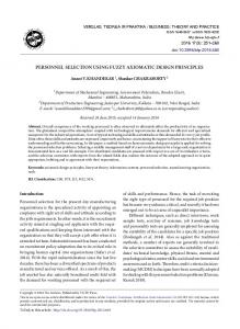
3.1 Result To identify the efficiency of the newly developed VSFI algorithm, the experimental results are compared with that of the AHP algorithm. The main goals of VSFI were to reduce the time, make it user friendly, and to reduce the implementation complexity for huge number of criteria and vendors. To examine that, it needs to put the algorithm in a highly contrary situation and hence three test cases are considered where the worst case situation contains 1000 vendors with 16 criteria. Three test cases are formed: (1) Exactly 150 vendors for sixteen selection criteria; (2) Exactly 500 vendors for sixteen selection criteria; (3) Exactly 1000 vendors for sixteen selection criteria. In the first case, with sixteen criteria and 150 vendors with their specification sheet, AHP has produced the result within 23.67 minutes. It has required 150150 matrices to solve the case and also needs 150 vendors at a time to compute the result and hence AHP has become so brute force and time consuming. On the other hand, the proposed VSFI algorithm has taken only 3.37 minutes due to working with four vendors in ranking stage and also iteratively dividing the problem set into four groups while rejecting three groups during each iteration. Hence, the VSFI algorithm is highly efficient algorithm to find out the best vendor. Another experiment with 500 vendors for the same sixteen criteria has been considered. In this second case of experiment, AHP has required 50.61 minutes where 20 judges have to work together to make pair-wise comparison and

Three test cases are formed: 1. Exactly 150 vendors for sixteen selection criteria 2. Exactly 500 vendors for sixteen selection criteria 3. Exactly 1000 vendors for sixteen selection criteria. In the first case, with sixteen criteria and 150 vendors with their specification sheet, AHP has produced the result within 23.67 minutes. It has requiredScience 150×150 to solve the case and 5(5): 376-382, 2010 International Journal of Management andmatrices Engineering Management, 381 also needs 150 vendors at a time to compute the result and hence AHP has become so brute force and time consuming. On has the needed other hand, the matrices proposed which VSFI algorithm taken the onlyanalytic 3.37 also AHP 500500 has been has so imhierarchy process (AHP). FCM initially genminutes due topractical working and with computationally four vendors in ranking stage Judges, and alsowho iteratively the expensive. have dividing erate pseudo-partitions of four groups randomly and it calproblem set into four groups while rejecting three groups500 during each iteration. Hence,culates the VSFI expressed their judgment for those vendors, could be cluster (group) centers. Ranking these four groups algorithm is highly efficient algorithm find out level the best vendor. inconsistent with an toextreme and hence AHP has be- using these cluster centers and applying AHP, three groups Another experiment 500 vendors the contrary, same sixteen criteria been 7.65 considered. come with impractical. Onforthe VSFI hashas taken can In bethis discarded by taking the largest value having the best second case ofminutes experiment, required 50.61 20 judges to workand hence the reduction process reduced the numwithAHP onlyhas three judges to minutes take thewhere decision. This have vendors together to make pair-wise also AHP has needed 500×500 matrices ber which again provescomparison superior and performance of the VSFI algorithm of has vendors by 3/4. In this way, the VSFI reduces the been so impractical expensive. Judges, expressed judgment over and the computationally AHP algorithm. The third casewho hashave been consid-theircomputational time and required space. In the VSFI algofor those 500 vendors, could be inconsistent withthis an extreme level has and hence AHP has become ered with 1000 vendors. For case, AHP required rithm, 16 criteria are used and any number of criteria can impractical. On108.76 the contrary, VSFI has taken 7.65 minutes only three judges minutes where 20 judges have towith work together to to betake usedthebased on the requirement of the business organizadecision. This again proves superior performance of the VSFI algorithm over the AHP algorithm. give subjective judgment and AHP has needed 1000 × 1000 tion and the application. The VSFI algorithm outperforms The third case matrices has been considered with 1000too vendors. this case, AHP has required that has become muchFor impractical to implethe 108.76 AHP and requires seven times less computational time. minutes where ment. 20 judges have to work togetherhas to give subjective judgment AHP has The VSFI algorithm computed only in nineand iterDueneeded to the algorithmic formulation of the VSFI algorithm, 1000×1000 matrices too much impractical to implement. Thethe VSFIthis algorithm ationsthat andhasit become has required only 15.98 minutes to take can be used in any kinds of vendor selection problem has computed final only in nine iterations and shows it has required only 15.98 minutes to the also finalin any sort of multi-criteria decision support sysdecision. This also the superior performance of takeand decision. This also the superior performance of the proposed algorithm over AHP. the shows proposed algorithm over AHP. tems as an efficient approach.

References 150

[1] Bezdek, J. (1981). Pattern recognition with fuzzy objective function algorithm. Plenum Press, New York, 1981. [2] Bayazit, O. and Karpak, B. (2005). An AHP application in vendor selection. ISAHP’05. 50 P ropos ed [3] Bayrak, M., C ¸ elebi, N., and Taskin, H. (2007). A fuzzy apModel proach method for supplier selection. Production Planning 0 and Control, 18(1):54–63. 1000 500 150 [4] Bezdek, J. (1984). FCM: The Fuzzy c-means clustering algorithm. Computer and Geosciences, 10(2-3):191–203. [5] Bhutta, K. and Huq, F. (2002). Supplier selection problem: Figure 4: Performance comparison between AHP Fig. and 4 Performance comparison between AHP and VSFI a comparison of the total cost of ownership and analytic hiVSFI erarchy process approaches. Supply Chain Management: An International Journal, 7(3):126–135. 3.2 Analysis 4.2 Analysis [6] Boer, L., der Wegen, L., and Telgen, J. (1998). Outranking 4 above proves that the VSFI algorithm reduces deciFig. Figure 4 above proves that the VSFI algorithm reduces decision making time significantly as in support of supplier selection. European Journal methods making time as compared with AHP. For compared withsion AHP. For 150, 500significantly and 1000 vendors, the VSFI algorithm reduced the time of Purchasing and Supply Management, 4(2):109–118. 150,6.59 500times, and6.74 1000 vendors, the VSFI algorithm complexity about times and 6.80 times respectively. Onreduced an average,[7] it reduces Buffa, F. and Jackson, W. (1983). A goal programming the time complexity about 6.59 times, 6.74 times and 6.80 85.30% time. For 1000 vendors, AHP needed 1000×1000 matrixes and for each criterion modeloffor purchase planning. Journal of Purchasing and Maan average, it reduces 85.30% time. sixteen criteria times it needsrespectively. 16 matrices ofOn 1000×1000 cells that are practically very difficult toterial handle Management, 19(3):27–34. vendors, AHP needed 1000 × 1000 matrixes and and also huge For space1000 in memory is needed. This also requires computational complexity into a M. and Wang, S. (1999). Fuzzy clustering analysis for [8] Chen, for each criterion of sixteen criteria it needs 16 matrices of optimizing fuzzy membership function. International Journal 1000 × 1000 cells that are practically very difficult to handle on Fuzzy sets and systems, 10(3):239–254. and also huge space in memory is needed. This also requires [9] Degraeve, Z., Roodhooft, F., and van Doveren, B. (2005). computational complexity into a massive scale. Use of FCM The use of total cost of ownership for strategic procurement: A company-wide management information system. Journal of clustering algorithm confirms that only four vendors is anthe Operational Research Society, 56(1):51–59. alyzed further in AHP. So 4 × 4 matrices are enough for the calculation. In this way, it reduces the space and computa- [10] Ellram, L. (1990). The supplier selection decision in strategic partnerships. Journal of Purchasing Materials, 26(4):8–14. tional complexity. To assess the overall performance of the VSFI algorithm, it is obvious that the time taken for AHP [11] Ghodsypour, S. and O’Brien, C. (1998). Decision support for supplier selection using an integrated Analytic Hierarchy is approximately 7 times higher than AHP as highlighted in Process and linear programming. International Journal of Fig. 4 and the reduction is significant and amazing. One of Production Economics, 56(57):199–212. the major advantages of this algorithm is that any number [12] G¨ uler, M. (2008). Incorporating multi-criteria consideraof feature or criteria can be used in FCM to classify the tions into supplier selection problem using Analytical Hiervendors according to the requirement of business organizaarchy Process: A case study. Journal of Yasar University, tion and the applications. This means the proposed VSFI 3(12):775–798. algorithm is highly accommodative and user friendly. [13] Hwang, H., Moon, C., and et al. (2005). Supplier selection and planning model using AHP. International Journal of the 4 Conclusion Information Systems for Logistics and Management, 1(1):47– 53. Among the existing vendor selection algorithms, analytic [14] Junyan, W., Ruiqing, Z., and Wansheng, T. (2008). Fuzzy hierarchy process (AHP) is able to provide a sparkling hierprogramming models for vendor selection problem in a supply archical structure (Hwang et al., 2005 [13]) and is troublechain. Tsinghua Science and Technology, 13(1):106–111. free to formulate the problem of vendor selection and hence [15] Kaur, P., Verma, R., and Mahanti, N. (2008). Vendor sewidely used to search an optimal solution. But when maslection problem using fuzzy Analytical Hierarchy Process. Insive alternatives compete to win the selection, it becomes ternational Journal of Soft Computing, 3(1):1–8. so difficult for AHP to finalize the ranking process and [16] Kubat, C. and Yuce, B. (2006). Supplier selection with gealso requires huge amount of memory space and compunetic algorithm and fuzzy AHP. In Proceedings of 5th Intertational time. Addressing these issues, this paper has pronational Symposium on Intelligent Manufacturing Systems, posed vendor selection using fuzzy integration (VSFI) algopages 1382–1401, Sakarya University, Department of Indusrithm by integrating fuzzy c-means (FCM) algorithm with trial Engineering. 100

A HP


382 [17] Millet, I. (1997). The effectiveness of Alternative Preference Elicitation Methods in the Analytic Hierarchy Process. Journal of Multi-Criteria Decision Analysis, 6(1):41–51. [18] Min, H. (1994). International supplier selection: A multiattribute utility approach. International Journal of Physical Distribution and Logistics Management, 24(5):24–33. [19] Muralidharan, C., Anantharaman, N., and Deshmukh, S. (2002). A multi-criteria group decision-making model for supplier rating. Journal of Supply Chain Management: A Global Review of Purchasing and Supply, 38(4):22–33. [20] Porter, W. (1979). How competitive forces shape strategy. Harvard Business Review. [21] Saaty, T. (1988). The Analytic Hierarchy Process. New York: McGraw-Hill. [22] Saaty, T. (1994). How to make a decision: the Analytic Hierarchy Process. Interfaces, 24(6):19–43. [23] Shil, N. (2009a). A case on vendor selection methodology: An integrated approach. Journal of Transport and Supply Chain Management, 3(1):80–95.


M. Ali & N. Shil & et al.: Vendor selection using fuzzy integration [24] Shil, N. (2009b). Management of optimum supplier selection process. Indian Management Research Journal, 1(1):4–18. [25] Ustun, O. and Demirtas, E. (2008). Multi-period lot-sizing with supplier selection using achievement scalarizing functions. Computers & Industrial Engineering, 54(4):918–931. [26] Weber, C. and Current, J. (1993). A multi-objective approach to vendor selection. European Journal of Operational Research, 68(2). [27] Wind, Y. and Robinson, P. (1968). The determinants of vendor selection: the evaluation function approach. Journal of Purchasing and Materials Management, 4(3):29–41. [28] Yigin, I., Taskin, H., and et al. (2007). Supplier selection: An expert system approach. Production Planning & Control, 18(1):16–24. [29] You, F. and Hongli, L. (2007). Information system outsourcing vendor selection based on AHP. In International Conference on Wireless Communications, Networking and Mobile Computing, pages 6250–6253.