Jan 22, 2013 - MA] 22 Jan 2013. Verification of Agent-Based Artifact Systems. Francesco Belardinelli. [email protected]. Laboratoire Ibisc, Université ...
Verification of Agent-Based Artifact Systems Francesco Belardinelli
BELARDINELLI @ IBISC . FR
Laboratoire Ibisc, Universit´e d’Evry, France
Alessio Lomuscio
A . LOMUSCIO @ IMPERIAL . AC . UK
arXiv:1301.2678v2 [cs.MA] 22 Jan 2013
Department of Computing, Imperial College London, UK
Fabio Patrizi
FABIO . PATRIZI @ DIS . UNIROMA 1. IT
Dipartimento di Ingegneria Informatica, Automatica e Gestionale “A. Ruberti” Universit`a di Roma “La Sapienza”, Italy
Abstract Artifact systems are a novel paradigm for specifying and implementing business processes described in terms of interacting modules called artifacts. Artifacts consist of data and lifecycles, accounting respectively for the relational structure of the artifacts’ states and their possible evolutions over time. In this paper we put forward artifact-centric multi-agent systems, a novel formalisation of artifact systems in the context of multi-agent systems operating on them. Differently from the usual process-based models of services, the semantics we give explicitly accounts for the data structures on which artifact systems are defined. We study the model checking problem for artifact-centric multi-agent systems against specifications written in a quantified version of temporal-epistemic logic expressing the knowledge of the agents in the exchange. We begin by noting that the problem is undecidable in general. We then identify two noteworthy restrictions, one syntactical and one semantical, that enable us to find bisimilar finite abstractions and therefore reduce the model checking problem to the instance on finite models. Under these assumptions we show that the model checking problem for these systems is EXPSPACE-complete. We then introduce artifact-centric programs, compact and declarative representations of the programs governing both the artifact system and the agents. We show that, while these in principle generate infinite-state systems, under natural conditions their verification problem can be solved on finite abstractions that can be effectively computed from the programs. Finally we exemplify the theoretical results of the paper through a mainstream procurement scenario from the artifact systems literature.
1. Introduction Much of the work in the area of reasoning about knowledge involves the development of formal techniques for the representation of epistemic properties of rational actors, or agents, in a multiagent system (MAS). The approaches based on modal logic are often rooted on interpreted systems (Parikh & Ramanujam, 1985), a computationally grounded semantics (Wooldridge, 2000) used for the interpretation of several temporal-epistemic logics. This line of research was thoroughly explored in the 1990s leading to a significant body of work (Fagin, Halpern, Moses, & Vardi, 1995). Further significant explorations have been conducted since then; a recent topic of interest has focused on the development of automatic techniques, including model checking (Clarke, Grumberg, & Peled, 1999), for the verification of temporal-epistemic specifications for the autonomous agents in a MAS (Gammie & van der Meyden, 2004; Kacprzak, Nabialek, Niewiadomski, Penczek, P´olrola, Szreter, Wozna, & Zbrzezny, 2008; Lomuscio, Qu, & Raimondi, 2009). This has led to developments in a number of areas traditionally outside artificial intelligence, knowledge representation 1
and MAS, including security (Dechesne & Wang, 2010; Ciobaca, Delaune, & Kremer, 2012), webservices (Lomuscio, Solanki, Penczek, & Szreter, 2010) and cache-coherence protocols in hardware design (Baukus & van der Meyden, 2004). The ambition of the present paper is to offer a similar change of perspective in the area of artifact systems (Cohn & Hull, 2009), a growing topic in Service-Oriented Computing (SOC). Artifacts are structures that “combine data and process in an holistic manner as the basic building block[s]” (Cohn & Hull, 2009) of systems’ descriptions. Artifact systems are services constituted by complex workflow schemes based on artifacts which the agents interact with. The data component is given by the relational databases underpinning the artifacts in a system, whereas the workflows are described by “lifecycles” associated with each artifact schema. While in the standard services paradigm services are made public by exposing their processes interface, in artifact systems both the data structures and the lifecycles are advertised. Services are composed in a “hub” where operations on the artifacts are executed. Implementations of artifact systems, such as the IBM engine BARCELONA (Heath, Hull, & Vacul´ın, 2011), provide a hub where the service choreography and service orchestratation (Alonso, Casati, Kuno, & Machiraju, 2004) are carried out. While artifact systems are beginning to drive new application areas, such as case management systems (Marin, Hull, & Vacul´ın, 2012), we identify two shortcomings in the present state-of-theart. Firstly, the artifact systems literature (Bhattacharya, Gerede, Hull, Liu, & Su, 2007; Deutsch, Hull, Patrizi, & Vianu, 2009; Hull, 2008; Nooijen, Fahland, & Dongen, 2012) focuses exclusively on the artifacts themselves. While there is obviously a need to model and implement the artifact infrastructure, importantly we also need to account for the agents implementing the services acting on the artifact system. This is of particular relevance given that artifact systems are envisaged to play a leading role in information systems. We need to be able to reason not just about the artifact states but also about what actions specific participants are allowed and not allowed to do, what knowledge they can or cannot derive in a system run, what system state they can achieve in coordination with their peers, etc. In other words, we need to move from the description of the artifact infrastructure to one that encompasses both the agents and the infrastructure. Secondly, there is a pressing demand to provide the hub with automatic choreography and orchestration capabilities. It is well-known that choreography techniques can be leveraged on automatic model checking techniques; orchestration can be recast as a synthesis problem, which, in turn, can also benefit from model checking technology. However, while model checking and its applications are relatively well-understood in the plain process-based modelling, the presence of data makes these problems much harder and virtually unexplored. Additionally, infinite domains in the underlying databases lead to infinite state-spaces and undecidability of the model checking problem. The aim of this paper is to make a concerted contribution to both problems above. Firstly, we provide a computationally grounded semantics to systems comprising the artifact infrastructure and the agents operating on it. We use this semantics to interpret a temporal-epistemic language with first-order quantifiers to reason about the evolution of the hub as well as the knowledge of the agents in the presence of evolving, structured data. We observe that the model checking problem for these structures is undecidable in general and analyse two notable decidable fragments. In this context, a contribution we make is to provide finite abstractions to infinite-state artifact systems, thereby presenting a technique for their effective verification for a class of declarative agent-based, artifact-centric programs that we here define. We evaluate this methodology by studying its compu2
tational complexity and by demonstrating its use on a well-known scenario from the artifact systems literature. 1.1 Artifact-Centric Systems Service-oriented computing is concerned with the study and development of distributed applications that can be automatically discovered and composed by means of remote interfaces. A point of distinction over more traditional distributed systems is the interoperability and connectedness of services and the shared format for both data and remote procedure calls. Two technology-independent concepts permeate the service-oriented literature: orchestration and choreography (Alonso et al., 2004; Singh & Huhns, 2005). Orchestration involves the ordering of actions of possibly different services, facilitated by a controller or orchestrator, to achieve a certain overall goal. Choreography concerns the distributed coordination of different actions through publicly observable events to achieve a certain goal. A MAS perspective (Wooldridge, 2001) is known to be particularly helpful in service-oriented computing in that it allows us to ascribe information states and private or common goals to the various services. Under this view the agents of the system implement the services and interact with one another in a shared infrastructure or environment. A key theoretical problem in SOC is to devise effective mechanisms to verify that service composition is correct according to some specification. Techniques based on model checking (Clarke et al., 1999) and synthesis (Berardi, Cheikh, Giacomo, & Patrizi, 2008) have been put forward to solve the composition and orchestration problem for services described and advertised at interface level through finite state machines (Calvanese, Giacomo, Lenzerini, Mecella, & Patrizi, 2008). More recently, attention has turned to services described by languages such as WS-BPEL (Alves et al., 2007), which provide potentially unbounded variables in the description of the service process. Again, model checking approaches have successfully been used to verify complex service compositions (Bertoli, Pistore, & Traverso, 2010; Lomuscio, Qu, & Solanki, 2012). While WS-BPEL provides a model for services with variables, the data referenced by them is non-permanent. The area of data-centric workflows (Hull, Narendra, & Nigam, 2009; Nigam & Caswell, 2003) evolved as an attempt to provide support for permanent data, typically present in the form of underlying databases. Although usually abstracted away, permanent data is of central importance to services, which typically query data sources and are driven by the answers they obtain; see, e.g., (Berardi, Calvanese, Giacomo, Hull, & Mecella, 2005). Therefore, a faithful model of a service behavior cannot, in general, disregard this component. In response to this, proposals have been made in the workflows and service communities in terms of declarative specifications of data-centric services that are advertised for automatic discovery and composition. The artifactcentric approach (Cohn & Hull, 2009) is now one of the leading emerging paradigms in the area. As described in (Hull, 2008; Hull, Damaggio, De Masellis, Fournier, Gupta, Heath, Hobson, Linehan, Maradugu, Nigam, Sukaviriya, & Vaculin, 2011) artifact-centric systems can be presented along four dimensions. Artifacts are the holders of all structured information available in the system. In a businessoriented scenario this may include purchase orders, invoices, payment records, etc. Artifacts may be created, amended, and destroyed at run time; however, abstract artifact schemas are provided at design time to define the structure of all artifacts to be manipulated in the system. Intuitively, external events cause changes in the system, including in the value of artifact attributes. 3
The evolution of artifacts is governed by lifecycles. These capture the changes that an artifact may go through from creation to deletion. Intuitively, a purchase order may be created, amended and operated on by several events before it is fullfilled and its existence in the system terminated: a lifecycle associated with a purchase order artifact formalises these transitions. Services are seen as the actors operating on the artifact system. They represent both human and software actors, possibly distributed, that generate events on the artifact system. Some services may “own” artifacts, and some artifacts may be shared by several services. However, not all artifacts, or parts of artifacts, are visible to all services. Views and windows respectively determine which parts of artifacts and which artifact instances are visible to which service. An artifact hub is a system that maintains the artifact system and processes the events generated by the services. Services generate events on the artifact system according to associations. Typically these are declarative descriptions providing the precondition and postconditions for the generation of events. These generate changes in the artifact system according to the artifact lifecycles. Since events may trigger changes in several artifacts in the system, events are processed by a well-defined semantics (Damaggio, Hull, & Vacul´ın, 2011; Hull et al., 2011) that governs the sequence of changes an artifact-system may undertake upon consumption of an event. Such a semantics, based on the use of Prerequisite-Antecedent-Consequent (PAC) rules, ensures acyclicity and full determinism in the updates on the artifact system. GSM is a declarative language that can be used to describe artifact systems. BARCELONA is an engine that can be used to run a GSM-based artifact-centric system (Heath et al., 2011). The above is a partial and incomplete description of the artifact paradigm. We refer to (Cohn & Hull, 2009; Hull, 2008; Hull et al., 2011) for more details. As it will be clear in the next section, in line with the agent-based approach to services, we will use agent-based concepts to model services. The artifact-system will be represented as an environment, constituted by evolving databases, upon which the agents operate; lifecycles and associations will be modelled by local and global transition functions. The model is intended to incorporate all artifact-related concepts including views and windows. In view of the above in this paper we address the following questions. How can we give a transition-based semantics for artifacts and agents operating on them? What syntax should we use to specify properties of the agents and the artifacts themselves? Can we verify that an artifact system satisfies certain properties? As this will be shown to be undecidable, can we find suitable fragments on which this can actually be carried out? If so, what is the resulting complexity? Lastly, can we provide declarative specifications for the agent programs so that these can be verified by model checking? Can this technique be used on mainstream scenarios from the SOC literature? This paper intends to contribute answering these questions. 1.2 Related Work As stated above, virtually all current literature on artifact-centric systems focuses on properties and implementations of the artifact-system as such. Little or no attention is given to the actors on the system, whether they are human or artificial agents. A few formal techniques have, however, been put forward to verify the core, non-agent aspects of the system; in the following we briefly compare these to this contribution. To our knowledge the verification of artifact-centric business processes was first discussed in (Bhattacharya et al., 2007), where reachability and deadlocks are phrased in the context of 4
artifact-centric systems and complexity results for the verification problem are given. The present contribution differs markedly from (Bhattacharya et al., 2007) by employing a more expressive specification language, even if the agent-related aspects are not considered, and by putting forward effective abstraction procedures for verification. In (Gerede & Su, 2007) a verification technique for artifact-centric systems against a variant of computation-tree logic is put forward. The decidability of the verification problem is proven for the language considered under the assumption that the interpretation domain is bounded. Decidability is also shown for the unbounded case by making restrictions on the values that quantified variables can range over. In the work here presented we also work on unbounded domains, but do not require the restrictions present in (Gerede & Su, 2007): we only insist on the fact that the number of distinct values in the system does not exceed a given threshold at any point in any run. Most importantly, the interplay between quantification and modalities here considered allows us to bind and use variables in different states. This is a major difference as this feature is very expressive and known to lead to undecidability. A related line of research is followed in (Deutsch et al., 2009; Damaggio, Deutsch, & Vianu, 2012), where the verification problem for artifact systems against two variants of first-order lineartime temporal logic is considered. Decidability of the verification problem is retained by imposing syntactic restrictions on both the system descriptions and the specifications to check. This effectively limits the way in which new values introduced at every computational step can be used by the system. Properties based on arithmetic operators are considered in (Damaggio et al., 2012). While there are elements of similarity between these approaches and the one we put forward here, including the fact that the concrete interpretation domain is replaced by an abstract one, the contribution here presented has significant differences from these. Firstly, our setting is branching-time and not linear-time thereby resulting in different expressive power. Secondly, differently from (Deutsch et al., 2009; Damaggio et al., 2012), we impose no constraints on nested quantifiers. In contrast, (Damaggio et al., 2012) admits only universal quantification over combinations of quantifier-free first-order formulas. Thirdly, the abstraction results we present here are given in general terms on the semantics of declarative programs and do not depend on a particular presentation of the system. More closely related to the present contribution is (Hariri, Calvanese, Giacomo, Deutsch, & Montali, 2012), where conditions for the decidability of the model checking problem for datacentric dynamic systems, e.g., dynamic systems with relational states, are given. In this case the specification language used is a first-order version of the µ-calculus. While our temporal fragment is subsumed by the µ-calculus, since we use indexed epistemic modalities as well as a common knowledge operator, the two specification languages have different expressive power. To retain decidability, like we do here, the authors assume a constraint on the size of the states. However, differently from the contribution here presented, (Hariri et al., 2012) assume limited forms of quantification whereby only individuals persisting in the system evolution can be quantified over. In this contribution we do not make this restriction. Irrespective of what above, the most important feature that characterises our work is that the set-up is entirely based on epistemic logic and multi-agent systems. We use agents to represent the autonomous services operating in the system and agent-based concepts play a key role in the modelling, the specifications, and the verification techniques put forward. Differently from all approaches presented above we are not only concerned with whether the artifact-system meets a particular specification. Instead, we also wish to consider what knowledge the agents in the system acquire by interacting among themselves and with the artifact-system during a system run. Ad5
ditionally, the abstraction methodology put forward is modular with respect to the agents in the system. These features enable us to give constructive procedures for the generation of finite abstractions for artifact-centric programs associated with infinite models. We are not aware of any work in the literature tackling any of these aspects. Relation to previous work by the authors. This paper combines and expands preliminary results originally discussed in (Belardinelli, Lomuscio, & Patrizi, 2011a), (Belardinelli, Lomuscio, & Patrizi, 2011b), (Belardinelli, Lomuscio, & Patrizi, 2012a), and (Belardinelli, Lomuscio, & Patrizi, 2012b). In particular, the technical set up of artifacts and agents is different from that of our preliminary studies and makes it more natural to express artifact-centric concepts such as views. Differently from our previous attempts we here incorporate an operator for common knowledge and provide constructive methods to define abstractions for all notions of bisimulation. We also consider the complexity of the verification problem, previously unexplored, and evaluate the technique in detail on a case study. 1.3 Scheme of the Paper The rest of the paper is organised as follows. In Section 2 we introduce Artifact-centric MultiAgent Systems (ACMAS), the semantics we will be using throughout the paper to describe agents operating on an artifact system. In the same section we put forward FO-CTLK, a first-order logic with knowledge and time to reason about the evolution of the knowledge of the agents and the artifact system. This enables us to propose a satisfaction relation based on the notion of bounded quantification, define the model checking problem, and highlight some properties of isomorphic states. An immediate result we will explore concerns the undecidability of the model checking problem for ACMAS in their general setting. Section 3 is concerned with synctactical restrictions on FOCTLK that enable us to guarantee the existence of finite abstractions of infinite-state ACMAS, thereby making the model checking problem feasible by means of standard techniques. Section 4 tackles restrictions orthogonal to those of Section 3 by focusing on a subclass of ACMAS that admits a decidable model checking problem when considering full FO-CTLK specifications. The key finding here is that bounded and uniform ACMAS, a class identified by studying a strong bisimulation relation, admit finite abstractions for any FO-CTLK specification. The section concludes by showing that under these restrictions the model checking problem is EXPSPACEcomplete. We turn our attention to artifact programs in Section 6 by defining the concept of artifact-centric programs. We define them through natural, first-order preconditions and postconditions in line with the artifact-centric approach. We give a semantics to them in terms of ACMAS and show that their generated models are precisely those uniform ACMAS studied earlier in the paper. It follows that, under some boundedness conditions, which can be naturally expressed, the model checking problem for artifact-centric programs is decidable and can be executed on finite models. Section 7 reports a scenario from the artifact systems literature. This is used to exemplify the technique by providing finite abstractions that can be effectively verified. We conclude in Section 8 where we consider the limitations of the approach and point to further work. 6
2. Artifact-Centric Multi-Agent Systems In this section we formalise artifact-centric systems and state their verification problem. As data and databases are important constituents of artifact systems, our formalisation of artifacts relies on them as underpinning concepts. However, as discussed in the previous section, we here give prominence to agent-based concepts. As such, we define our systems as comprising both the artifacts in the system as well as the agents that interact with the system. A standard paradigm for logic-based reasoning about agent systems is interpreted systems (Parikh & Ramanujam, 1985; Fagin et al., 1995). In this setting agents are endowed with private local states and evolve by performing actions according to an individual protocol. As data play a key part, as well as to allow us to specify properties of the artifact system, we will define the agents’ local states as evolving database instances. We call this formalisation artifact-centric multi-agent systems (ACMAS). AC-MAS enable us to represent naturally and concisely concepts much used in the artifact paradigm such as the one of view discussed earlier. Our specification language will include temporal-epistemic logic but also quantification over a domain so as to represent the data. This is an usual verification setting, so we will formally define the model checking problem for this set up. 2.1 Databases and First-Order Logic As discussed above, we use databases as the basic building blocks for defining the states of the agents and the artifact system. We here fix the notation and terminology used. We refer to (Abiteboul, Hull, & Vianu, 1995) for more details on databases. Definition 2.1 (Database Schemas) A (relational) database schema is a set D = {P1 /q1 , . . . , Pn /qn } of relation symbols Pi , each associated with its arity qi ∈ N. Instances of database schemas are defined over interpretation domains. Definition 2.2 (Database Instances) Given an interpretation domain U and a database schema D, a D-instance over U is a mapping D associating each relation symbol Pi ∈ D with a finite qi -ary relation over U , i.e., D(Pi ) ⊆ U qi . The set of all D-instances over an interpretation domain U is denoted by D(U ). We simply refer to “instances” whenever the database schema D is clear by the context. The active domain of an instance D, denoted as adom(D), is the set of all individuals in U occurring in some tuple of some predicate interpretation D(Pi ). Observe that, since D contains a finite number of relation symbols and each D(Pi ) is finite, so is adom(D). To fix the notation, we recall the syntax of first-order formulas with equality and no function symbols. Let V ar be a countable set of individual variables and C be a finite set of individual constants. A term is any element t ∈ V ar ∪ C. Definition 2.3 (FO-formulas over D) Given a database schema D, the formulas ϕ of the firstorder language LD are defined by the following BNF grammar: ϕ ::= t = t′ | Pi (t1 , . . . , tqi ) | ¬ϕ | ϕ → ϕ | ∀xϕ where Pi ∈ D, t1 , . . . , tqi is a qi -tuple of terms and t, t′ are terms. 7
We assume “=” to be a special binary predicate with fixed obvious interpretation. To summarise, LD is a first-order language with equality over the relational vocabulary D with no function symbols and with finitely many constant symbols from C. Observe that considering a finite set of constants is not a limitation. Indeed, since we will be working with finite sets of formulas, C can always be defined so as to be able to express any formula of interest. In the following we use the standard abbreviations ∃, ∧, ∨, and 6=. Also, free and bound variables are defined as standard. For a formula ϕ we denote the set of its variables as vars(ϕ), the set of its free variables as free(ϕ), and the set of its constants as const(ϕ). We write ϕ(~x) to list explicitly in arbitrary order all the free variables x1 , . . . , xℓ of ϕ. By slight abuse of notation, we treat ~x as a set, thus we write ~x = free(ϕ). A sentence is a formula with no free variables. Given an interpretation domain U such� that C ⊆ U , an assignment is a function σ : V ar 7→ U . � For �an assignment σ, we denote by σ ux the assignment such that: (i) σ xu (x) = u; and (ii) σ xu (x′ ) = σ(x′ ), for every x′ ∈ V ar different from x. For convenience, we extend assignments to constants so that σ(t) = t, if t ∈ C; that is, we assume a Herbrand interpretation of constants. We can now define the semantics of LD . Definition 2.4 (Satisfaction of FO-formulas) Given a D-instance D, an assignment σ, and an FO-formula ϕ ∈ LD , we inductively define whether D satisfies ϕ under σ, written (D, σ) |= ϕ, as follows: (D, σ) |= Pi (t1 , . . . , tqi ) (D, σ) |= t = t′ (D, σ) |= ¬ϕ (D, σ) |= ϕ → ψ (D, σ) |= ∀xϕ
iff iff iff iff iff
hσ(t1 ), . . . , σ(tqi )i ∈ D(Pi ) σ(t) = σ(t′ ) it is not the case that (D, σ) |= ϕ (D, σ) |= ¬ϕ or (D, σ) |= ψ � for all u ∈ adom(D), we have that (D, σ ux ) |= ϕ
A formula ϕ is true in D, written D |= ϕ, iff (D, σ) |= ϕ, for all assignments σ.
Observe that we adopt an active-domain semantics, that is, quantified variables range only over the active domain of D. Also notice that constants are interpreted rigidly; so, two constants are equal if and only if they are syntactically the same. In the rest of the paper, we assume that every interpretation domain includes C. Also, as a usual shortcut, we write (D, σ) 6|= ϕ to express that it is not the case that (D, σ) |= ϕ. Finally, we introduce the ⊕ operator on D-instances that will be used later in the paper. Let the primed version of a database schema D be the schema D ′ = {P1′ /q1 , . . . , Pn′ /qn } obtained from D by syntactically replacing each predicate symbol Pi with its primed version Pi′ of the same arity. Definition 2.5 (⊕ Operator) Given two D-instances D and D ′ , we define D ⊕ D ′ as the (D ∪ D ′ )instance such that D ⊕ D ′ (Pi ) = D(Pi ) and D ⊕ D ′ (Pi′ ) = D ′ (Pi ). Intuitively, the ⊕ operator defines a disjunctive join of the two instances, where relation symbols in D are interpreted according to D, while their primed versions are interpreted according to D ′ . 2.2 Artifact-Centric Multi-Agent Systems In the following we introduce the semantic structures that we will use throughout the paper. We define an artifact-centric multi-agent system as a system comprising an environment representing all interacting artifacts in the system and a finite set of agents interacting with such environment. 8
As agents have views of the artifact state, i.e., projections of the status of particular artifacts, we assume the building blocks of their private local states also to be modelled as database instances. In line with the interpreted systems semantics (Fagin et al., 1995) not everything in the agents’ states needs to be present in the environment; a portion of it may be entirely private and not replicated in other agents’ states. So, we start by introducing the notion of agent. Definition 2.6 (Agent) Given an interpretation domain U , an agent is a tuple A = hD, L, Act, P ri, where: • D is the local database schema; • L ⊆ D(U ) is the set of local states; • Act is the finite set of action types of the form α(~ p), where p~ is the tuple of abstract parameters; • P r : L 7→ 2Act(U ) is the local protocol function, where Act(U ) is the set of ground actions of the form α(~u) where α(~ p) ∈ Act and ~u ∈ U |~p| is a tuple of ground parameters. Intuitively, at a given time each agent A is in some local state l ∈ D(U ) that represents all the information agent A has at its disposal. In this sense we follow (Fagin et al., 1995) but require that this information is structured as a database. Again, following standard literature we assume that the agents are autonomous and proactive and perform the actions in Act according to the protocol function P r. In the definition above we distinguish between “abstract parameters” to denote the language in which particular action parameters are given, and their concrete values or “ground parameters”. We assume that the agents interact among themselves and with an environment comprising all artifacts in the system. As artifacts are entities involving both data and process, we can see them as collections of database instances paired with actions and governed by special protocols. Without loss of generality we can assume the environment state to be a single database instance including all artifacts in the system. From a purely formal point of view this allows us to represent the environment as a special agent. Of course, in any specific instantiation the environment and the agents will be rather different, exactly in line with the standard propositional version of interpreted systems. We can therefore define the synchronous composition of agents with the environment. Definition 2.7 (Artifact-Centric Multi-Agent Systems) Given an interpretation domain U and a set Ag = {A0 , . . . , An } of agents Ai = hDi , Li , Acti , P ri i defined on U , an artifact-centric multiagent system (or AC-MAS) is a tuple P = hS, U, s0 , τ i where: • S ⊆ L0 × · · · × Ln is the set of reachable global states; • U is the interpretation domain; • s0 ∈ S is the initial global state; • τ : S × Act(U ) 7→ 2S is the global transition function, where Act(U ) = Act0 (U ) × · · · × Actn (U ) is the set of global (ground) actions, and τ (hl0 , . . . , ln i, hα0 (~u0 ), . . . , αn (~un )i) is defined iff αi (~ui ) ∈ P ri (li ) for every i ≤ n. 9
As we will see in later sections, AC-MAS are the natural extension of interpreted systems to the first order to account for environments constituted of artifact-centric systems. They can be seen as a specialisation of quantified interpreted systems (Belardinelli & Lomuscio, 2012), a general extension of interpreted systems to the first-order case. In the formalisation above the agent A0 is referred to as the environment E. The environment includes all artifacts in the system as well as additional information to facilitate communication between the agents and the hub, e.g., messages in transit etc. At any given time an AC-MAS is described by a tuple of database instances, representing all the agents in the system as well as the artifact system. A single interpretation domain for all database schemas is given. Note that this does not break the generality of the representation as we can always extend the domain of all agents and the environment before composing them into a single AC-MAS. The global transition function defines the evolution of the system through synchronous composition of actions for the environment and all agents in the system. Much of the interaction we are interested in modelling involves message exchanges with payload, hence the action parameters, between agents and the environment, i.e., agents operating on the artifacts. However, note that the formalisation above does not preclude us from modelling agent-toagent interactions, as the global transition function does not rule out successors in which only some agents change their local state following some actions. Also observe that essential concepts such as views are naturally expressed in AC-MAS by insisting that the local state of an agent includes part of the environment’s, i.e., the artifacts the agent has access to. Not all AC-MAS need to have views defined, so it is also possible for the views to be empty. Other artifact-based concepts such as lifecycles are naturally expressed in AC-MAS. As artifacts are modelled as part of the environment, a lifecycle is naturally encoded in AC-MAS simply as the sequence of changes induced by the transition function τ on the fragment of the environment representing the lifecycle in question. We will show an example of this in Section 7. Some technical remarks now follow. To simplify the notation, we denote a global ground action as α ~ (~u), where α ~ = hα0 (p0 ), . . . , αn (pn )i and ~u = h~u0 , . . . , ~un i, with each ~ui of appropriate size. We define the transition relation → on S × S such that s → s′ if and only if there exists a α ~ (~u) ∈ Act(U ) such that s′ ∈ τ (s, α ~ (~u)). If s → s′ , we say that s′ is a successor of s. A run r . 0 from s ∈ S is an infinite sequence s → s1 → · · · , with s0 = s. For n ∈ N, we take r(n) = sn . A state s′ is reachable from s if there exists a run r from the global state r(0) = s such that r(i) = s′ , for some i ≥ 0. We assume that the relation → is serial. This can be easily obtained by assuming that each agent has a skip action enabled at each local state and that performing skip induces no changes in any of the local states. We consider S to be the set of states reachable from the initial state s0 . For convenience we will use also the concept of temporal-epistemic (t.e., for short) run. Formally a t.e. run r from a state s ∈ S is an infinite sequence s0 ❀ s1 ❀ . . . such that s0 = s and si → si+1 or si ∼k si+1 , for some k ∈ Ag. A state s′ is said to be temporally-epistemically reachable (t.e. reachable, for short) from s if there exists a t.e. run r from the global state r(0) = s such that for some i ≥ 0 we have that r(i) = s′ . Obviously, temporal-epistemic runs include purely temporal runs as a special case. As in plain interpreted systems (Fagin et al., 1995), we say that two global states s = hl0 , . . . , ln i and s′ = hl0′ , . . . , ln′ i are epistemically indistinguishable for agent Ai , written s ∼i s′ , if li = li′ . Differently from interpreted systems the local equality is evaluated on database instances. Also, notice that we admit U to be infinite, thereby allowing the possibility of the set of states S to be 10
infinite. Indeed, unless we specify otherwise, we will assume to be working with infinite-state AC-MAS. Finally, for technical reasons it is useful to refer to a global database schema D = D0 ∪ · · · ∪ Dn of an AC-MAS. Every global state S s = hl0 , . . . , ln i is associated with the (global) D-instance Ds ∈ D(U ) such that Ds (Pi ) = j∈Ag lj (Pi ), for Pi ∈ D. We omit the subscript s when s is clear from the context and we write adom(s) for adom(Ds ). Notice that for every s ∈ S, the Ds associated with s is unique, while the converse is not true in general. 2.3 Model Checking We now define the problem of verifying an artifact-centric multi-agent system against a specification of interest. By following the artifact-centric model, we wish to give data the same prominence as processes. To deal with data and the underlying database instances, our specification language needs to include first-order logic. Further, we require temporal logic to describe the system execution. Lastly, we use epistemic logic to express the information the agents have at their disposal. Hence, we define a first-order temporal epistemic specification language to be interpreted on AC-MAS. The specification language will be used in Section 6 to formalise properties of artifact-centric programs. Definition 2.8 (The Logic FO-CTLK) The first-order CTLK (or FO-CTLK) formulas ϕ over a database schema D are inductively defined by the following BNF: ϕ ::= φ | ¬ϕ | ϕ → ϕ | ∀xϕ | AXϕ | AϕU ϕ | EϕU ϕ | Ki ϕ | Cϕ where φ ∈ LD and 0 < i ≤ n. The notions of free and bound variables for FO-CTLK extend straightforwardly from LD , as well as functions vars, free, and const. As usual, the temporal formulas AXϕ and AϕU ϕ′ (resp. EϕU ϕ′ ) are read as “for all runs, at the next step ϕ” and “for all runs (resp. some run), ϕ until ϕ′ ”. The epistemic formulas Ki ϕ and Cϕ intuitively mean that “agent Ai knows ϕ” and “it is common knowledge among all agents that ϕ” respectively. We use the abbreviations EXϕ, AF ϕ, AGϕ, EF ϕ, and EGϕ as standard. Observe that free variables can occur within the scope of modal operators, thus allowing for the unconstrained alternation of quantifiers and modal operators, thereby allowing us to refer to elements in different modal contexts. We consider also a number of fragments of FO-CTLK. The sentence atomic version of FO-CTLK without epistemic modalities, or SA-FO-CTL, is the language obtained from Definition 2.8 by removing the clauses for epistemic operators and restricting atomic formulas to first-order sentences, so that no variable appears free in the scope of a modal operator: ϕ ::= φ | ¬ϕ | ϕ → ϕ | AXϕ | AϕU ϕ | EϕU ϕ where φ ∈ LD is a sentence. We will consider also the language FO-ECTLK, i.e., the existential fragments of FO-CTLK, defined as follows: ¯ i ϕ | Cϕ, ¯ ϕ ::= φ | ϕ ∧ ϕ | ϕ ∨ ϕ | ∀xϕ | ∃xϕ | EXϕ | EϕU ϕ | K ¯ i ϕ ≡ ¬Ki ¬ϕ, and Cϕ ¯ ≡ ¬C¬ϕ. where φ ∈ LD , with ∧ and ∨ the standard abbreviations, K The semantics of FO-CTLK formulas is defined as follows. 11
Definition 2.9 (Satisfaction for FO-CTLK) Consider an AC-MAS P, an FO-CTLK formula ϕ, a state s ∈ P, and an assignment σ. We inductively define whether P satisfies ϕ in s under σ, written (P, s, σ) |= ϕ, as follows: (P, s, σ) |= ϕ (P, s, σ) |= ¬ϕ (P, s, σ) |= ϕ → ϕ′ (P, s, σ) |= ∀xϕ (P, s, σ) |= AXϕ (P, s, σ) |= AϕU ϕ′
(Ds , σ) |= ϕ, if ϕ is an FO-formula it is not the case that (P, s, σ) |= ϕ (P, s, σ) |= ¬ϕ or (P, s, σ) |= �ϕ′ for all u ∈ adom(s), (P, s, σ xu ) |= ϕ for all runs r, if r(0) = s, then (P, r(1), σ) |= ϕ for all runs r, if r(0) = s, then there is k ≥ 0 s.t. (P, r(k), σ) |= ϕ′ , and for all j, 0 ≤ j < k implies (P, r(j), σ) |= ϕ (P, s, σ) |= EϕU ϕ′ iff for some run r, r(0) = s and there is k ≥ 0 s.t. (P, r(k), σ) |= ϕ′ , and for all j, 0 ≤ j < k implies (P, r(j), σ) |= ϕ (P, s, σ) |= Ki ϕ iff for all s′ , s ∼i s′ implies (P, s′ , σ) |= ϕ (P, s, σ) |= Cϕ iff for all s′ , s ∼ s′ implies (P, s′ , σ) |= ϕ S where ∼ is the transitive closure of 1...n ∼i . iff iff iff iff iff iff
A formula ϕ is said to be true at a state s, written (P, s) |= ϕ, if (P, s, σ) |= ϕ for all assignments σ. Moreover, ϕ is said to be true in P, written P |= ϕ, if (P, s0 ) |= ϕ. A key concern in this paper is to explore the model checking of AC-MAS against first-order temporal-epistemic specifications.
Definition 2.10 (Model Checking) Model checking an AC-MAS P against an FO-CTLK formula ϕ amounts to finding an assignment σ such that (P, s0 , σ) |= ϕ. It is easy to see that whenever U is finite the model checking problem is decidable as P is a finitestate system. In general this is not the case. Theorem 2.11 The model checking problem for AC-MAS w.r.t. FO-CTLK is undecidable. Proof (sketch). This can be proved by showing that every Turing machine T whose tape contains an initial input I can be simulated by an artifact system PT,I . The problem of checking whether T terminates on that particular input can be reduced to checking whether PT,I |= ϕ, where ϕ encodes the termination condition. The detailed construction is similar to that of Theorem 4.10 of (Deutsch, Sui, & Vianu, 2007). Given the general setting in which the model checking problem is defined above, the negative result is not surprising. In the following we identify syntactic and semantic restrictions for which the problem is decidable. 2.4 Isomorphisms We now investigate the concept of isomorphism on AC-MAS. This will be needed in later sections to produce finite abstractions of infinite-state AC-MAS. In what follows let P = hS, U, s0 , τ i and P ′ = hS ′ , U ′ , s′0 , τ i be two AC-MAS. Definition 2.12 (Isomorphism) Two local states l, l′ ∈ D(U ) are isomorphic, written l ≃ l′ , iff there exists a bijection ι : adom(l) ∪ C 7→ adom(l′ ) ∪ C such that: 12
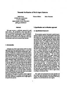
l(P1 ) a b b d
l(P2 ) a
l′ (P1 ) c b b e
l′ (P2 ) c
l′′ (P1 ) f d d e
l′′ (P2 ) f
Figure 1: Examples of isomorphic and non-isomorphic local states. (i) ι is the identity on C; (ii) for every Pi ∈ D, ~u ∈ U qi , we have that ~u ∈ l(Pi ) iff ι(~u) ∈ l′ (Pi ). When this is the case, we say that ι is a witness for l ≃ l′ . Two global states s ∈ S and s′ ∈ S ′ are isomorphic, written s ≃ s′ , iff there exists a bijection ι : adom(s) ∪ C 7→ adom(s′ ) ∪ C such that for every j ∈ Ag, ι is a witness for lj ≃ lj′ . Notice that isomorphisms preserve the constants in C as well as predicates in the local states up to renaming of the corresponding terms. Any function ι as above is called a witness for s ≃ s′ . Obviously, the relation ≃ is an equivalence relation. Given a function f : U 7→ U ′ defined on adom(s), f (s) denotes the interpretation in D(U ′ ) obtained from s by renaming each u ∈ adom(s) as f (u). If f is also injective (thus invertible) and the identity on C, then f (s) ≃ s. Example. For an example of isomorphic states, consider an agent with local database schema D = {P1 /2, P2 /1}, let U = {a, b, c, . . .} be an interpretation domain, and fix the set C = {b} of constants. Let l be the local state such that l(P1 ) = {ha, bi, hb, di} and l(P2 ) = {a} (see Figure 1). Then, the local state l′ such that l′ (P1 ) = {hc, bi, hb, ei} and l′ (P2 ) = {c} is isomorphic to l. This can be easily seen by considering the isomorphism ι, where: ι(a) = c, ι(b) = b, and ι(d) = e. On the other hand, the state l′′ where l′′ (P1 ) = {hf, di, hd, ei} and l′′ (P2 ) = {f } is not isomorphic to l. Indeed, although a bijection exists that “transforms” l into l′′ , it is easy to see that none can be such that ι′ (b) = b. Note that, while isomorphic states have the same relational structure, two isomorphic states do not necessarily satisfy the same FO-formulas as satisfaction depends also on the values assigned to free variables. To account for this, we introduce the following notion. Definition 2.13 (Equivalent assignments) Given two states s ∈ S and s′ ∈ S ′ , and a set of variables V ⊆ V ar, two assignments σ : V ar 7→ U and σ ′ : V ar 7→ U ′ are equivalent for V w.r.t. s and s′ iff there exists a bijection γ : adom(s) ∪ C ∪ σ(V ) 7→ adom(s′ ) ∪ C ∪ σ ′ (V ) such that: (i) γ|adom(s)∪C is a witness for s ≃ s′ ; (ii) σ ′ |V = γ ◦ σ|V . Intuitively, equivalent assignments preserve both the (in)equalities of the variables in V and the constants in s, s′ up to renaming. Note that, by definition, the above implies that s, s′ are isomorphic. We say that two assignments are equivalent for an FO-CTLK formula ϕ, omitting the states s and s′ when it is clear from the context, if these are equivalent for free(ϕ). We can now show that isomorphic states satisfy exactly the same FO-formulas. Proposition 2.14 Given two isomorphic states s ∈ S and s′ ∈ S ′ , an FO-formula ϕ, and two assignments σ and σ ′ equivalent for ϕ, we have that (Ds , σ) |= ϕ iff (Ds′ , σ ′ ) |= ϕ 13
Proof. The proof is by induction on the structure of ϕ. Consider the base case for the atomic formula ϕ ≡ P (t1 , . . . , tk ). Then (Ds , σ) |= ϕ iff hσ(t1 ), . . . , σ(tk )i ∈ Ds (P ). Since σ and σ ′ are equivalent for ϕ, and s ≃ s′ , this is the case iff hσ ′ (t1 ), . . . , σ ′ (tk )i ∈ Ds′ (P ), that is, (Ds′ , σ ′ ) |= ϕ. The base case for ϕ ≡ t = t′ is proved similarly, by observing that the satisfaction of ϕ depends only on the assignments, and that the function γ of Def. 2.13 is a bijection, thus all the (in)equalities between the values assigned by σ and σ ′ are preserved. This is sufficient to guarantee that σ(t) = σ(t′ ) iff σ ′ (t) = σ ′ (t′ ). The inductive step for the propositional connectives � is straightforward. Finally, if ϕ ≡ ∀yψ, then (Ds , σ) |= ϕ iff for all u ∈ adom(s), (Ds , σ uy ) |= ψ.� Now consider the witness ι = γ|adom(s)∪C for s ≃ s′ , where γ is as in Def. 2.13. We have that σ uy y � y � y� ′ ′ and σ ι(u) are equivalent for ψ. By induction hypothesis (Ds , σ u ) |= ψ iff (Ds′ , σ ι(u) ) |= ψ. � Since ι is a bijection, this is the case iff for all u′ ∈ adom(s′ ), (Ds′ , σ ′ uy′ ) |= ψ, i.e., (Ds′ , σ ′ ) |= ϕ. This leads us to the following result. Corollary 2.15 Given two isomorphic states s ∈ S and s′ ∈ S ′ and an FO-sentence ϕ, we have that Ds |= ϕ iff Ds′ |= ϕ Proof. From right to left. Suppose, by contradiction, that Ds 6|= ϕ. Then there exists an assignment σ s.t. (Ds , σ) 6|= ϕ. Since free(ϕ) = ∅, if ι is a witness for s ≃ s′ , then the assignment σ ′ = ι ◦ σ is equivalent to σ for s and s′ . By Proposition 2.14 we have that (Ds′ , σ ′ ) 6|= ϕ, that is, Ds′ 6|= ϕ. The case from left to right can be shown similarly. Thus, isomorphic states cannot be distinguished by FO-sentences. This enables us to use this notion when defining simulations as we will see in the next section.
3. Abstractions for Sentence Atomic FO-CTL In the previous section we have observed that model checking AC-MAS against FO-CTLK is undecidable in general. So, it is clearly of interest to identify decidable settings. In what follows we introduce two main results. The first, presented in this section, identifies restrictions on the language; the second, presented in the next section, focuses on semantic constraints. While these cases are in some sense orthogonal to each other, we show that they both lead to decidable model checking problems. They are also both carried out on a rather natural subclass of AC-MAS that we call bounded, which we identify below. Our goal for proceeding in this manner is to identify finite abstractions of infinite-state AC-MAS so that verification of programs, that admit AC-MAS as models, can be conducted on them, rather than on infinite-state AC-MAS. We will see this in detail in Section 6. Given our aims we begin by defining a first notion of bisimulation in the context of AC-MAS. Bisimulations will be used to show that all bounded AC-MAS admit a finite, bisimilar, abstraction that satisifies the same SA-FO-CTL specifications as the original AC-MAS. Also in what follows we assume that P = hS, U, s0 , τ i and P ′ = hS ′ , U ′ , s′0 , τ ′ i. Definition 3.1 (Simulation) A relation R ⊆ S × S ′ is a simulation iff hs, s′ i ∈ R implies: 1. s ≃ s′ ; 14
2. for every t ∈ S, if s → t then there exists t′ ∈ S ′ s.t. s′ → t′ and ht, t′ i ∈ R. Definition 3.1 presents the standard notion of simulation applied to the case of AC-MAS. The difference from the propositional case is that we here insist on the states being isomorphic, a generalisation from the usual requirement for propositional valuations to be equal (Blackburn, de Rijke, & Venema, 2001). As in the standard case, two states s ∈ S and s′ ∈ S ′ are said to be similar, written s � s′ , if there exists a simulation relation R s.t. hs, s′ i ∈ R. It can be proven that the similarity relation � is a simulation itself, and in particular the largest one w.r.t. set inclusion, and that it is transitive and reflexive. Finally, we say that P ′ simulates P, written P � P ′ , if s0 � s′0 . We extend the above to bisimulations. Definition 3.2 (Bisimulation) A relation B ⊆ S × S ′ is a bisimulation iff both B and B −1 = {hs′ , si | hs, s′ i ∈ B} are simulations. We say that two states s ∈ S and s′ ∈ S ′ are bisimilar, written s ≈ s′ , if there exists a bisimulation B s.t. hs, s′ i ∈ B. Similarly to simulations, it can be proven that the bisimilarity relation ≈ is the largest bismulation. Further, it is an equivalence relation. Finally, P and P ′ are said to be bisimilar, written P ≈ P ′ , if s0 ≈ s′0 . Since, as shown in Proposition 2.15, the satisfaction of FO-sentences is invariant under isomorphisms, we can now extend the usual bisimulation result from the propositional case to that of SA-FO-CTL. We begin by showing a result on bisimilar runs. Proposition 3.3 Consider two AC-MAS P and P ′ such that P ≈ P ′ , s ≈ s′ , for some s ∈ S, s′ ∈ S ′ , and a run r of P such that r(0) = s. Then there exists a run r ′ of P ′ such that: (i) r ′ (0) = s′ ; (ii) for all i ≥ 0, r(i) ≈ r ′ (i). Proof. We show by induction that such run r ′ in P ′ exists. For i = 0, let r ′ (0) = s′ . Obviously, r(0) ≈ r ′ (0). Now, assume, by induction hypothesis, that r(i) ≈ r ′ (i). Let r(i) → r(i + 1). Since r(i) ≈ r ′ (i), by Def. 3.1, there exists t′ ∈ S ′ such that r ′ (i) → t′ and r(i + 1) ≈ t′ . Let r ′ (i + 1) = t′ ; hence we obtain r(i + 1) ≈ r ′ (i + 1). By definition r ′ is a run of P ′ . This enables us to show that bisimilar AC-MAS preserve SA-FO-CTL formulas. This is an extension of analogous results on propositional CTL. Lemma 3.4 Consider the AC-MAS P and P ′ such that P ≈ P ′ , s ≈ s′ , for some s ∈ S, s′ ∈ S ′ and an SA-FO-CTL formula ϕ. Then, (P, s) |= ϕ iff (P ′ , s′ ) |= ϕ Proof. The proof is by induction on the structure of ϕ. Observe first that since ϕ is sentenceatomic, its satisfaction does not depend on assignments. We report the proof for the left-to-right part of the implication; the converse can be shown similarly. The base case for an FO-sentence ϕ follows from Prop. 2.15. The inductive cases for propositional connectives are straightforward. 15
For ϕ ≡ AXψ, assume for contradiction that (P, s) |= ϕ and (P ′ , s′ ) 6|= ϕ. Then, there exists a run r ′ s.t. r ′ (0) = s′ and (P ′ , r ′ (1)) 6|= ψ. By Def. 3.2 and 3.1 there exists a t ∈ S s.t. s → t and t ≈ r ′ (1). Further, by seriality of →, s → t can be extended to a run r s.t. r(0) = s and r(1) = t. By the induction hypothesis we obtain that (P, r(1)) 6|= ψ. Hence, (P, r(0)) 6|= AXψ, which is a contradiction. For ϕ ≡ EψU φ, let r be a run with r(0) = s such that there exists k ≥ 0 such that (P, r(k)) |= φ, and for every j, 0 ≤ j < k implies (P, r(j)) |= ψ. By Prop. 3.3 there exists a run r ′ s.t. r ′ (0) = s′ and for all i ≥ 0, r ′ (i) ≈ r(i). By the induction hypothesis we have that for each i ∈ N, (P, r(i)) |= ψ iff (P ′ , r ′ (i)) |= ψ, and (P, r(i)) |= φ iff (P ′ , r ′ (i)) |= φ. Therefore, r ′ is a run s.t. r ′ (0) = s′ , (P ′ , r ′ (k)) |= φ, and for every j, 0 ≤ j < k implies (P ′ , r ′ (j)) |= ψ, i.e., (P ′ , s′ ) |= EψU φ. For ϕ ≡ AψU φ, assume for contradiction that (P, s) |= ϕ and (P ′ , s′ ) 6|= ϕ. Then, there exists a run r ′ s.t. r ′ (0) = s′ and for every k ≥ 0, if (P ′ , r ′ (k)) |= φ, then there exists j s.t. 0 ≤ j < k and (P ′ , r ′ (j)) 6|= ψ. By Prop. 3.3 there exists a run r s.t. r(0) = s and for all i ≥ 0, r(i) ≈ r ′ (i). Further, by the induction hypothesis we have that (P, r(i)) |= ψ iff (P ′ , r ′ (i)) |= ψ and (P, r(i)) |= φ iff (P ′ , r ′ (i)) |= φ. But then r is s.t. r(0) = s and for every k ≥ 0, if (P, r(k)) |= φ, then there exists j s.t. 0 ≤ j < k and (P, r(j)) 6|= ψ. That is, (P, s) 6|= AψU φ, which is a contradiction. By applying the result above to the case of s = s0 and s′ = s′0 , we obtain the following. Theorem 3.5 Consider the AC-MAS P and P ′ such that P ≈ P ′ , and an SA-FO-CTL formula ϕ. We have P |= ϕ iff P ′ |= ϕ In summary we have proved that bisimilar AC-MAS validate the same SA-FO-CTL formulas. In the next section we use this result to reduce, under additional assumptions, the verification of an infinite-state AC-MAS to that of a finite-state one. 3.1 Finite Abstractions of Bisimilar AC-MAS We now define a notion of finite abstraction for AC-MAS. We prove that abstractions are bisimilar to the corresponding concrete model. We are particularly interested in finite abstraction; so we operate on a special class of infinite models that we call bounded. Definition 3.6 (Bounded AC-MAS) An AC-MAS P is b-bounded, for b ∈ N, if for all s ∈ S, |adom(s)| ≤ b. An AC-MAS is b-bounded if none of its reachable states contains more than b distinct elements. Observe that bounded AC-MAS may be defined on infinite domains U . Furthermore, note that a bbounded AC-MAS may contain infinitely many states, all bounded by b. So b-bounded systems are infinite-state in general. Notice also that the value b bounds only the number of distinct individuals in a state, not the size of the state itself, i.e., the amount of memory required to accommodate the individuals. Indeed, the infinitely many elements of U need an unbounded number of bits to be represented (e.g., as finite strings), so, even though each state is guaranteed to contain at most b distinct elements, nothing can be said about how large the actual space required by such elements is. On the other hand, it should be clear that memory-bounded AC-MAS are finite-state (hence b-bounded, for some b). 16
Thus, seen as programs, b-bounded AC-MAS are in general memory-unbounded. Therefore, for the purpose of verification, they cannot be trivially checked by generating all their executions –as it would be the case if they were memory-bounded– like standard model checking techniques typically do. However, we will show later that any b-bounded infinite-state ACMAS admits a finite abstraction which can be used to verify it. We now introduce abstractions in a modular manner by first introducing a set of abstract agents from a concrete AC-MAS. Definition 3.7 (Abstract agent) Let A = hD, L, Act, P ri be an agent defined on the interpretation domain U . Given a set U ′ of individuals, we define the abstract agent A′ = hD ′ , L′ , Act′ , P r ′ i on U ′ such that: 1. Di′ = Di ; 2. L′i ⊆ Di′ (U ′ ); 3. Act′i = Acti ; 4. α(~u′ ) ∈ P ri′ (li′ ) iff there exist li ∈ Li and α(~u) ∈ P ri (li ) s.t. li′ ≃ li , for some witness ι, and ~u′ = ι′ (~u), for some bijection ι′ extending ι to ~u. Given a set Ag of agents defined on U , let Ag ′ be the set of the corresponding abstract agents on U ′ . We remark that A′ , as defined in Definition 3.7, is indeed an agent and complies with Definition 2.6. Notice that the protocol of A′ is defined on the basis of its corresponding concrete agent A and requires the existence of a bijection between the elements in the local states and the action parameters. Thus, in order for a ground action of A to have a counterpart in A′ , the last requirement of Definition 3.7 constrains U ′ to contain a sufficient number of distinct values. As it will become apparent later, the size of U ′ determines how closely an abstract system can simulate its concrete counterpart. We can now formalize the notion of abstraction that we will use in this section. Definition 3.8 (Abstraction) Let P be an AC-MAS over Ag and Ag ′ the set of agents obtained as in Definition 3.7, for some U ′ . The AC-MAS P ′ defined over Ag ′ is said to be an abstraction of P iff: • s′0 ≃ s0 ; • t′ ∈ τ ′ (s′ , α ~ (~u′ )) for some α ~ (~u′ ) ∈ Act(U ′ ) iff there exist s, t ∈ S and α ~ (~u) ∈ Act(U ), such ′ that t ∈ τ (s, α ~ (~u)), s ≃ s and t ≃ t′ for some witness ι, and ~u′ = ι′ (~u) for some ι′ extending ι. Notice that abstractions have initial states isomorphic to their concrete counterparts. The condition in Definition 3.8 means that whenever s ≃ s′ for some witness ι, ~u′ = ι(~u), t ∈ τ (s, α(~u)) and t′ ∈ τ (s′ , α(~u′ )), then t ≃ t′ . This constraint means that action are data-independent. So, for example, a copy action in the concrete model has a corresponding copy action in the abstract model regardless of the data that are copied. Crucially, this condition requires that the domain U ′ contains enough elements to simulate the concrete states and P action effects as the following result makes p|}, i.e., NAg is the sum precise. In what follows we take NAg = NAg′ = Ai ∈Ag maxα(~p)∈Acti {|~ of the maximum numbers of parameters contained in the action types of each agent in Ag. 17
Theorem 3.9 Consider a b-bounded AC-MAS P over an infinite interpretation domain U , an SAFO-CTLK formula ϕ, and a finite interpretation domain U ′ such that C ⊆ U ′ and |U ′ | ≥ b + |C| + NAg . Any abstraction P ′ of P is bisimilar to P. Proof. Define a relation R as R = {hs, s′ i ∈ S × S ′ | s ≃ s′ }. We show that R is a bisimulation such that hs0 , s′0 i ∈ R. Observe first that s′0 ≃ s0 , so hs0 , s′0 i ∈ R. Next, consider s ∈ S and s′ ∈ S ′ such that s ≃ s′ (i.e., hs, s′ i ∈ R), and assume that s → t, for some t ∈ S. Then, there exists α(~u) ∈ Act(U ) s.t. t ∈ τ (s, α(~u)). We show next that there exists t′ ∈ S ′ s.t. s′ → t′ and t ≃ t′ . To this end, observe that, since |U ′ | ≥ b + |C| and |adom(t)| ≤ b, we can define an injective function f : adom(t) ∪ C 7→ U ′ such that f (t) ≃ t. We take t′ = f (t); it remains to prove that s′ → t′ . By the condition on the cardinality of U ′ we can extend f to ~u as well, and set ~u′ = f (~u). Then, by the definition of P ′ we have that t′ ∈ τ ′ (s′ , α(~u′ )). Hence, s′ → t′ . So, R is a simulation relation between P and P ′ . Since R−1 can similarly be shown to be a simulation, it follows that P and P ′ are bisimilar. By combining this result with Lemma 3.4, we can easily derive the main result of this section. Theorem 3.10 If P is a b-bounded AC-MAS over an infinite interpretation domain U , and P ′ an abstraction of P over a finite interpretation domain U ′ such that C ⊆ U ′ and |U ′ | ≥ b + |C| + NAg , then for every SA-FO-CTLK formula ϕ, we have that P |= ϕ iff P ′ |= ϕ. This result states that we can reduce the verification of an infinite AC-MAS to the verification of a finite one. Given the fact that checking a finite AC-MAS is decidable, this is a noteworthy result. Note, however, that we do not have a constructive definition for the construction of an abstract AC-MAS P ′ from a concrete AC-MAS P. This is of no consequence though, as in practice any concrete artifact-system will be defined by a program, e.g., in the language GSM, as discussed in the introduction. Of importance, instead, is to be able to derive finite abstractions not just for arbitrary AC-MAS but for those that are models of concrete programs. We will do this in Section 6 where we will use the result above. Observe that an abstract AC-MAS as in Definition 3.8 depends on the set Ag ′ of abstract agents defined in Definition 3.7. However, other abstract AC-MAS defined on different sets of agents, exist. This is a standard outcome when defining modular abstractions, as the same system can be obtained by considering different agent components.
4. Abstractions for FO-CTLK In the previous section we showed that syntactical restrictions on the specification language lead to finite abstractions for bounded AC-MAS. A natural question that arises is whether the limitation to sentence-atomic specifications can be removed. Doing so would enable us to check any agent-based FO-CTLK specification not on an infinite-state AC-MAS, but on its finite abstraction. The key concept we identify in this section that enables us to achieve the above is that of uniformity. As we will see later uniform AC-MAS are systems for which the behaviour does not depend on the actual data present in the states. This means that the system contains all possible transitions that are enabled according to parametric action rules, thereby resulting in a rather “full” transition 18
relation. This notion corresponds to that of genericity in databases (Abiteboul et al., 1995). We use the term “uniformity” as we refer to transition systems and not databases. To achieve finite abstractions we proceed as follows. We first introduce a notion of bisimulation stronger than the one discussed in the previous section. In Subsection 4.1 we show that this new bisimulation relation guarantees that uniform AC-MAS satisfy the same formulas in FO-CTLK. We use this result to show that bounded, uniform systems admit finite abstractions (Subsection 4.2). In the rest of the section we let P = hS, U, s0 , τ i and P ′ = hS ′ , U ′ , s′0 , τ ′ i be two AC-MAS and assume, unless stated differently, that s = hl0 , . . . , ln i ∈ S, and s′ = hl0′ , . . . , ln′ i ∈ S ′ . 4.1 ⊕-Bisimulation Plain bisimulations are known to be satisfaction preserving in a modal propositional setting (Blackburn et al., 2001). In the following we explore the conditions under which this applies to AC-MAS as well. We begin by using a notion of bisimulation which is also based on isomorphism, but it is stronger than the one discussed in Section 3 and later explore its properties in the context of uniform AC-MAS. Definition 4.1 (⊕-Simulation) A relation R on S × S ′ is a ⊕-simulation if hs, s′ i ∈ R implies: 1. s ≃ s′ ; 2. for every t ∈ S, if s → t then there exists t′ ∈ S ′ s.t. s′ → t′ , s ⊕ t ≃ s′ ⊕ t′ , and ht, t′ i ∈ R; 3. for every t ∈ S, for every 0 < i ≤ n, if s ∼i t then there exists t′ ∈ S ′ s.t. t ∼i t′ , s ⊕ t ≃ s′ ⊕ t′ , and ht, t′ i ∈ R. Observe that Definition 4.1 differs from Definition 3.1 not only by adding a condition for the epistemic relation, but also by insisting that s ⊕ t ≃ s′ ⊕ t′ . This condition ensures that the ⊕-similar transitions in AC-MAS have isomorphic disjoint unions. Two states s ∈ S and s′ ∈ S ′ are said to be ⊕-similar, iff there exists an ⊕-simulation R s.t. hs, s′ i ∈ R. Note that all ⊕-similar states are isomorphic as condition 2. above ensures that t ≃ t′ . We use the symbol � both for similarity and ⊕-similarity, as the context will disambiguate. Also ⊕-similarity can be shown to be the largest ⊕-simulation, reflexive, and transitive. Further, we say that P ′ ⊕-simulates P if s0 � s′0 . ⊕-simulations can naturally be extended to ⊕-bisimulations. Definition 4.2 (⊕-Bisimulation) A relation B on S × S ′ is a ⊕-bisimulation iff both B and B −1 = {hs′ , si | hs, s′ i ∈ B} are ⊕-simulations. Two states s ∈ S and s′ ∈ S ′ are said to be ⊕-bisimilar iff there exists an ⊕-bisimulation B such that hs, s′ i ∈ B. Also for bisimilarity and ⊕-bisimilarity, we use the same symbol, ≈, and can prove that ≈ is the largest ⊕-bisimulation, and an equivalence relation. We say that P and P ′ are ⊕-bisimilar, written P ≈ P ′ iff so are s0 and s′0 . While we observed in the previous section that bisimilar, hence isomorphic, states in bisimilar systems preserve sentence atomic formulas, it is instructive to note that this is not the case when full FO-CTLK formulas are considered. Example. Consider Figure 2, where C = ∅ and P and P ′ are given as follows. For the number n of agents equal to 1, we define D = D ′ = {P/1} and U = N; s0 (P ) = s′0 (P ) = {1}; 19
P 1
2
3
4
5
P′ 1
2
Figure 2: ⊕-Bisimilar AC-MAS not satisfying the same FO-CTLK formulas. τ = {hs, s′ i | s(P ) = {i}, s′ (P ) = {i + 1}}; τ ′ = {hs, s′ i | s(P ) = {i}, s′ (P ) = {(i + 1) mod 2}}. Notice that S ⊆ D(N) and S ′ ⊆ D(N). Clearly we have that P ≈ P ′ . Now, consider the constant-free FO-CTLK formula ϕ = AG(∀x(P (x) → AXAG¬P (x))). It can be easily seen that P |= ϕ while P ′ 6|= ϕ. The above shows that ⊕-bisimilarity is not a sufficient condition to guarantee preservation of the satisfaction of FO-CTLK formulas. Intuitively, this is a consequence of the fact that ⊕-bisimilar AC-MAS do not preserve value associations along runs. For instance, the value 1 in P ′ is infinitely many times associated with the odd values occurring in P. By quantifying across states we are able to express this fact and are therefore able to distinguish the two structures. This is a difficulty as, intuitively, we would like to use ⊕-bisimulations to demonstrate the existence of finite abstractions. Indeed, as we will show later, this happens for the class of uniform AC-MAS, defined below. Definition 4.3 (Uniformity) An AC-MAS P is said to be uniform iff for every s, t, s′ ∈ S, t′ ∈ D(U ), 1. if t ∈ τ (s, α ~ (~u)) and s ⊕ t ≃ s′ ⊕ t′ for some witness ι, then for every constant-preserving ′ bijection ι that extends ι to ~u, we have that t′ ∈ τ (s′ , α ~ (ι′ (~u))); 2. if s ∼i t and s ⊕ t ≃ s′ ⊕ t′ , then s′ ∼i t′ . This definition captures the idea that actions take into account and operate only on the relational structure of states and action parameters, irrespectively of the actual data they contain (apart from a finite set of constants). Intuitively, it says that if t can be obtained by executing α(~u) in s, and we replace in s, ~u and t, the same element v with v ′ , obtaining, say, s′ , ~u′ and t′ , then t′ can be obtained by executing α(~u′ ) in s′ . In terms of the underlying Kripke structures this means that the systems are “full” up to ⊕, i.e., in all uniform AC-MAS the points t′ identified above are indeed part of the system and reachable from s′ . A similar condition is required on the epistemic relation. A useful property of uniform systems is the fact that the latter requirement is implied by the former, as shown by the following result. Proposition 4.4 If an AC-MAS P satisfies req. 1 in Def. 4.3 and adom(s0 ) ⊆ C, then req. 2 is also satisfied. Proof. If s ⊕ t ≃ s′ ⊕ t′ , then there is a witness ι : adom(s) ∪ adom(t) ∪ C 7→ adom(s′ ) ∪ adom(t′ ) ∪ C that is the identity on C (hence on adom(s0 )). Assume s ∼i t, thus li (s) = li (t), and li (s′ ) = ι(li (s)) = ι(li (t)) = li (t′ ). Notice that this does not guarantee that s′ ∼i t′ , 20
as we need to prove that t′ ∈ S. This can be done by showing that t′ is reachable from s0 . Since t is reachable from s0 , there exists a run s0 → s1 → . . . → sk s.t. sk = t. Extend now ι to a total and injective function ι′ : adom(s0 ) ∪ · · · ∪ adom(sk ) ∪ C 7→ U . This can always be done because |U | ≥ |adom(s0 ) ∪ · · · ∪ adom(sk ) ∪ C|. Now consider the sequence ι′ (s0 ), ι′ (s1 ), . . . , ι′ (sk ). Since adom(s0 ) ⊆ C then ι(s0 ) = s0 and, because ι′ extends ι, we have that ι′ (s0 ) = ι(s0 ) = s0 . Further, ι′ (sk ) = ι(t) = t′ . By repeated applications of req. 1 we can show that ι′ (sm+1 ) ∈ τ (ι′ (sm ), α ~ (ι′ (~u))) whenever sm+1 ∈ τ (sm , α ~ (~u)), for m < k. Hence, the ′ ′ ′ ′ sequence is actually a run from s0 to t . Thus, t ∈ S, and s ∼i t . Thus, as long as adom(s0 ) ⊆ C, to check whether an AC-MAS is uniform, it is sufficient to take into account only the transition function. A further distinctive feature of uniform systems is that all isomorphic states are ⊕-bisimilar. Proposition 4.5 If an AC-MAS P is uniform, then for every s, s′ ∈ S, s ≃ s′ implies s ≈ s′ . Proof. We prove that B = {hs, s′ i ∈ S × S | s ≃ s′ } is a ⊕-bisimulation. Observe that since ≃ is an equivalence relation, so is B. Thus B is symmetric and B = B −1 . Therefore, proving that B is a ⊕-simulation proves also that B −1 is a ⊕-simulation; hence, that B is a ⊕-bisimulation. To this end, let hs, s′ i ∈ B, and assume s → t for some t ∈ S. Then, t ∈ τ (s, α(~u)) for some α(~u) ∈ Act(U ). Consider a witness ι for s ≃ s′ . By cardinality considerations ι can be extended to a total and injective function ι′ : adom(s) ∪ adom(t) ∪ {~u} ∪ C 7→ U . Consider ι′ (t) = t′ ; it follows that ι′ is a witness for s ⊕ t ≃ s′ ⊕ t′ . Since P is uniform, t′ ∈ τ (s′ , α(ι′ (~u))), that is, s′ → t′ . Moreover, ι′ is a witness for t ≃ t′ , thus ht, t′ i ∈ B. Next assume that hs, s′ i ∈ B and s ∼i t, for some t ∈ S. By reasoning as above we can find a witness ι for s ≃ s′ , and an extension ι′ of ι s.t. t′ = ι′ (t) and ι′ is a witness for s ⊕ t ≃ s′ ⊕ t′ . Since P is uniform, s′ ∼i t′ and ht, t′ i ∈ B. This result intuitively means that submodels generated by isomorphic states are ⊕-bisimilar. Next we prove some partial results, which will be useful in proving our main preservation theorem. The first two results guarantee that under appropriate cardinality constraints the ⊕-bisimulation preserves the equivalence of assignments w.r.t. a given FO-CTLK formula. Lemma 4.6 Consider two ⊕-bisimilar and uniform AC-MAS P and P ′ , two ⊕-bisimilar states s ∈ S and s′ ∈ S ′ , and an FO-CTLK formula ϕ. For every assignments σ and σ ′ equivalent for ϕ w.r.t. s and s′ , we have that: 1. for every t ∈ S s.t. s → t, if |U ′ | ≥ |adom(s) ∪ adom(t) ∪ C ∪ σ(free(ϕ))|, then there exists t′ ∈ S ′ s.t. s′ → t′ , t ≈ t′ , and σ and σ ′ are equivalent for ϕ w.r.t. t and t′ . 2. for every t ∈ S s.t. s ∼i t, if |U ′ | ≥ |adom(s) ∪ adom(t) ∪ C ∪ σ(free(ϕ))|, then there exists t′ ∈ S ′ s.t. s′ ∼i t′ , t ≈ t′ , and σ and σ ′ are equivalent for ϕ w.r.t. t and t′ . Proof. To prove (1), let γ be a bijection witnessing that σ and σ ′ are equivalent for ϕ w.r.t. s and s′ . Suppose that s → t. Since s ≈ s′ , by definition of ⊕-bisimulation there exists t′′ ∈ S ′ s.t. s′ → t′′ , . s ⊕ t ≃ s′ ⊕ t′′ , and t ≈ t′′ . Now, define Domj = adom(s) ∪ adom(t) ∪ C, and partition it into: . • Domγ = adom(s) ∪ C ∪ (adom(t) ∩ σ(free(ϕ)); . • Domι′ = adom(t) \ Domγ . 21
Let ι′ : Domι′ 7→ U ′ \ Im(γ) be an invertible (total) function. Observe that |Im(γ)| = |adom(s′ ) ∪ C ∪ σ ′ (free(ϕ))| = |adom(s) ∪ C ∪ σ(free(ϕ))|, thus from the fact that |U ′ | ≥ |adom(s) ∪ adom(t) ∪ C ∪ σ(free(ϕ))| we have |U ′ \ Im(γ)| ≥ |Dom(ι′ )|, which guarantees the existence of ι′ . Next, define j : Domj 7→ U ′ as follows: � γ(u), if u ∈ Domγ j(u) = ι′ (u), if u ∈ Domι′ Obviously, j is invertible. Thus, j is a witness for s ⊕ t ≃ s′ ⊕ t′ , where t′ = j(t). Since s ⊕ t ≃ s′ ⊕ t′′ and ≃ is an equivalence relation, s′ ⊕ t′ ≃ s′ ⊕ t′′ . Thus, s′ → t′ , as P ′ is uniform. Moreover, σ and σ ′ are equivalent for ϕ w.r.t. t and t′ , by construction of t′ . To check that t ≈ t′ , observe that, since t′ ≃ t′′ and P ′ is uniform, by Prop. 4.5 it follows that t′ ≈ t′′ . Thus, since t ≈ t′′ and ≈ is transitive, we obtain that t ≈ t′ . The proof for (2) has an analogous structure and is omitted. It can be proven that this result is tight, i.e., that if the cardinality requirement is violated, there exist cases where assignment equivalence is not preserved along temporal or epistemic transitions. Lemma 4.6 easily generalizes to t.e. runs. Lemma 4.7 Consider two ⊕-bisimilar and uniform AC-MAS P and P ′ , two ⊕-bisimilar states s ∈ S and s′ ∈ S ′ , an FO-CTLK formula ϕ, and two assignments σ and σ ′ equivalent for ϕ w.r.t. s and s′ . For every t.e. run r of P, if r(0) = s and for all i ≥ 0, |U ′ | ≥ |adom(r(i)) ∪ adom(r(i + 1)) ∪ C ∪ σ(free(ϕ))|, then there exists a t.e. run r ′ of P ′ s.t. for all i ≥ 0: (i) r ′ (0) = s′ ; (ii) r(i) ≈ r ′ (i); (iii) σ and σ ′ are equivalent for ϕ w.r.t. r(i) and r ′ (i). (iv) for every i ≥ 0, if r(i) → r(i + 1) then r ′ (i) → r ′ (i + 1), and if r(i) ∼j r(i + 1), for some j, then r ′ (i) ∼j r ′ (i + 1). Proof. Let r be a t.e. run s.t. |U ′ | ≥ |adom(r(i)) ∪ adom(r(i + 1)) ∪ C ∪ σ(free(ϕ))| for all i ≥ 0. We inductively build r ′ and show that the conditions above are satisfied. For i = 0, let r ′ (0) = s′ . By hypothesis, r is s.t. |U ′ | ≥ |adom(r(0)) ∪ adom(r(1)) ∪ C ∪ σ(free(ϕ))|. Thus, since r(0) ❀ r(1), by Lemma 4.6 there exists t′ ∈ S ′ s.t. r ′ (0) ❀ t′ , r(1) ≈ t′ , and σ and σ ′ are equivalent for ϕ w.r.t. r(1) and t′ . Let r ′ (1) = t′ . Lemma 4.6 guarantees that the transitions r ′ (0) ❀ t′ and r(0) ❀ r(1) can be chosen so that they are either both temporal or both epistemic with the same index. The case for i > 0 is similar. Assume that r(i) ≈ r ′ (i) and σ and σ ′ are equivalent for ϕ w.r.t. r(i) and r ′ (i). Since r(i) ❀ r(i+1) and |U ′ | ≥ |adom(r(i))∪adom(r(i+1))∪C∪σ(free(ϕ))|, by Lemma 4.6 there exists t′ ∈ S ′ s.t. r ′ (i) ❀ t′ , σ and σ ′ are equivalent for ϕ w.r.t. r(i + 1) and t′ , and r(i + 1) ≈ t′ . Let r ′ (i + 1) = t′ . It is clear that r ′ is a t.e. run in P ′ , and that, by Lemma 4.6, the transitions of r ′ can be chosen so as to fulfill requirement (iv). We can now prove the following result, which states that FO-CTLK formulas cannot distinguish ⊕-bisimilar and uniform AC-MAS. This is in marked contrast with the earlier example in this section which operated on ⊕-bisimilar but non-uniform AC-MAS. 22
Theorem 4.8 Consider two ⊕-bisimilar and uniform AC-MAS P and P ′ , two ⊕-bisimilar states s ∈ S and s′ ∈ S ′ , an FO-CTLK formula ϕ, and two assignments σ and σ ′ equivalent for ϕ w.r.t. s and s′ . If 1. for every t.e. run r s.t. r(0) = s, for all k ≥ 0 we have |U ′ | ≥ |adom(r(k)) ∪ adom(r(k + 1)) ∪ C ∪ σ(free(ϕ))| + |vars(ϕ) \ free(ϕ)|; and 2. for every t.e. run r ′ s.t. r ′ (0) = s′ , for all k ≥ 0 we have |U | ≥ |adom(r ′ (k)) ∪ adom(r ′ (k + 1)) ∪ C ∪ σ ′ (free(ϕ))| + |vars(ϕ) \ free(ϕ)|; then (P, s, σ) |= ϕ iff (P ′ , s′ , σ ′ ) |= ϕ. Proof. The proof is by induction on the structure of ϕ. We prove that if (P, s, σ) |= ϕ then |= ϕ. The other direction can be proved analogously. The base case for atomic formulas follows from Prop. 2.14. The inductive cases for propositional connectives are straightforward. For ϕ ≡ ∀xψ, assume that x ∈ free(ψ) (otherwise consider ψ, and the corresponding case), and no variable is quantified more than once (otherwise rename the other variables). Let γ be a bijection witnessing that σ and σ ′ are equivalent for ϕ w.r.t. s and s′ . For u ∈ adom(s), consider the � � x assignment σ ux . By definition, γ(u) ∈ adom(s′ ), and σ ′ γ(u) is well-defined. Note that free(ψ) = � � � x x ′ free(ϕ)∪{x}; so σ u and σ γ(u) are equivalent for ψ w.r.t. s and s′ . Moreover, |σ ux (free(ψ))| ≤ |σ(free(ϕ))| + 1, as u may not occur in σ(free(ϕ)). The same considerations apply to σ ′ . Further, |vars(ψ) \ free(ψ)| = |vars(ϕ) \ free(ϕ)| − 1, as vars(ψ) = vars(ϕ), free(ψ) = free(ϕ) ∪ {x}, and x ∈ / � free(ϕ). Thus, both� hypotheses 1. and 2. remain satisfied if we replace ϕ with ψ, σ x x� x ′ ′ with σ u , and σ with σ γ(u) . Therefore, by the induction hypothesis, if (P, s, σ u ) |= ψ then � x (P ′ , s′ , σ ′ γ(u) ) |= ψ. Since u ∈ adom(s) is generic and γ is a bijection, the result follows. For ϕ ≡ AXψ, assume by contradiction that (P, s, σ) |= ϕ but (P ′ , s′ , σ ′ ) 6|= ϕ. Then, there exists a run r ′ s.t. r ′ (0) = s′ and (P ′ , r ′ (1), σ ′ ) 6|= ψ. By Lemma 4.7, which applies as |vars(ϕ) \ free(ϕ)| ≥ 0, there exists a run r s.t. r(0) = s, for all i ≥ 0, r(i) ≈ r ′ (i) and σ and σ ′ are equivalent for ψ w.r.t. r(i) and r ′ (i). Since r is a run s.t. r(0) = s, it satisfies hypothesis 1. Moreover, the same hypothesis is necessarily satisfied by all the t.e. runs r ′′ s.t., , for some i ≥ 0, r ′′ (0) = r(i) (otherwise, the t.e. run r(0) · · · r(i)r ′′ (1)r ′′ (2) · · · would not satisfy the hypothesis); the same considerations apply w.r.t hypothesis 2 and for all the t.e. runs r ′′′ s.t. r ′′′ (0) = r ′ (i), for some i ≥ 0. In particular, these hold for i = 1. Thus, we can inductively apply the Lemma, by replacing s with r(1), s′ with r ′ (1), and ϕ with ψ (observe that vars(ϕ) = vars(ψ) and free(ϕ) = free(ψ)). But then we obtain (P, r(1), σ) 6|= ψ, thus (P, r(0), σ) 6|= AXψ. This is a contradiction. For ϕ ≡ EψU φ, assume that the only variables common to ψ and φ occur free in both formulas (otherwise rename the quantified variables). Let r be a run s.t. r(0) = s, and there exists k ≥ 0 s.t. (P, r(k), σ) |= φ, and (P, r(j), σ) |= ψ for 0 ≤ j < k. By Lemma 4.7 there exists a run r ′ s.t. r ′ (0) = s′ , and for all i ≥ 0, r ′ (i) ≈ r(i), and σ and σ ′ are equivalent for ϕ w.r.t. r ′ (i) and r(i). From each bijection γi witnessing that σ and σ ′ are equivalent for ϕ w.r.t. r ′ (i) and r(i), define the bijections γi,ψ = γi |adom(r(i))∪C∪σ(free(ψ)) and γi,φ = γi |adom(r(i))∪C∪σ(free(φ)) . Since free(ψ) ⊆ free(ϕ), free(φ) ⊆ free(ϕ), it can be seen that γi,ψ and γi,φ witness that σ and σ ′ are equivalent for respectively ψ and φ w.r.t. r ′ (i) and r(i). By the same argument used for the AX case above, (P ′ , s′ , σ ′ )
23
hypothesis 1 holds for all the t.e. runs r ′′ s.t. r ′′ (0) = r(i), for some i ≥ 0, and hypothesis 2 holds for all the t.e. runs r ′′′ s.t. r ′′′ (0) = r ′ (i). Now observe that |σ(free(φ))|, |σ(free(ψ))| ≤ |σ(free(ϕ))|. Moreover, by the assumption on the common variables of ψ and φ, (vars(ϕ)\free(ϕ)) = (vars(ψ)\ free(ψ))⊎(vars(φ)\free(φ)), thus |vars(ϕ) \ free(ϕ)| = |(vars(ψ) \ free(ψ)|+|(vars(φ) \ free(φ)|, hence |(vars(ψ) \ free(ψ)|, |(vars(φ) \ free(φ)| ≤ |vars(ϕ) \ free(ϕ)|. Therefore hypotheses 1 and 2 hold also with ϕ uniformly replaced by ψ or φ. Then, the induction hypothesis applies for each i, by replacing s with r(i), s′ with r ′ (i), and ϕ with either ψ or φ. Thus, for each i, (P, r(i), σ) |= ψ iff (P ′ , r ′ (i), σ ′ ) |= ψ, and (P, r(i), σ) |= φ iff (P ′ , r ′ (i), σ ′ ) |= φ. Therefore, r ′ is a run s.t. r ′ (0) = s′ , (P ′ , r ′ (k), σ ′ ) |= φ, and for every j, 0 ≤ j < k implies (P ′ , r ′ (j), σ ′ ) |= ψ, i.e., (P ′ , s′ , σ ′ ) |= EψU φ. For ϕ ≡ AψU φ, assume by contradiction that (P, s, σ) |= ϕ but (P ′ , s′ , σ ′ ) 6|= ϕ. Then, there exists a run r ′ s.t. r ′ (0) = s′ and for every k ≥ 0, either (P ′ , r ′ (k), σ ′ ) 6|= φ or there exists j s.t. 0 ≤ j < k and (P ′ , r ′ (j), σ ′ ) 6|= ψ. By Lemma 4.7 there exists a run r s.t. r(0) = s, and for all i ≥ 0, r(i) ≈ r ′ (i) and σ and σ ′ are equivalent for ϕ w.r.t. r(i) and r ′ (i). Similarly to the case of EψU φ, it can be shown that σ and σ ′ are equivalent for ψ and φ w.r.t. r(i) and r ′ (i), for all i ≥ 0. Further, assuming w.l.o.g. that all variables common to ψ and φ occur free in both formulas, it can be shown, as in the case of EψU φ, that the induction hypothesis holds on every pair of runs obtained as suffixes of r and r ′ , starting from their i-th state, for every i ≥ 0. Thus, (P, r(i), σ) |= ψ iff (P ′ , r ′ (i), σ ′ ) |= ψ, and (P, r(i), σ) |= φ iff (P ′ , r ′ (i), σ ′ ) |= φ. But then r is s.t. r(0) = s and for every k ≥ 0, either (P, r(k), σ) 6|= φ or there exists j s.t. 0 ≤ j < k and (P, r(j), σ) 6|= ψ, that is, (P, s, σ) 6|= AψU φ. This is a contradiction. For ϕ ≡ Ki ψ, assume by contradiction that (P, s, σ) |= ϕ but (P ′ , s′ , σ ′ ) 6|= ϕ. Then, there exists s′′ s.t. s′ ∼i s′′ and (P ′ , s′′ , σ ′ ) 6|= ψ. By Lemma 4.7 there exists s′′′ s.t. s′′′ ≈ s′′ , s ∼i s′′′ , and σ and σ ′ are equivalent for ψ w.r.t. s′′ and s′′′ . Thus, by an argument analogous to that used for the case of AX, we can apply the induction hypothesis, obtaining (P, s′′′ , σ) 6|= ψ. But then (P, s, σ) 6|= Ki ψ, which is a contradiction. Finally, for ϕ ≡ Cψ, assume by contradiction that (P, s, σ) |= ϕ but (P ′ , s′ , σ ′ ) 6|= ϕ. Then, there exists an s′′ s.t. s′ ∼ s′′ and (P ′ , s′′ , σ ′ ) 6|= ψ. Again by Lemma 4.7 there exists s′′′ s.t. s′′′ ≈ s′′ , s ∼ s′′′ , and σ and σ ′ are equivalent for ψ w.r.t. s′′ and s′′′ . Thus, by an argument analogous to that used for the case of Ki , we can apply the induction hypothesis, obtaining (P, s′′′ , σ) 6|= ψ. But then (P, s, σ) 6|= Cψ, which is a contradiction. We can now easily extend the above result to the model checking problem for AC-MAS. Theorem 4.9 Consider two ⊕-bisimilar and uniform AC-MAS P and P ′ , and an FO-CTLK formula ϕ. If 1. for all t.e. runs r s.t. r(0) = s0 , and for all k ≥ 0, |U ′ | ≥ |adom(r(k)) ∪ adom(r(k + 1)) ∪ C| + |vars(ϕ)|, and 2. for all t.e. runs r ′ s.t. r ′ (0) = s′0 , and for all k ≥ 0, |U | ≥ |adom(r ′ (k)) ∪ adom(r ′ (k + 1)) ∪ C| + |vars(ϕ)| then P |= ϕ iff P ′ |= ϕ. 24
Proof. Equivalently, we prove that if (P, s0 , σ) 6|= ϕ for some σ, then there exists a σ ′ such that 6|= ϕ, and viceversa. To this end, observe that hypotheses 1. and 2. imply, respectively, hypotheses 1. and 2. of Theorem 4.8. Further, notice that, by cardinality considerations, given the assignment σ : V ar 7→ U , there exists an assignment σ ′ : V ar 7→ U ′ s.t. σ and σ ′ are equivalent for ϕ w.r.t. s0 and s′0 . Thus, by applying Theorem 4.8 we have that if there exists an assignment σ s.t. (P, s0 , σ) 6|= ϕ, then there exists an assignment σ ′ s.t. (P ′ , s′0 , σ ′ ) 6|= ϕ. The converse can be proved analogously, as the hypotheses are symmetric. (P ′ , s′0 , σ ′ )
This result shows that uniform AC-MAS can in principle be verified by model checking a ⊕bisimilar one. Note that this applies to infinite AC-MAS P as well. In this case the results above enable us to show that the verification question can be posed on the corresponding, possibly finite, P ′ as long as U ′ , as defined above, is sufficiently large for P ′ to ⊕-bisimulate P. A noteworthy class of infinite systems for which these results prove particularly powerful is that of bounded AC-MAS, which, as discussed in the next subsection, always admit a finite abstraction. 4.2 Finite Abstractions We now combine the notion of uniformity explored so far in this section with the assumption on boundedness made in Section 3.1. Our aim remains to identify conditions under which the verification of an infinite AC-MAS can be reduced to the verification of a finite one. Differently from Section 3.1 we here operate on the full FO-CTLK specification language. The main result here is given by Corollary 4.14 which guarantees that, in the context of bounded AC-MAS, uniformity is a sufficient condition for ⊕-bisimilar finite abstractions to be satisfaction preserving. In the following we assume that any AC-MAS P is such that adom(s0 ) ⊆ C. If this is not the case, C can be extended so as to include all the (finitely many) elements in adom(s0 ). Further, we recall that NAg is the sum of the P maximum numbers of parameters contained in the action types of each agent in Ag, i.e., NAg = Ai ∈Ag maxα(~x)∈Acti {|~x|}. We start by formalizing the notion of ⊕-abstraction. Definition 4.10 (⊕-Abstraction) Let P = hS, U, s0 , τ i be an AC-MAS over Ag, and Ag′ the set of abstract agents obtained as in Definition 3.7, for some domain U ′ . The AC-MAS P ′ = hS ′ , U ′ , s′0 , τ ′ i over Ag ′ is said to be an ⊕-abstraction of P iff: • s′0 = s0 ; • t′ ∈ τ ′ (s′ , α ~ (~u′ )) iff there exist s, t ∈ S and α ~ (~u) ∈ Act(U ), such that s ⊕ t ≃ s′ ⊕ t′ , for ′ ′ some witness ι, t ∈ τ (s, α ~ (~u)), and ~u = ι (~u) for some bijection ι′ extending ι to ~u. Notice that P ′ is indeed an AC-MAS as it satisfies the relevant conditions on protocols and transitions in Definition 2.7. Indeed, if t′ ∈ τ ′ (s′ , α ~ (~u′ )), then there exist s, t ∈ S, and α ~ (~u) such ′ ′ ′ ′ ′ that t ∈ τ (s, α ~ (~u)), s ⊕ t ≃ s ⊕ t for some witness ι, and ~u = ι (~u ) for some bijection ι extending ι. This means that αi (~ui ) ∈ P ri (li ) for i ≤ n. By definition of P ri′ we have that αi (~u′i ) ∈ P ri′ (li′ ) for i ≤ n. Further, if U ′ has finitely many elements, then S ′ has finitely many states. Observe that by varying U ′ we obtain different ⊕-abstractions. Next, we investigate the relationship between an AC-MAS and its ⊕-abstractions. A first useful result states that every finite ⊕-abstraction is uniform, independently of the properties of the ACMAS they abstract. 25
Lemma 4.11 Every ⊕-abstraction P ′ of an AC-MAS P is uniform. Proof. Consider s, t, s′ ∈ S ′ , t′ ∈ D(U ′ ), and α ~ (~u) ∈ Act′ (U ′ ) s.t. t ∈ τ ′ (s, α ~ (~u)) and ′ ′ s ⊕ t ≃ s ⊕ t , for some witness ζ. We need to show that P ′ admits a transition from s′ to t′ . Since P ′ is an ⊕-abstraction of P, given the definition of τ ′ , there exist s′′ , t′′ ∈ S and α ~ (~u′′ ) ∈ Act(U ) ′′ ′′ ′′ ′′ ′′ ′ ′′ s.t. t ∈ τ (s , α ~ (~u )), s ⊕ t ≃ s ⊕ t, for some witness ι, and ~u = ι (~u ), for some constantpreserving bijection ι′ extending ι to ~u′′ . Consider ~u′ ∈ U ′|~u| such that ~u′ = ζ ′ (~u), for some constant-preserving bijection ζ ′ extending ζ to ~u. Obviously, the composition ζ ′ ◦ ι′ is a constantpreserving bijection such that ~u′ = ζ ′ (ι′ (~u′′ )). Moreover, it can be easily restricted to a witness for s′′ ⊕ t′′ ≃ s′ ⊕ t′ . But then, since P ′ is an ⊕-abstraction of P, this implies that t′ ∈ τ ′ (s′ , α ~ (~u′ )). ′ Thus, P is uniform. The second result below guarantees that every b-bounded AC-MAS is bisimilar to any of its ⊕-abstractions, provided these are built over a sufficiently large interpretation domain. Lemma 4.12 Consider a uniform, b-bounded AC-MAS P over an infinite interpretation domain U , and an interpretation domain U ′ such that C ⊆ U ′ . If |U ′ | ≥ 2b + |C| + NAg , then any ⊕-abstraction P ′ of P over U ′ is bisimilar to P. Proof. Let B = {hs, s′ i ∈ S × S ′ | s ≃ s′ }. We prove that B is a ⊕-bisimulation such that hs0 , s′0 i ∈ B. We start by proving that B is a ⊕-simulation relation. To this end, observe that since s0 = s′0 , then s0 ≃ s′0 , and hs0 , s′0 i ∈ B. Next, consider hs, s′ i ∈ B, thus s ≃ s′ . Assume that s → t, for some t ∈ S. Then, there ~ (~u) ∈ Act(U ) such that t ∈ τ (s, α ~ (~u)). Moreover, P must exist α ′ since |U | ≥ 2b + |C| + NAg , S Ai ∈Ag |~ui | ≤ NAg , and |adom(s) ∪ adom(t)| ≤ 2b, the witness ι for s ≃ s′ can be extended to Ai ∈Ag ~ui as a bijection ι′ . Now let t′ = ι′ (t). By the way ι′ has been defined, it can be seen that s ⊕ t ≃ s′ ⊕ t′ . Further, since P ′ is an ⊕-abstraction of P, we have that t′ ∈ τ ′ (s′ , α ~ (~u′ )) for ~u′ = ι′ (~u), that is, s′ → t′ in P ′ . Therefore, there exists t′ ∈ S ′ such ′ ′ that s → t , s ⊕ t ≃ s′ ⊕ t′ , and ht, t′ i ∈ B. As regards the epistemic relation, assume s ∼i t for some i ∈ {1, . . . , n} and t ∈ S. By definition of ∼i , li (s) = li (t). Since |U ′ | ≥ 2b + |C|, any witness ι for s ≃ s′ can be extended to a witness ι′ for s ⊕ t ≃ s′ ⊕ t′ , where t′ = ι′ (t). Obviously, li (s′ ) = li (t′ ). Thus, to prove that s′ ∼i t′ , we need to show that t′ ∈ S ′ , i.e., that t′ is reachable in P ′ from s′0 = s0 . To this end, observe that since t ∈ S, there exists a purely temporal run r such that r(0) = s0 and r(k) = t, for some k ≥ 0. Thus, there exist also α ~ 1 (~u1 ) . . . , α ~ k (~uk ) such that r(j + 1) ∈ τ (r(j), α ~ j+1 (~uj+1 )), for 0 ≤ j < k. Since |U ′ | ≥ 2b + |C|, we can define, for 0 ≤ j < k, a function ιj that is a witness for r(j)⊕ r(j + 1) ≃ ιj (r(j))⊕ ιj (r(j + 1)). In particular, this can be done starting from j = k − 1, defining ιk−1 so that ιk−1 (r(k)) = ιk−1 (t) = t′ , and proceeding backward to j = 0, guaranteeing that, for 0 ≤ j < k, ιj (r(j + 1)) = ιj+1 (r(j + 1)). Observe that since adom(s0 ) ⊆ C, necessarily i0 (r(0)) = i0 (s0 ) = s0 = s′0 . Moreover, as |U ′ | ≥ 2b + |C| + NAg , each ιj can be extended to a bijection ι′j , to the elements occurring in ~uj+1 . Thus, given that P ′ is an ⊕-abstraction of P, for 0 ≤ j < k, we have that ι′j (r(j + 1)) ∈ τ (ι′j (r(j)), α ~ (ι′j (~uj+1 ))). Hence, the sequence ι′0 (r(0)) → · · · → ι′k−1 (r(k)) is a run of P ′ , and, ′ since t = ι′k−1 (r(k)), t′ is reachable in P ′ . Therefore s′ ∼i t′ . Further, since t ≃ t′ , by definition of B, it is the case that ht, t′ i ∈ B, hence B is a ⊕-simulation. To prove that B −1 is a ⊕-simulation, given hs, s′ i ∈ B (thus s ≃ s′ ), assume that s′ → t′ , for some t′ ∈ S ′ . Obviously, there exists α ~ (~u′ ) ∈ Act(U ′ ) such that t′ ∈ τ ′ (s′ , α ~ (~u′ )). Because P ′ is an ⊕-abstraction of P, there exist s′′ , t′′ ∈ S and α ~ (~u′′ ) ∈ Act(U ) such that s′′ ⊕ t′′ ≃ s′ ⊕ t′ , for ′′ ′′ ′′ ′′ some witness ι, and t ∈ τ (s , α(~u )), with ~u = ι′ (~u′ ), for some bijection ι′ extending ι to ~u′ . 26
Observe that s′ ≃ s′′ , thus, by transitivity of ≃, we have s ≃ s′′ . The fact that there exists t ∈ S such that s → t easily follows from the uniformity of P. Thus, since t′ ≃ t, we have ht, t′ i ∈ B. For the epistemic relation, assume s′ ∼i t′ , for some t′ ∈ S ′ and 0 < i ≤ n. Let ι be a witness for s′ ≃ s, and let ι′ be an extension of ι that is a witness for s′ ⊕ t′ ≃ s ⊕ t. For t = ι′ (t′ ), it can be seen that li (s) = li (t). Observe that t′ ∈ S ′ . Using an argument essentially analogous to the one above, but exploiting the fact that P is uniform, that P ′ is certainly b-bounded, and that |U | > 2b + |C| + NAg as U is infinite, we show that t ∈ S by constructing a run r of P such that r(k) = t, for some k ≥ 0. Then s ∼i t. Further, since t′ ≃ t, we have ht, t′ i ∈ B. Therefore, B −1 is a ⊕-simulation. So, P and P ′ are bisimilar. This result allows us to prove our main abstraction theorem. Theorem 4.13 Consider a b-bounded and uniform AC-MAS P over an infinite interpretation domain U , an FO-CTLK formula ϕ, and an interpretation domain U ′ such that C ⊆ U ′ . If |U ′ | ≥ 2b + |C| + max{|vars(ϕ)|, NAg }, then for any ⊕-abstraction P ′ of P over U ′ , we have that: P |= ϕ iff P ′ |= ϕ. Proof. By Lemma 4.11, P ′ is uniform. Thus, by the hypothesis on the cardinalities of U and U ′ , Lemma 4.12 applies, so P and P ′ are bisimilar. Obviously, also P ′ is b-bounded. Thus, since P and P ′ are b-bounded, and by the cardinality hypothesis on U and U ′ , Theorem 4.9 applies. In particular, notice that for every temporal-epistemic run r s.t. r(0) = s0 , and for all k ≥ 0, we have that |U ′ | ≥ |adom(r(k))∪adom(r(k+1))∪C|+|vars(ϕ)|, as |adom(r(k))| ≤ b, by b-boundedness. Therefore, P |= ϕ iff P ′ |= ϕ. Note that the theorem above does not require U ′ to be infinite. So, by using a sufficient number of abstract values in U ′ , we can in principle reduce the verification of an infinite, bounded, and uniform AC-MAS to the verification of a finite one. The following corollary to Theorem 4.13 states this clearly. Corollary 4.14 Given a b-bounded and uniform AC-MAS P over an infinite interpretation domain U , and an FO-CTLK formula ϕ, there exists an AC-MAS P ′ over a finite interpretation domain U ′ such that P |= ϕ iff P ′ |= ϕ. It should also be noted that U ′ can simply be taken to be any finite subset of U satisfying the cardinality requirement above. By doing so, the finite ⊕-abstraction P ′ can be defined simply as the restriction of P to U ′ . Thus, every infinite, b-bounded and uniform AC-MAS is bisimilar to a finite subsystem which satisfies the same formulas. Note that, similarly to what noted at page 18 we are not concerned in the actual construction of the finite abstraction. This is because we intend to construct it directly from an artifact-centric program, as we will do in Section 6. Before that we explore the complexity of the model checking problem.
5. The Complexity of Model Checking Finite AC-MAS against FO-CTLK Specifications We now analyse the complexity of the model checking problem for finite AC-MAS with respect to FO-CTLK specifications. The input of the problem consists of an AC-MAS P on a finite domain U 27
and an FO-CTLK formula ϕ; the solution is an assignment σ such that (P, s0 , σ) |= ϕ. Hereafter we follow (Grohe, 2001) for basic notions and definitions. To encode an AC-MAS P we use a tuple EP = hU, D, s0 , Φτ i, where U is the (finite) interpretation domain, D is the global database schema, s0 is the initial state, and Φτ = {φα1 , . . . , φαm } is a set of FO-formulas, each capturing the transitions associated with a ground action αi . Since U is finite, so is the set of ground actions, thus Φτ . Each ϕαi is a FO-formula over local predicate symbols, in both normal and “primed” form, that is, φα can mention both P and P ′ . For the semantics of Φτ , we have that s′ ∈ τ (s, α) iff s ⊕ s′ |= φα , for s, s′ ∈ D(U ). It can be proved that every transition relation τ can be represented . in this way, and that, given EP , the size ||P|| = |S| + |τ | of the corresponding AC-MAS P is at P . most doubly exponential in ||EP || = |U | + ||D|| + |Φτ |, where ||D|| = Pk ∈D qk , for qk the arity ||E
||4
of Pk . In particular, ||P|| = |S| + |τ | ≤ 23·2 P . We consider the combined complexity of the input, that is, ||EP || + ||ϕ||. In particular, we say that the combined complexity of model checking finite AC-MAS against FO-CTLK specifications is EXPSPACE-complete if the problem is in EXPSPACE, i.e., there is a polynomial p(x) and an algorithm solving the problem in space bound by 2p(||EP ||+||ϕ||). We say it is EXPSPACE-hard if every EXPSPACE problem can be reduced to model checking finite AC-MAS against FO-CTLK specifications. We now state the following complexity result. Theorem 5.1 The complexity of the model checking problem for finite AC-MAS against FO-CTLK specifications is EXPSPACE-complete.
Proof. To show that the problem is in EXPSPACE, recall that ||P|| is at most doubly exponential w.r.t. the size of the input, thus so is |S|. We describe an algorithm that works in NEXPSPACE, which combines the algorithm for model checking the first-order fragment of FO-CTLK and the temporal epistemic fragment. Since NEXPSPACE = EXPSPACE, the result follows. Given an ACMAS P and an FO-CTLK formula ϕ, we guess an assignment σ. Given such σ, we check whether (P, s0 , σ) |= ϕ. This can be done by induction according to the structure of ϕ. If ϕ is atomic, this check can be done in polynomial time w.r.t. the size of the state it is evaluated on, that is exponential time w.r.t. ||EP ||. If ϕ is of the form ∀xψ, then we can apply the algorithm for model checking firstorder (non-modal) logic, which works in PSPACE. Finally, if the outmost operator in ϕ is either a temporal or epistemic modality, then we can extend the automata-based algorithm to model check propositional CTL in (Kupferman, Vardi, & Wolper, 2000), which works in logarithmic space in |S|. However, we remarked above that |S| is generally doubly exponential in ||EP ||. Thus, if the main operator in ϕ is either a temporal or epistemic modality, then this step can be performed in space singly exponential in ||EP ||. All these steps can be performed in time polynomial in the size of ϕ. As a result, the total combined complexity of model checking finite AC-MAS is in NEXPSPACE = EXPSPACE. To prove that the problem is EXPSPACE-hard we show a reduction from any problem in EXPSPACE. We assume standard definitions of Turing machines and reductions (Papadimitriou, 1994). If A is a problem in EXPSPACE, then there exists a deterministic Turing machine TA = hQ, Σ, q0 , F, δi, where Q is the finite set of states, Σ the machine alphabet, q0 ∈ Q the initial state, F the set of accepting states, and δ the transition function, that solves A using at most space 2p(|in|) on a given input in, for some polynomial function p. As standard, we assume δ to be a relation on (Q × Σ × Q × Σ × D), with D = {L, R}, and hq, c, q ′ , c′ , di ∈ δ representing a transition from state q to state q ′ , with characters c and c′ read and written respectively , and head direction d ((L)eft and (R)ight). Without loss of generality, we assume that TA uses only the righthand half of the tape. 28
From TA and in, we build an encoding EP = hD, U, s0 , Φτ i of an AC-MAS P induced by a single (environment) agent AE = hDE , LE , ActE , P rE i defined on U = Σ ∪ Q ∪ {0, 1}, where: (i) DE = {P/p(|in|) + 1, Q/1, H/p(|in|), F/1}; (ii) LE = DE (U ); (iii) ActE is the singleton {αE }, with αE parameter-free; (iv) αE ∈ P rE (lE ) for every lE ∈ D(U ). Intuitively, the states of P correspond to configurations of TA , while τ mimics δ. To define EP , we let D = DE . The intended meaning of the predicates in D is as follows: the first p(|in|) elements of a P -tuple encode (in binaries) the position of a non-blank cell, and the (p(|in|) + 1)-th element contains the symbol appearing in that cell; Q contains the current state q of TA ; H contains the position of the cell the head is currently on; F contains the final states of TA , i.e., F = F. The initial state s0 represents the initial configuration of TA , that is, for in = in0 · · · inℓ : s(Q) = {q0 }; s(H) = {h0, . . . , 0i}; and s(P ) = {hBIN (i), ini i | i ∈ {0, . . . , ℓ}}, where BIN(i) stands for the binary encoding in p(|in|) bits of the integer i. Observe that p(|in|) bits are enough to index the (at most) 2p(|in|) cells used by TA . As to the transition relation, we define Φτ = {φαE }, where:
φαE =
_
(∀xF (x) ↔ F ′ (x)) ∧
hq,c,q ′ ,c′ ,di∈δ
Q(q) ∧ (∀xQ(x) → x = q) ∧ Q′ (q ′ ) ∧ (∀xQ′ (x) → x = q ′ ) ∧ ∃~ p(H(~ p) ∧ (∀xH(x) → x = p~) ∧ (P (~ p, c) ∨ (c = ✷ ∧ ¬∃xP (~ p, x)))) ∧ ′ ~′ ′ ′ ′ ~ ~ ~ ∃p (d = R → SUCC (~ p, p )) ∧ (d = L → SUCC (p , p~)) ∧ H (p ) ∧ (∀xH ′ (x) → x = p~′ ) ∧ (P ′ (~ p, c′ ) ↔ (c′ 6= ✷)) ∧ (∀xP ′ (~ p, x) → x = c′ ) ∧ (∀~x, y(P (~x, y) ∧ (~x 6= ~ p) → P ′ (~x, y)) ∧ (∀~x, yP ′ (~x, y) → (P (~x, y) ∨ (~x = p~ ∧ y = c′ )))) Vp(|in|) The symbol ✷ represents the content of blank cells, while SUCC (~x, x~′ ) = i=1 (x′i = 0∨x′i = V V i−1 ′ 1) ∧ (x′i = 1 ↔ ((x′i = 0 ∧ i−1 j=1 xj = 1) ∨ (xi = 1 ∧ ¬ j=1 xj = 1))) is a formula capturing that x~′ is the successor of ~x, for ~x and x~′ interpreted as p(|in|)-bit binary encodings of integers (observe that {0, 1} ∈ U ). Such a formula can obviously be written in polynomial time w.r.t. p(|in|), as well as EP , and in particular s0 and φαE . As it can be seen by analyzing Φτ , the obtained transition function is such that τ (s, αE ) = s′ iff, for δ(q, c) = (q ′ , c′ , d) in TA , we have that: s′ (P ) is obtained from s(P ) by overwriting with c′ (if not blank) the symbol in position (p(|in|) + 1) of the tuple in s(P ) beginning with the p(|in|)-tuple s(H) (that is, c by definition of φαE ); by updating s(H) according to d, that is by increasing or decreasing the value it contains; and by setting s′ (Q) = {q ′ }. The predicate F does not change. Observe that cells not occurring in P are interpreted as if containing ✷ and that when ✷ is to be written on a cell, the cell is simply removed from P . It can be checked that, starting with s = s0 , by iteratively generating the successor state s′ according to Φτ , i.e., s′ s.t. s ⊕ s′ |= φαE , one obtains a (single) P-run that is a representation of the computation of TA on in, where each pair of consecutive P-states corresponds to a computation step. In particular, at each state, Q contains the current state of TA . It should be clear that ϕ = EF (∃xQ(x) ∧ F (x)) holds in P iff TA accepts in. Thus, by checking ϕ, we can check whether TA accepts in. This completes the proof of EXPSPACE-hardness. 29
Note that the result above is given in terms of the “data structures” in the model, i.e., U and D, and not the state space S itself. This accounts for the high complexity of model checking AC-MAS, as the state space is doubly exponential in the size of data. While EXPSPACE-hardness indicates intractability, we note that this is to be expected given that we are dealing with quantified structures which are in principle prone to undecidability. Recall also from Section 4.2 that the size of the interpretation domain U ′ of the abstraction P ′ is linear in the bound b, the number of constants in C, the size of φ, and NAg . Hence, model checking bounded and uniform AC-MAS is EXPSPACE-complete with respect to these elements, whose size will generally be small. Thus, we believe than in several cases of practical interest model checking AC-MAS may be entirely feasible. We now conclude the section with some observations on the verification of bounded and unbounded systems. Observe that the results presented in Sections 3.1 and 4.2 apply to infinite but bounded AC-MAS, i.e., whose global states never exceed a certain size in any run. It is however worth noting that existential fragments of the specification languages considered so far need not be examined with respect to the whole AC-MAS. Indeed in bounded model checking for CTLK submodels are iteratively explored until a witness for an existential specification is found (Penczek & Lomuscio, 2003). If that happens, we can deduce that the existential specification holds on the full model as well. As we show below, we can extend these result to the case of infinite AC-MAS. To begin, define the b-restriction Pb of an AC-MAS P as follows. Definition 5.2 (b-Restriction) Given an AC-MAS P = hS, U, s0 , τ i and b ∈ N such that b ≥ |adom(s0 ) ∪ C|, the b-restriction Pb = hSb , U, s0 , τb i of P is such that • Sb = {s ∈ S | |adom(s)| ≤ b}; • s′ ∈ τb (s, α(~u)) iff s′ ∈ τ (s, α(~u)) and s, s′ ∈ Sb . Notice that s0 ∈ Sb by construction and τb is the restriction of τ to Sb ; the interpretation domain U is the same in P and Pb . The result below demonstrates that if a FO-ECTLK formula holds on the b-restriction, then the formula holds on the whole AC-MAS. Theorem 5.3 Consider an AC-MAS P and its b-restriction Pb , for b ∈ N. For any formula φ in FO-ECTLK, we have that: Pb |= φ ⇒ P |= φ Proof. By induction on the construction of φ. The base case for atomic formulas and the inductive cases for propositional connectives are trivial, as the interpretation of relation symbols for states in Sb is the same as in S. As to the existential operators EX and EU , it suffices to remark that if r is a run in Pb satisfying either EXψ or EψU ψ ′ , then r belongs to P as well by definition of Pb . ¯ i and C¯ are similar: if (Pb , s, σ) |= K ¯ i φ, then there exists The cases for the epistemic modalities K ′ ′ ′ ′ ¯ i φ. s ∈ Sb such that s ∼i s and (Pb , s , σ) |= φ. In particular, s ∈ S and therefore (P, s, σ) |= K ¯ the proof is similar by considering the transitive closure of the epistemic relations. Finally, For Cφ the case of quantifiers follows from the fact that the active domain for each state is the same in P and Pb . Observe that there are specifications in FO-CTLK that W are not preserved from Pb to P. For instance, consider the specification ϕb = AG∀x1 , . . . , xb+1 i6=j (xi = xj ) in SA-FO-CTL, which 30
expresses the fact that every state in every run contains at most b distinct elements. The formula ϕb is clearly satisfied by Pb but not in P, whenever P is unbounded. Theorem 5.3 can in principle form the basis for an incremental iterative procedure for checking an existential specification φ on an infinite AC-MAS P. We can begin by taking a reasonable bound b and check Pb |= φ. If that holds we can deduce P |= φ; if not we can increase the bound and repeat. The procedure is sound but clearly not complete. As mentioned earlier, this is in spirit of bounded model checking (Biere, Cimatti, Clarke, Strichman, & Zhu, 2003). Here, however, the bound is on the size of the states, rather than the length of the runs.
6. Model Checking Artifact-Centric Programs We have so far developed a formalism that can be used to specify and reason about temporalepistemic properties of models representing artifact-centric systems. We have identified two notable classes that admit finite abstractions. As we remarked in the introduction, however, artifact-centric systems are typically implemented through declarative languages such as GSM (Hull et al., 2011). It is therefore of paramount interest to investigate the verification problem, not just on a Kripke semantics such as AC-MAS, but on concrete programs. As discussed, while GSM is a mainstream declarative language for artifact-centric environments, alternative declarative approaches exist. In what follows for the sake of generality we ground our discussion on a very wide class of declarative languages and define the notion of artifact-centric program. Intuitively, an artifact-centric program (or AC program) is a declarative description of a whole multi-agent system, i.e., a set of services, that interact with the artifact system (see discussion in the Introduction). Since artifact systems are also typically implemented declaratively (see (Heath et al., 2011)) in what follows AC programs will be used to encode both the artifact system itself and the agents in the system. This also enables us to import into the formalism the previously discussed features of views and windows typical in GSM and other languages. This section is organised as follows. Firstly, we define AC programs and give their semantics in terms of AC-MAS. Secondly, we show that any AC-MAS that results from an AC program is uniform. This enables us to state that, as long as the generated AC-MAS is bounded, any AC program admits an AC-MAS as its finite model. In this context it is actually important to give constructive procedures for the generation of the finite abstraction; we provide such a procedure here. This enables us to state that, under the assumptions we identify, AC programs admit decidable verification by means of model checking their finite model. We start by defining the abstract syntax of AC programs. Definition 6.1 (AC Program) An artifact-centric program (or AC program) is a tuple ACP = hD, U, Σi, where: • D is the program’s database schema; • U is the program’s interpretation domain; • Σ = {Σ0 , . . . , Σn } is the set of agent programs Σi = hDi , li0 , Ωi i, where: – Di ⊆ D is agent i’s database schema, s.t. Di ∩ Dj = ∅, for i 6= j; – li0 ∈ Di (U ) is agent i’s initial state (as a database instance); 31
– Ωi is the set of local action descriptions in terms of preconditions and postconditions of . the form α(~x) = hπ(~y ), ψ(~z )i, where: ∗ α(~x) is the action signature and ~x = ~y ∪ ~z is the set of its parameters; ∗ π(~y ) is the action precondition, i.e., an FO-formula over Di ; ∗ ψ(~z ) is the action postcondition, i.e., an FO-formula over D ∪ D ′ . Recall that local database schemas and instances were introduced in Definition 2.6. Observe that AC programs are defined modularly by giving the agents’ programs including preconditions and postconditions as well as those of the environment. Notice that preconditions use relation symbols from the local database only, while postconditions can use any symbol from the whole D. This accounts for the intuition formalised in AC-MAS as well as present in temporal-epistemic logic literature that agents’ actions may change the environment and the state of other agents. For an action α(~x), we let const(α) = const(π) ∪ const(ψ), vars(α) = vars(π) ∪ vars(ψ), and free(α) = ~x. An execution of α(~x) with ground parameters ~u ∈ U |~x| is the ground action α(~u) = hπ(~v ), ψ(w)i, ~ where ~v (resp. w) ~ is obtained by replacing each yi (resp. zi ) with the value occurring in ~u at the same position as yi (resp. zi ) in ~x. Such replacements make both π(~v ) and S ψ(w) ~ ground. Finally, S we define the�set CACP of all constants mentioned in ACP , i.e., CACP = ni=1 adom(Di0 ) ∪ α∈Ωi const(α) . The semantics of a program is given in terms of the AC-MAS induced by the agents that the program implicitly defines. Formally, this is captured by the following definition. Definition 6.2 (Induced Agents) Given an AC program ACP = hD, U, Σi, an agent induced by ACP is a tuple Ai = hDi , Li , Acti , P ri i on the interpretation domain U such that, for Σi = hDi , li0 , Ωi i: • Li ⊆ Di (U ) is the set of the agent’s local states; • Acti = {α(~x) | α(~x) ∈ Ωi } is the set of local actions; • The protocol P ri (li ) is defined by α(~u) ∈ P ri (li ) iff li |= π(~v ) for α(~u) = hπ(~v ), ψ(w)i. ~ Note that the definition of induced agent is in line with the definition of Agents (Definition 2.6). Agents induced as above are composed to give an AC-MAS associated with an AC program. Definition 6.3 (Induced AC-MAS) Given an AC program ACP and the set Ag = {A0 , . . . , An } of agents induced by ACP , the AC-MAS induced by ACP is the tuple PACP = hS, U, s0 , τ i, where: • S ⊆ L0 × · · · × Ln is the set of reachable states; • s0 = hl00 , . . . , ln0 i is the initial global state; • U is the interpretation domain; • τ is the global transition function defined by the following condition: s′ ∈ τ (s, hα1 (~u1 ), . . . , αn (~un )i), with s = hl0 , . . . , ln i and αi (~ui ) = hπi (~vi ), ψi (w ~ i )i (i ∈ {0, . . . , n}), iff the following conditions are satisfied: – for every i ∈ {0, . . . , n}, li |= πi (~vi ); 32
– adom(s′ ) ⊆ adom(s) ∪
S
~i i=0,...,n w
∪ const(ψi );
~ i ), where Ds and Ds′ are obtained from s and s′ as discussed on – Ds ⊕ Ds′ |= ψi (w p. 11. Given an AC program, the induced AC-MAS is the Kripke model representing the whole execution tree for the AC program and representing all the data in the system. Observe that all actions performed are enabled by the respective protocols and that transitions can introduce only a bounded number of new elements in the active domain, those bound to the action parameters. It follows from the above that AC programs are parametric with respect to the interpretation domain, i.e., by replacing the interpretation domain we obtain a different AC-MAS. For simplicity, we assume that for every postcondition ψ in a program, if a predicate does not occur in the postcondition, it is left unchanged by the relevant transitions. Formally, this means that we implicitly add a conjunct of the form ∀~xP (~x) ↔ P ′ (~x) (∗) to the postcondition whenever P is not mentioned in ψ. Further, we assume that every program induces an AC-MAS whose transition relation is serial, i.e., AC-MAS states always have successors. These are basic requirements that can be easily fulfilled, for instance, by assuming that each agent has a skip action with an empty precondition and a postcondition of the form (∗) for every P ∈ D. In the next section we present an example of one such program. A significant feature of AC programs is that they induce uniform AC-MAS. Lemma 6.4 Every AC-MAS P induced by an AC program ACP is uniform. Proof. By Prop. 4.4, it is sufficient to consider only the temporal transition relation →, as adom(s0 ) ⊆ CACP . Consider s, s′ , s′′ ∈ S and s′′′ ∈ L0 × · · · × Ln , such that s ⊕ s′ ≃ s′′ ⊕ s′′′ for some witness ι. Also, assume that there exists α ~ (~u) = hα1 (~u1 ), . . . , αn (~un )i ∈ Act(U ) such ′ that s ∈ τ (s, α ~ (~u)). We need to prove that for every constant-preserving bijection ι′ that extends ι to ~u, we have that s′′′ ∈ τ (s′′ , α ~ (ι′ (~u))). To this end, we remark that any witness ι for s ⊕ s′ ≃ S s′′ ⊕ s′′′ can be extended to an injective function ι′ on i∈Ag ~ui . Obviously, U contains enough distinct elements for ι′ to exist, as every ~ui takes values from U . Now, by an argument analogous to that of Proposition 2.14, it can be seen that for any F O-formula ϕ and equivalent assignments σ and σ ′ , we have that (s ⊕ s′ , σ) |= ϕ iff (s′′ ⊕ s′′′ , σ ′ ) |= ϕ. But then, this holds, in particular, for σ ′ obtained from σ by applying ι′ to the values assigned to each parameter, i.e., ι′ (~u), and α(~ u)
for the pre- and postconditions of all actions involved in the transition s −−−→ s′ . Thus, we have s′′′ ∈ τ (s′′ , α ~ (ι′ (~u))), i.e., P is uniform. We can now define what it means for an AC program to satisfy a specification, by referring to its induced AC-MAS. Definition 6.5 Given an AC program ACP , a FO-CTLK formula ϕ, and an assignment σ, we say that ACP satisfies ϕ under σ, written (ACP, σ) |= ϕ, iff (PACP , s0 , σ) |= ϕ. It follows that the model checking problem for an AC program against a specification φ is defined in terms of the model checking problem for the AC-MAS PACP against φ. The following result allows us to reduce the verification of any AC program with an infinite interpretation domain U1 , that induces a b-bounded AC-MAS, to Pthe verification of an AC program over a finite U2 . To show how it can be done, we let NACP = i∈{1,...,n} maxα(~x)∈Ωi {|~x|} be the maximum number of different parameters that can occur in a joint action of ACP . 33
Lemma 6.6 Consider an AC program ACP1 = hD, U1 , Σi operating on an infinite interpretation domain U1 and assume its induced AC-MAS PACP1 = hS1 , U1 , s10 , τ1 i is b-bounded. Consider a finite interpretation domain U2 such that CACP1 ⊆ U2 and |U2 | ≥ 2b + |CACP1 | + NACP1 and the AC program ACP2 = hD, U2 , Σi. Then, the AC-MAS PACP2 = hS2 , U2 , s20 , τ2 i induced by ACP2 is a finite abstraction of PACP1 . Proof. Let Ag1 and Ag2 be the set of agents induced respectively by ACP1 and ACP2 , according to Def. 6.2. First, we prove that the set of agents Ag1 and Ag2 satisfy Def. 3.7, for Ag = Ag1 and Ag ′ = Ag2 . To this end, observe that because ACP1 and ACP2 differ only in U , by Def. 6.2, D = D ′ , L′i ⊆ Di′ (U ′ ), and Act′ = Act. Thus, only requirement 4 of Def. 3.7 still needs to be proved. To see it, fix i ∈ {1, . . . , n} and assume that α(~u) ∈ P ri (li ). By Def. 6.2, we have that li |= π(~v ), for α(~u) = hπ(~v ), ψ(w)i. ~ By the assumption on |U2 |, since const(α) ⊆ CACP1 ⊆ U2 , |~u| ≤ NACP1 , and |adom(li )| ≤ b, we can define an injective function ι : adom(li ) ∪ ~u ∪ CACP1 7→ U2 that is the identity on CACP1 . Thus, for li′ = ι(li ), we can easily extract from ι a witness for li ≃ li′ . Moreover, it can be seen that ~v and ~v ′ are equivalent for π. Then, by applying Prop. 2.14 to li and li′ , we conclude that li′ |= π(~v ′ ), for ~v ′ = ι(~v ). Hence, by Def. 6.2, α(~u′ ) ∈ P ri′ (li′ ). So, we have shown the right-to-left part of requirement 4. The left-to-right part can be shown similarly and in a simplified way as U1 is infinite. Thus, we have proven that Ag = Ag1 and Ag ′ = Ag2 are obtained as in Def. 3.7. Hence, the assumption on Ag and Ag ′ in Def. 4.10 is fulfilled. We prove next that also the remaining requirements of Def. 4.10 are satisfied. Obviously, since Σ is the same for ACP1 and ACP2 , by Def. 6.3, s10 = s20 , so the initial states of PACP1 and PACP2 are the same. It remains to show that the requirements on τ1 and τ2 are satisfied. We prove the right-to-left part. To this ′ , . . . , l′ i in S and a joint action α ~ (~u) = end, take two states s1 = hl10 , . . . , l1n i, s′1 = hl10 1 1n ′ ′ hα0 (~u0 ), . . . , αn (~un )i ∈ Act(U ) such that s1 ∈ τ1 (s1 , α ~ (~u)). Consider s1 ⊕s1 . By the assumptions on U2 , there exists an injective function ι : adom(s1 ) ∪ adom(s′1 ) ∪ ~u ∪ CACP1 7→ U2 that is the identity on CACP1 (recall that |adom(s1 )|, |adom(s′1 )| ≤ b). Then, for s2 = hι(l10 ), . . . , ι(l1n )i, ′ ), . . . , ι(l′ )i in S , we can extract, from ι, a witness for s ⊕ s′ ≃ s ⊕ s′ . Moreover, s′2 = hι(l10 2 1 2 1n 1 2 it can be seen that for every πi and ψi in α ~ i (~xi ) = hπi (~yi ), ψi (~zi )i, ~u and ~u′ = ι(~u) are equivalent with respect to s1 ⊕ s′1 and s2 ⊕ s′2 . Now, consider Def. 6.3 and recall that both PACP1 and PACP2 are AC-MAS induced by ACP1 , ACP2 , respectively. By applying Prop. 2.14, we have that, for i ∈ {0, . . . , n}: ι(l1i ) |= πi (ι(~vi )) iff l1i |= πi (~vi ); Ds2 ⊕DS ~ i )) iff Ds1 ⊕Ds′1 |= ψi (w ~ i ). s′2 |= ψi (ι(w ′ ′ ~ i ∪ const(ψi ) iff adom(s2 ) ⊆ In addition, S by the definition of ι, adom(s1 ) ⊆ adom(s1 ) ∪ i=0,...,n w adom(s2 )∪ i=0,...,n ι(w ~ i )∪const(ψi ). But then, it is the case that s′2 ∈ τ2 (s′2 , α ~ (ι(~u0 ), . . . , ι(~un ))). So we have proved the right-to-left part of the second requirement of Def. 4.10. The other direction follows similarly. Therefore, PACP2 is an abstraction of PACP1 . Intuitively, Lemma 6.6 shows that the following diagram commutes, where [U1 /U2 ] stands for the replacement of U1 by U2 in the definition of ACP1 . Observe that since U2 is finite, one can actually apply Def. 6.3 to obtain PACP2 , while this cannot be done for ACP1 , as U1 is infinite. ACP1
Def. 6.3
/ PACP 1
[U1 /U2 ]
Def. 4.10
� �
ACP2
Def. 6.3
34
/ PACP 2
The following result, a direct consequence of Lemma 4.12 and Lemma 6.6, is the key conclusion of this section. Theorem 6.7 Consider an FO-CTLK formula ϕ, an AC program ACP1 operating on an infinite interpretation domain U1 and assume its induced AC-MAS PACP1 is b-bounded. Consider a finite interpretation domain U2 such that CACP1 ⊆ U2 and |U2 | ≥ 2b+|CACP |+max{NACP , |vars(ϕ)|}, and the AC program ACP2 = hD, U2 , Σi. Then we have that: ACP1 |= ϕ iff ACP2 |= ϕ. Proof. By Lemma 6.6 PACP2 is a finite abstraction of PACP1 . Moreover, |U2 | ≥ 2b + |CACP | + max{NACP , |vars(ϕ)|} implies |U2 | ≥ 2b+|CACP |+|vars(ϕ)|. Hence, we can apply Lemma 4.12 and the result follows. The above is the key result in this section. It shows that if the generated AC-MAS model is bounded, then any AC program can be verified by model checking its finite ⊕-abstraction, i.e., a ⊕-bisimilar AC-MAS defined on a finite interpretation domain. Note that in this case the procedure is entirely constructive: given an AC program ACP1 = hD, U1 , Σi on an infinite domain U1 and an FO-CTLK formula ϕ, to check whether ACP1 satisfies the specification ϕ, we first consider the finite “abstraction” ACP2 = hD, U2 , Σi defined on a finite domain U2 satisfying the requirement on cardinality in Theorem 6.7. Since U2 is finite, also the induced AC-MAS PACP2 is finite, hence we can apply standard model checking techniques to verify whether PACP2 satisfies ϕ. Finally, by definition of satisfaction for AC programs and Theorem 6.7, we can transfer the result obtained to decide the model checking problem for the original infinite AC program ACP1 and ϕ. Also observe that in the finite abstraction considered above the abstract interpretation domain U2 , depends on the number of distinct variables that the specification ϕ contains. Thus, in principle, to check the same AS program against a different specification ϕ′ , one should construct a new abstraction PACP2′ using a different interpretation domain U2′ , and then check ϕ′ against it. However, it can be seen that if the number of distinct variables of ϕ′ does not exceed that of ϕ, the abstraction PACP2 , used to check ϕ, can be re-used for ϕ′ . Formally, let FO-CTLKk be the set of all FO-CTLK formulas containing at most k distinct variables. We have the following corollary to Theorem 6.7. Corollary 6.8 If |U2 | ≥ 2b + |CACP | + max{NACP , k}, then, for every FO-CTLKk formula ϕ, ACP1 |= ϕ iff ACP2 |= ϕ. This result holds in particular for k = NACP ; thus for FO-CTLKNACP formulas, we have an abstraction procedure that is specification-independent. Theorem 6.7 requires the induced AC-MAS to be bounded, which may seem a difficult condition to check a priori. Note however that AC programs are declarative. As such it is straightforward to give postconditions that enforce that no transition will generate states violating the boundedness requirement. The scenario in the next section will exemplify this.
7. The Order-to-Cash Scenario In this section we exemplify the methodology presented so far in the context of a business process inspired by an IBM customer use-case (Hull et al., 2011). The order-to-cash scenario describes the actions performed by a number of agents in an e-commerce situation relating to the purchase 35
createP O
prepared
submitP O
pending
pay
paid
shipP O
shipped
deleteP O
(a) Purchase Order lifecyle accepted createM O
preparation
doneM O
shipM O
shipped
acceptM O submitted
deleteM O rejectM O rejected
deleteM O
(b) Material Order lifecyle
Figure 3: Lifecycles of the artifacts involved in the order-to-cash scenario. and delivery of a product. The agents in the system consist of a manufacturer, some customers, and some suppliers. The process begins when a customer prepares and submits a purchase order (PO), i.e., a list of products the customer requires, to the manufacturer. Upon receiving a PO, the manufacturer prepares a material order (MO), i.e., a list of components needed to assemble the requested products. The manufacturer then selects a supplier and forwards him the relevant material order. Upon receipt a supplier can either accept or reject a MO. In the former case he then proceeds to deliver the requested components to the manufacturer. In the latter case he notifies the manufacturer of his rejection. If an MO is rejected, the manufacturer can delete it and then prepare and submit new MOs. When the components required have been delivered to the manufacturer, he assembles the product and, provided the order has been paid for, he delivers it to the customer. Any order which is directly on indirectly related to a PO can be deleted only after the PO is deleted. We can encode the order-to-cash business process as an artifact-centric program ACPotc , where the artifact data models are represented as database schemas and its evolution is characterised by an appropriate set of operations. It is natural to identify 2 classes of artifacts, representing the PO and the MO, each corresponding to the respective orders by the agents. An intuitive representation of the artifact lifecycles, i.e., the evolution of some key records in the artifacts’ states, capturing only the dependence of actions from the artifact statuses, is shown in Fig. 3. Note that this is an incomplete representation of the business process, as the interaction between actions and the artifact data content is not represented. Next, we encode the whole system as an AC program, where the artifact data models are represented as a relational database schema, and the corresponding lifecycles are formally characterised by an appropriate set of actions. We reserve a distinguished relation for each artifact class. In addition, we introduce static relations to store product and material information. For the sake of presentation we assume to be dealing with three agents only: one customer c, one manufacturer m and one supplier s. The database schema Di for each agent i ∈ {c, m, s} can therefore be given as: • Customer c: Dc = {Products(prod code, budget), PO (id, prod code, offer , status)}; • Manufacturer m: Dm = {PO (id, prod code, offer , status), MO (id, prod code, price, status)}; • Supplier s: Ds = {Materials(mat code, cost), MO (id, prod code, price, status)}. The relations Products and Materials, as well as PO and MO are self-explanatory. Note the presence of the attribute status in the relations corresponding to artifacts. 36
As interpretation domain, we consider the infinite set Uotc of alphanumeric strings. Also, we assume that in the initial state the only non-empty relations are Products and Materials, which contain background information, such as the catalogue of available products. Hence, the artifact-centric program ACPotc corresponding to the order-to-cash scenario can be given formally as follows: Definition 7.1 The artifact-centric program ACPotc is a tuple hDotc , Uotc , Σotc i, where: • the program’s database schema Dotc and interpretation domain Uotc are introduced as above, i.e., Dotc = Dc ∪ Dm ∪ Ds = {Products/2, PO /4, MO /4, Materials /2} and Uotc is the set of all alphanumeric strings. • Σ = {Σc , Σm , Σs } is the set of agent specifications for the customer c, the manufacturer m and the supplier s. Specifically, for each i ∈ {c, m, s}, Σi = hDi , li0 , Ωi i is such that: – Di ⊆ D is agent i’s database schema as detailed above, i.e., Dc = {Products /2, PO /4}, Dm = {PO /4, MO /4}, and Ds = {MO/4, Materials /2}. – lc0 , lm0 , and ls0 are database instances in Dc (Uotc ), Dm (Uotc ), and Ds (Uotc ) respectively s.t. lc0 (Products) and ls0 (Materials) are not empty, i.e., they contain some background information, while lc0 (PO), lm0 (PO ), lm0 (MO) and ls0 (MO) are empty. – We assume that Ωc contains the actions createPO(prod code,offer), submitPO(po id), pay(po id), deletePO(po id). Similarly, Ωm = {createMO (po id, price), doneMO (mo id), shipPO (po id), deleteMO (mo id)} and Ωs = {acceptMO (mo id), rejectMO (mo id), shipMO (mo id)}. System actions capture legal operations on the underlying database and, thus, on artifacts. In Table 1 we report some of their specifications. Variables (from V ) and constants (from U ) are distinguished by fonts v and c, respectively. From Section 6 we adopt the convention that an action affects only those relations whose name occurs in ψ. Consider, for instance, the action createPO performed by the customer c, whose purpose is the creation of a PO artifact instance related to a given prod code. Its precondition requires that the action parameter prod code refers to an actual product in the P roducts database; while the postcondition guarantees that the offer value in PO is set equal to budget as well as the id of the new PO is unique. As regards the action createMO, performed by the manufacturer m and meant to create instances of MO artifacts, its precondition requires that po id is the identifier of some existing PO. Its postcondition states that, upon execution, the MO relation contains exactly one additional tuple, with identifier attribute set to id, with attribute status set to preparation and asking price set to price. As an example of action triggering an artifact’s status transition, consider the action doneMO performed also by the manufacturer m. doneMO is executable only if the MO artifact is in status preparation; its effect is to set the status attribute to submitted. Finally, as an example of an action triggered by a choice, consider the action acceptMO performed by the supplier s. It is triggered only if the entries for the product code pc and the price p have matching values in the Materials database. The action outcome is to set the status attribute to accepted. Notice that although actions are typically conceived to manipulate artifacts of a specific class their preconditions and postconditions may depend on artifact instances of different classes. For example note that the action createMO manipulates MO artifacts, but its preconditions and postconditions may depend on artifact instances originating from different classes (e.g. createMO’s 37
Table 1: Specification of the actions affecting the artifacts PO and MO in the order-to-cash scenario. • createP O(prod code) = hπ(prod code), ψ(prod code)i, where: – π(prod code) ≡ ∃b P roducts(prod code, b) – ψ(prod code) ≡ ∃id, b (P O ′ (id, prod code, b, prepared)∧ P roducts(prod code, b)∧ ∀id′ , pc, o, s (P O(id′ , pc, o, s) → id 6= id′ )) • createM O(po id, price) = hπ(po id, price), ψ(po id, price)i, where: – π(po id, price) ≡ ∃pc, o (P O(po id, pc, o, prepared) – ψ(po id, price) ≡ (M O ′ (po id, pc, price, preparation)∧ ∃oP O(po id, pc, o, prepared)∧ ∀id′ , pc, pr, s (M O(id′ , pc, pr, s) → id 6= id′ )) • doneM O(mo id) = hπ(mo id), ψ(mo id)i, where: – π(mo id) ≡ ∃pc, p M O(mo id, pc, pr, preparation) – ψ(mo id) ≡ ∀w, pc, p, s (w 6= mo id → (M O(w, pc, p, s) ↔ M O ′ (w, pc, p, s)))∧ (M O(mo id, pc, p, s) → (M O′ (mo id, pc, p,�submitted)∧ (s 6= submitted → ¬M O ′ (mo id, pc, p, s))))
• acceptM O(mo id) = hπ(mo id), ψ(mo id)i, where:
– π(mo id) ≡ ∃mo id, pc, p M O(mo id, pc, pr, submitted) ∧ M aterial(pc, p) – ψ(mo id) ≡ ∀w, pc, p, s (w 6= mo id → (M O(w, pc, p, s) ↔ M O ′ (w, pc, p, s)))∧ (M O(mo id, pc, p, s) → (M O′ (mo id, pc, p, � accepted)∧ ′ (s 6= accepted → ¬M O (mo id, pc, p, s))))
38
precondition depends on PO artifacts). We stress that action executability depends not only on the status attribute of an artifact, but on the data content of the whole database, i.e., of all other artifacts. Similarly, action executions affect notW only status attributes. Most importantly, by using first-order formulas such as φb = ∀x1 , . . . , xb+1 i6=j (xi = xj ) in the postcondition ψ, we can guarantee that the AC program in question is bounded and is therefore amenable to the abstraction methodology of Section 6. We now define the agents induced by the AC program ACPotc given above according to Definition 6.2. Definition 7.2 Given the AC program ACPotc = hDotc , Uotc , Σotc i, the agents Ac , Am and As induced by ACPotc are defined as follows: • Ac = hDc , Lc , Actc , P rc i, where (i) Dc is as above; (ii) Lc = Dc (Uotc ); (iii) Actc = Ωc = {createPO (prod code, offer ), submitPO (po id), pay(po id), deletePO (po id)}; and (iv) α(~u) ∈ P rc (lc ) iff lc |= π(~v ) for α(~u) = hπ(~v ), ψ(w)i. ~ • Am = hDm , Lm , Actm , P rm i, where (i) Dm is as above; (ii) Lm = Dm (Uotc ); (iii) Actm = Ωm = {createMO (po id, price), doneMO (mo id), shipPO (po id), deleteMO (mo id)}; and (iv) α(~u) ∈ P rm (lm ) iff lm |= π(~v ) for α(~u) = hπ(~v ), ψ(w)i. ~ • As = hDs , Ls , Acts , P rs i, where (i) Ds is as above; (ii) Ls = Ds (Uotc ); (iii) Acts = Ωs = {acceptMO (mo id), rejectMO (mo id), shipMO (mo id)}; and (iv) α(~u) ∈ P rs (ls ) iff lm |= π(~v ) for α(~u) = hπ(~v ), ψ(w)i. ~ By the definition of Am we can see that createM O(po id, price) ∈ P rm (lm ) if and only if the interpretation lm (P O) of the relation P O in the local state lm contains a tuple hpo id, pc, o, preparedi for some product pc and offer o; while doneM O(mo id) ∈ P rm (lm ) iff lm (M O) contains a tuple in the interpretation lm (M O) with id mo id and status preparation. It can also be checked that, in line with our discussion in Section 2, a full version of the function τotc given above can easily encode the artifacts’ lifecycles as given in Figure 3. We can now define the AC-MAS generated by the set of agents {Ac , Am , As } according to Definition 6.3. Definition 7.3 Given the AC program ACPotc and the set Ag = {Ac , Am , As } of agents induced by ACPotc , the AC-MAS induced by ACPotc is the tuple Potc = hSotc , Uotc , s0otc , τotc i, where: • Sotc ⊆ Lc × Lm × Ls is the set of reachable states; • Uotc is the interpretation domain; • s0otc = hlc0 , lm0 , ls0 i is the initial global state, where the only non-empty relation are Products and Materials; • τotc is the global transition function defined according to Def. 6.3. As an example we give a snippet of the transition function τotc by considering the global action α(~u) = hcreateP O(pc), doneM O(m), acceptM O(m′ )i enabled by the respective protocols in a global state s. By the definition of the actions createP O(pc), doneM O(m), and acceptM O(m′ ) 39
we have that li (s) ∈ P ri for i ∈ {c, m, s} implies that the Products relation contains information about the product pc. Also, the interpretation of the relation M O contains the tuples hm, p, pr, preparationi and hm′ , p′ , pr ′ , submittedi for some products p and p′ . α(~ u)
By the definition of τotc it follows that for every s′ ∈ Sotc , s −−−→ s′ implies that Ds ⊕ Ds′ |= ψcreateP O (pc) ∧ ψdoneM O (m) ∧ ψacceptM O (m′ ), that is, Ds ⊕ Ds′ |= ∃id, b (P O′ (id, pc, b, prepared) ∧ P roducts(pc, b) ∧ ∀id′ , p, o, s (P O(id′ , p, o, s) → id 6= id′ )) ∧ ∀w, p, pr, s (w 6= m → (M O(w, p, pr, s) ↔ M O′ (w, p, pr, s))) ∧ (M O(m, p, pr, s) → (M O ′ (m, p, pr, submitted) ∧ � (s 6= submitted → ¬M O ′ (m, p, pr, s)))) ∧
∀w, p, pr, s (w 6= m′ → (M O(w, p, pr, s) ↔ M O ′ (w, p, pr, s))) ∧ (M O(m′ , p, pr, s) → (M O′ (m′ , p, pr, accepted) ∧ � (s 6= accepted → ¬M O ′ (m′ , p, pr, s))))
Hence, the interpretation of the relation PO in Ds′ extends Ds (P O) with the tuple hid, pc, b, preparedi, where id is a fresh id. The tuples for the material orders m and m′ are updated in Ds′ (M O) by becoming hm, p, pr, submittedi and hm′ , p′ , pr ′ , acceptedi, respectively. In view of the second condition on τotc in Definition 6.3, no other elements are changed in the transition. Finally, notice that these extensions are indeed the interpretations of PO and MO in Ds′ . Thus, the operational semantics satisfies the intended meaning of actions. We can now investigate properties of the AC program ACPotc by using specifications in FOCTLK. For instance, the following formula specifies that the manufacturer m knows that each material order MO has to match a corresponding purchase order PO: ϕmatch = AG ∀id, pc (∃pr, s M O(id, pc, pr, s) → Km ∃o, s′ P O(id, pc, o, s′ )) The next specification states that given a material order MO, the customer will eventually know that the corresponding PO will be shipped. ϕfulfil
= AG ∀id, pc (∃pr, s M O(id, pc, pr, s) → EF Kc ∃o P O(id, pc, o, shipped))
Further, we may be interested in checking whether budget and costs are always kept secret from the supplier s and the customer c respectively, and whether the customer (resp., the supplier) knows this fact: ϕbudget = Kc ∀pc AG ¬∃b Ks P roducts(pc, b) ϕcost = Ks ∀mc AG ¬∃c Kc M aterials(mc, c) Other interesting specifications describing properties of the artifact system and the agents operating in it can be similarly formalised in FO-CTLK, thereby providing the engineer with a valuable tool to assess the implementation. We now proceed to exploit the methodology of Section 6 to verify the AC program ACPotp . We use ϕmatch as an example specification; analogous results can be obtained for other formulas. Observe that according to Definition 6.3 the AC-MAS induced by ACPotp has infinitely many states. 40
We assume two interpretations for the relations Products and Materials, which determine an initial state D0 . Consider the maximum number max of parameters and the constants CΩ in the operations in Ωc , Ωm and Ωs . In the case under analysis we have that max = 2. We earlier remarked that formulas such as φb in the postcondition of actions force the AC-MAS Potc corresponding to ACPotc is bounded. Here we have that Potc is b-bounded. According to Corollary 4.14, we can therefore consider a finite domain U ′ such that U ′ ⊇ D0 ∪ CΩ ∪ const(ϕmatch ) D0 (P roducts) ∪ D0 (M aterials) ∪ CΩ and such that |U ′ | ≥ 2b + |D0 | + |CΩ | + |const(ϕmatch )| + max = 2b + |D0 | + |CΩ | + 2 For instance, we can consider any subset U ′ of Uotc satisfying the conditions above. Given that U ′ satisfies the hypothesis of Theorem 6.7, it follows that the AC program ACPotc over Uotc satisfies ϕmatch if and only if ACPotc over U ′ does. But the AC-MAS induced by the latter is a finite-state system, which can be constructively built by running the AC program ACPotc on the elements in U ′ . Thus, ACPotc |= ϕmatch is a decidable instance of model checking that can be therefore solved by means of standard techniques. A manual check on the finite model indeed reveals that ϕmatch , ϕbudget and ϕcost are satisfied in the finite model, whereas ϕfulfil is not. By Corollary 4.14 the AC-MAS Potc induced by ACPotp satisfies the same specifications. Hence, in view of Definition 6.5, we conclude that the artifactcentric program ACPotp satisfies ϕmatch , ϕbudget and ϕcost but does not satisfy ϕfulfil . This is entirely in line with our intuitions of the scenario.
8. Conclusions and Future Work In this paper we put forward a methodology for verifying agent-based artifact-centric systems. We proposed AC-MAS, a novel semantics incorporating first-order features, that can be used to reason about multi-agent systems in an artifact-centric setting. We observed that the model checking problem for these structures against specifications given in a first-order temporal-epistemic logic is undecidable and proceeded to identify suitable fragments for which decidability can be retained. We identified two orthogonal solutions to this issue. In the former we operated a restriction to the specification language and showed that, by limiting ourselves to sentence-atomic temporalepistemic specifications, infinite-state, bounded AC-MAS admit finite abstractions. In the latter we kept the full first-order temporal-epistemic logic but identified the noteworthy subset of uniform AC-MAS. In this setting we showed that bounded uniform AC-MAS admit finite abstractions. The abstractions we identified in each setting depend on novel notions of bisimulation at first-order that we proposed. We explored the complexity of the model checking problem in this context and showed this to be EXPSPACE-complete. While this is obviously a hard problem, we need to consider that these are first-order structures which normally lead to undecidable problems. We were also reassured by the fact that the abstract interpretation domain is actually linear in the size of the bound considered. 41
Mindful of the practical needs for verification in artifact-centric systems, we then explored how finite abstractions can actually be built. To this end, rather than investigating one specific datacentric language, we defined a general class of declarative artifact-centric programs. We showed that these systems admit uniform AC-MAS as their semantics. Under the assumption of bounded systems we showed that model checking these multi-agent system programs is decidable and gave a constructive procedure operating on bisimilar, finite models. While the results are general, they can be instantiated for various artifact-centric languages. For instance (Belardinelli et al., 2012b) explores finite abstractions of GSM programs by using these results. We exemplified the methodology put forward on a use-case consisting of several agents purchasing and delivering products. While the system has infinitely many states we showed it admits a finite abstraction that can be used to verify a variety of specifications on the system. A question left open in the present paper is whether the uniform condition we provided is tight. While we showed this to be a sufficient condition, we did not explore whether this is necessary for finite abstractions or whether more general properties can be given. In this context it is of interest that artifact-centric programs generate uniform structures. Also, it will be worthwhile to explore whether a notion related to uniformity can be applied to other domains in AI, for example to retain decidability of specific calculi. This would appear to be the case as preliminary studies in the Situation Calculus demonstrate (De Giacomo, Lesp´erance, & Patrizi, 2012). On the application side, we are also interested in exploring ways to use the results of this paper to build a model checker for artifact-centric MAS. Previous efforts in this area, including (Gonzalez, Griesmayer, & Lomuscio, 2012), are limited to finite state systems. It would therefore be of great interest to construct finite abstractions on the fly to check practical e-commerce scenarios such as the one here discussed.
References Abiteboul, S., Hull, R., & Vianu, V. (1995). Foundations of Databases. Addison-Wesley. Alonso, G., Casati, F., Kuno, H. A., & Machiraju, V. (2004). Web Services - Concepts, Architectures and Applications. Data-Centric Systems and Applications. Springer. Alves et al. (2007). Web Services Business Process Execution Language Version 2.0. http://docs.oasis-open.org/wsbpel/2.0/wsbpel-v2.0.pdf. Baukus, K., & van der Meyden, R. (2004). A Knowledge Based Analysis of Cache Coherence. In Proc. of the 6th International Conference on Formal Engineering Methods (ICFEM’04), pp. 99–114. Belardinelli, F., & Lomuscio, A. (2012). Interactions between Knowledge and Time in a First-Order Logic for Multi-Agent Systems: Completeness Results. Journal of Artificial Intelligence Research, 45, 1–45. Belardinelli, F., Lomuscio, A., & Patrizi, F. (2011a). A Computationally-Grounded Semantics for Artifact-Centric Systems and Abstraction Results. In Proc. of the 22nd International Joint Conference on Artificial Intelligence (IJCAI’12), pp. 738–743. Belardinelli, F., Lomuscio, A., & Patrizi, F. (2011b). Verification of Deployed Artifact Systems via Data Abstraction. In Proc. of the 9th International Conference on Service-Oriented Computing (ICSOC’11), pp. 142–156. 42
Belardinelli, F., Lomuscio, A., & Patrizi, F. (2012a). An Abstraction Technique for the Verification of Artifact-Centric Systems. In Proc. of the 13th International Conference on Principles of Knowledge Representation and Reasoning (KR’12), pp. 319 – 328. Belardinelli, F., Lomuscio, A., & Patrizi, F. (2012b). Verification of GSM-Based Artifact-Centric Systems through Finite Abstraction. In Proc. of the 10th International Conference on ServiceOriented Computing (ICSOC’12), pp. 17–31. Berardi, D., Calvanese, D., Giacomo, G. D., Hull, R., & Mecella, M. (2005). Automatic Composition of Transition-based Semantic Web Services with Messaging. In Proc. of the 31st International Conference on Very Large Data Bases (VLDB’05), pp. 613–624. Berardi, D., Cheikh, F., Giacomo, G. D., & Patrizi, F. (2008). Automatic Service Composition via Simulation. International Journal of Foundations of Computer Science, 19(2), 429–451. Bertoli, P., Pistore, M., & Traverso, P. (2010). Automated Composition of Web Services via Planning in Asynchronous Domains. Artificial Intelligence, 174(3-4), 316–361. Bhattacharya, K., Gerede, C. E., Hull, R., Liu, R., & Su, J. (2007). Towards Formal Analysis of Artifact-Centric Business Process Models. In Proc. of the 5th International Conference on Business Process Management (BPM’07), pp. 288–304. Biere, A., Cimatti, A., Clarke, E. M., Strichman, O., & Zhu, Y. (2003). Bounded Model Checking. Advances in Computers, 58, 118–149. Blackburn, P., de Rijke, M., & Venema, Y. (2001). Modal Logic, Vol. 53 of Cambridge Tracts in Theoretical Computer Science. Cambridge University Press. Calvanese, D., Giacomo, G. D., Lenzerini, M., Mecella, M., & Patrizi, F. (2008). Automatic Service Composition and Synthesis: the Roman Model. IEEE Data Engineering Bulletin, 31(3), 18– 22. Ciobaca, S., Delaune, S., & Kremer, S. (2012). Computing Knowledge in Security Protocols Under Convergent Equational Theories. Journal of Automated Reasoning, 48(2), 219–262. Clarke, E. M., Grumberg, O., & Peled, D. A. (1999). Model Checking. The MIT Press, Cambridge, Massachusetts. Cohn, D., & Hull, R. (2009). Business Artifacts: A Data-Centric Approach to Modeling Business Operations and Processes. IEEE Data Engineering Bulletin, 32(3), 3–9. Damaggio, E., Deutsch, A., & Vianu, V. (2012). Artifact Systems with Data Dependencies and Arithmetic. ACM Transactions on Database Systems, 37(3), 22:1–22:36. Damaggio, E., Hull, R., & Vacul´ın, R. (2011). On the Equivalence of Incremental and Fixpoint Semantics for Business Artifacts with Guard-Stage-Milestone Lifecycles. In Proc. of the 9th International Conference on Business Process Management (BPM’11). De Giacomo, G., Lesp´erance, Y., & Patrizi, F. (2012). Bounded Situation Calculus Action Theories and Decidable Verification. In Proc. of the 13th International Conference on Principles of Knowledge Representation and Reasoning (KR’12), pp. 467–477. Dechesne, F., & Wang, Y. (2010). To Know or not to Know: Epistemic Approaches to Security Protocol Verification. Synthese, 177(Supplement-1), 51–76. 43
Deutsch, A., Hull, R., Patrizi, F., & Vianu, V. (2009). Automatic Verification of Data-centric Business Processes. In Proc. of the 12th International Conference on Database Theory (ICDT’09), pp. 252–267. Deutsch, A., Sui, L., & Vianu, V. (2007). Specification and Verification of Data-Driven Web Applications. Journal of Computer and System Sciences, 73(3), 442–474. Fagin, R., Halpern, J. Y., Moses, Y., & Vardi, M. Y. (1995). Reasoning About Knowledge. The MIT Press. Gammie, P., & van der Meyden, R. (2004). MCK: Model Checking the Logic of Knowledge. In Proc. of 16th International Conference on Computer Aided Verification (CAV’04), pp. 479– 483. Gerede, C. E., & Su, J. (2007). Specification and Verification of Artifact Behaviors in Business Process Models. In Proc. of the 5th International Conference on Service-Oriented Computing (ICSOC’07), pp. 181–192. Gonzalez, P., Griesmayer, A., & Lomuscio, A. (2012). Verifying GSM-Based Business Artifacts. In Proc. of the 19th IEEE International Conference on Web Services (ICWS’12), pp. 25–32. Grohe, M. (2001). Generalized Model-Checking Problems for First-Order Logic. In Proc. of the 18th Annual Symposium on Theoretical Aspects of Computer Science (STACS’01), pp. 12–26. Hariri, B. B., Calvanese, D., Giacomo, G. D., Deutsch, A., & Montali, M. (2012). Verification of Relational Data-Centric Dynamic Systems with External Services. CoRR, abs/1203.0024. Heath, F. T., Hull, R., & Vacul´ın, R. (2011). Barcelona: A Design and Runtime Environment for Modeling and Execution of Artifact-centric Business Processes (demo). In Proc. of the 9th International Conference on Business Process Management Demo Track (BPM’11). Hull, R. (2008). Artifact-Centric Business Process Models: Brief Survey of Research Results and Challenges. In Proc. (part II) of Confederated International Conferences, CoopIS, DOA, GADA, IS, and ODBASE 2008 (On the Move to Meaningful Internet Systems: OTM’08), pp. 1152–1163. Hull, R., Damaggio, E., De Masellis, R., Fournier, F., Gupta, M., Heath, III, F. T., Hobson, S., Linehan, M., Maradugu, S., Nigam, A., Sukaviriya, P. N., & Vaculin, R. (2011). Business Artifacts with Guard-Stage-Milestone Lifecycles: Managing Artifact Interactions with Conditions and Events. In Proc. of the 5th ACM International Conference on Distributed Event-Based Systems (DEBS’11), pp. 51–62. Hull, R., Narendra, N. C., & Nigam, A. (2009). Facilitating Workflow Interoperation Using ArtifactCentric Hubs. In Proc. of the 7th International Conference on Service-Oriented Computing (ICSOC-ServiceWave ’09), pp. 1–18. Kacprzak, M., Nabialek, W., Niewiadomski, A., Penczek, W., P´olrola, A., Szreter, M., Wozna, B., & Zbrzezny, A. (2008). VerICS 2007 - a Model Checker for Knowledge and Real-Time. Fundamenta Informaticae, 85(1-4), 313–328. Kupferman, O., Vardi, M. Y., & Wolper, P. (2000). An Automata-Theoretic Approach to BranchingTime Model Checking. Journal of the ACM, 47(2), 312–360. 44
Lomuscio, A., Qu, H., & Raimondi, F. (2009). MCMAS: A Model Checker for the Verification of Multi-Agent Systems. In Proc. of the 21st International Conference on Computer Aided Verification (CAV’09), pp. 682–688. Lomuscio, A., Qu, H., & Solanki, M. (2012). Towards Verifying Contract Regulated Service Composition. Autonomous Agents and Multi-Agent Systems, 24(3), 345–373. Lomuscio, A., Solanki, M., Penczek, W., & Szreter, M. (2010). Runtime Monitoring of Contract Regulated Web Services. In Proc. of the 9th International Conference on Autonomous Agents and Multiagent Systems (AAMAS’10), pp. 1449–1450. Marin, M., Hull, R., & Vacul´ın, R. (2012). Data Centric BPM and the Emerging Case Management Standard: A Short Survey. In Proc. of the 1st (BPM) International Workshop on Adaptive Case Management. Nigam, A., & Caswell, N. S. (2003). Business Artifacts: An Approach to Operational Specification. IBM Systems Journal, 42(3), 428–445. Nooijen, E., Fahland, D., & Dongen, B. V. (2012). Automatic Discovery of Data-Centric and Artifact-Centric Processes. In Proc. of the 1st (BPM) Workshop on Data- & Artifact-centric BPM (DAB’12). Papadimitriou, C. H. (1994). Computational complexity. Addison-Wesley. Parikh, R., & Ramanujam, R. (1985). Distributed Processes and the Logic of Knowledge. In Proc. of Logics of Programs, Conference, pp. 256–268. Penczek, W., & Lomuscio, A. (2003). Verifying Epistemic Properties of Multi-agent Systems via Bounded Model Checking. Fundamenta Informaticae, 55(2), 167–185. Singh, M. P., & Huhns, M. N. (2005). Service-Oriented Computing: Semantics, Processes, Agents. Wiley. Wooldridge, M. (2000). Computationally Grounded Theories of Agency. In Proc. of the 4th International Conference on Multi-Agent Systems (ICMAS’00), pp. 13–22. Wooldridge, M. (2001). Introduction to Multiagent Systems. John Wiley & Sons, Inc.
45


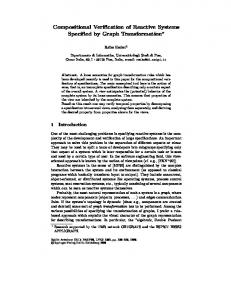


![Comparison of Identity Verification Systems - IDValidation.net [PDF]](https://m.moam.info/img/260x300/comparison-of-identity-verification-systems-idvali_649a7137098a9ef5168b47a4.jpg)