VERIFICATION OF CONTACT MODELING WITH COMSOL MULTIPHYSICS SOFTWARE Fabienne Pennec1, Hikmat Achkar1, David Peyrou1, Robert Plana1, Patrick Pons1, Fréderic Courtade2 1
LAAS-CNRS, Toulouse University 7, av. Du Colonel Roche, 31077 Toulouse cedex 4, France 2 CNES, Centre National d’Etudes Spatiales Service Laboratoires & Expertises 18 av E. Belin, 31401 Toulouse cedex 9, France
[email protected] (Fabienne Pennec) Abstract Contact analysis is a major concern in many applications such as metal forming, projectile impact, electrical relay, and addresses often multi-field effects (thermal, electromagnetic…). Due to the nonlinearity and difficulty in predicting the behaviour of the bodies coming into and go out of contact, we need software able to simulate a structural contact problem and couple it with other physics. The last version 3.3 of COMSOL Multiphysics allows the analysis of multiphysics contact problem and appears to be interesting. Being new and under development, COMSOL 3.3 needs therefore to be validated in terms of contact modeling. Only the cases of frictionless problem are considered. A static contact Hertz model and a model containing a rigid-flexible contact and a flexible-flexible contact are studied and describe the capabilities, advantages, originalities and drawbacks of COMSOL. A good user interface and the capabilities to couple all physics with facilities make attractive the software. However, contact algorithm implemented in COMSOL doesn’t allow the resolution of all contact problems. The more evident, like a Hertz contact can be solved efficiently with a reduced computational time. A problem containing an initial gap between two deformable surfaces requires more computational costs and solver fails to find a solution easily. The user has to spend enough time to set up the contact parameters. But it isn’t always evident to check these parameters to optimise the solution accuracy and the time of resolution. More investments have to be provided to improve the contact algorithms and to facilitate the user to choose the contact parameters. Keywords: Mechanical Contact, Augmented Lagrangian method, penalty factor, Hertz contact, convergence Fabienne Pennec received the mechanical degree engineering from ENSMM, Besançon, France in 2005 and is currently pursuing the PhD degree in LAAS-CNRS and in collaboration with the CNES, in reliability of low actuation voltage RF MEMS switches.
1
Introduction
As part of our study on the electrical contacts of RF MEMS micro switches, the need of multiphysics software offering a well developed solver to simulate mechanical contact problems coupled with other physics, with a reduced time of calculation and good accuracy on the results is a major concern. Contact problems are highly nonlinear and require significant computer resources to solve. One major problem is that the contact regions are generally not known. Depending on the loads, material, boundary conditions, and other factors, surfaces can come into contact and then be separated in a largely unpredictable and abrupt manner. In addition to this difficulty, many contact problems must also address many physics domains effects, such as the conductance of heat, electrical currents, and magnetic flux in the areas of contact. This need to combine mechanical simulation with other physical behaviours implies the need to use multiphysics software. COMSOL 3.3, new multiphysics software having a good interactive interface appears attractive. New features in structural mechanics module of the last version 3.3 were developed: surface-to-surface contact with and without friction 2D and 3D, augmented Lagrangian solver method, thermal contact and multiphysics contact. Being new and under development, COMSOL 3.3 needs therefore to be validated in terms of contact modeling. In this paper, only the normal contact forces are considered, as in the case of frictionless contact problem. First, contact solver is explained in order to run a contact problem as efficiently as possible and to avoid making solution convergence difficult. Next, a static Hertz contact problem is simulated with Comsol Multiphysics in the goal to validate the contact results by analytical values determined from Hertz theory. A second model consists of one rigid body in contact with a flexible structure. Another flexible body is added under the first. This model allows the validation of contact between rigid and flexible bodies on the one hand, and to validate the contact between both flexible bodies on the other hand. Lastly, an example of contact problem with multi-field effects is studied.
2 Contact modeling theory background in COMSOL 3.3 A brief description of contact algorithm is given to help the user to set up the contact parameters as efficiently as possible. Only the case of normal contact forces is approached, as in the case of frictionless contact. When modeling contact, structural parts that come into contact have to be defined and consisted of two sets of boundaries, a slave and a master domain [1]. The slave boundaries can’t penetrate the master boundaries. To solve the finite element analysis an optimal convergence for NewtonRaphson iteration is required and so augmented
Lagrangian method is implemented in COMSOL 3.3. This method is a combination of penalty and Lagrange multiplier methods [2]. It means a penalty method with penetration control. The advantages and disadvantages of both techniques are well known and discussed by Kikuchi and Oden [3], and Simo and Laursen [4]. Also, the system is solved by iteration from the determined displacement. These displacements caused by incremental loading, are stored and used to deform the structure to its current geometry. If the gap distance between the slave and master boundaries at a given equilibrium iteration is becoming negative, (the master boundary is penetrating the slave boundary), the user defined normal penalty factor pn is augmented with Lagrange multipliers for contact pressure Tn [2].
(1)
g is the gap (penetration), that is the distance between two existing nodes on master and slave boundaries, and pn is defined as a contact stiffness.
Fig.1 Evaluation of the gap distance between slave point and master point [5]
Normal penalty factor and initial value for the contact pressure have to be checked by the user [6]. We guess that if the penalty factor is set up too high, the iteration process is likely to fail in the first augmented iterations and if it is too low, the contact model is likely to converge but very too slowly. As for the initial contact pressure, if it is too low the parts might pass through each other in the first iterations, if it is too high they never come into contact. Therefore, the set up of both contact parameters are crucial for convergence of the model.
3
Static Hertz contact model
3.1
Contact modeling
A simple contact problem occurs when, for example, one elastic curved body with smooth surface comes in contact with no friction with an elastic plane smooth surface under static conditions [2]. The area of contact is a function of the applied load. With the change in
contact area with load, the extent of contact is a priori unknown, rendering the problem nonlinear. However, it is of a reversible nature due to the absence of nonconservative forces. Analytical solutions to frictionless elastic contact problem with simple geometries can be found in the literature. Heinrich Hertz was the first to treat successfully the problem of the contact of smooth elastic bodies under normal loading. He computed and checked by experiment the load distributions over the contact area.
Tab. 1 Material properties for the contact model Gold
Steel
E (MPa)
Young modulus
70000
210000
ν
Poisson ratio
0.44
0.3
P (MPa)
Applied pressure
500
The equations of Hertz theory are detailed below for small deformations.
Pmax Pressure P
2F = = Πa
FE * = ΠR
2 PE * Π
(2)
Where the combined elastic modulus E* is defined by
1 1 −ν 12 1 −ν 22 = + E* E1 E2
(3)
The contact length is given by
a=
4 FR 8 PR 2 = ΠE * ΠE *
(4)
Fig. 2 Static Hertz contact model
An elastic contact problem satisfying the Hertzian conditions is then simulated with Comsol Multiphysics [7, 8]. The objective is to validate the contact results by analytical values determined from the formulation of Hertz [9, 10]. The numerical model consists in a gold half-cylinder compressed on a rigid steel block as illustrated in figure 2. Both materials are assumed to be elastic, homogeneous and isotropic. Moreover, there is no friction and the problem consists of small deformations. Plane strain conditions are considered. Comsol has a good user software interface which facilitates contact modeling. 2D structure is drawn by the drawing interface and then a contact pair is chosen by the user by selecting a master boundary and a slave boundary (fig.3) in the model considering that the master (steel block material) has to be stiffer than the slave (gold half-cylinder material), the slave is meshed finer than the master and the master has to be concave and the slave convex rather than the opposite [1]. Then, both contact parameters, initial contact pressure and penalty factor, have to be defined in order to help the solver to solve the problem. The output parameters, maximum contact pressure at the interface and contact length, are simulated with COMSOL Multiphysics and then compared with the analytical maximum contact pressure and contact length calculated with Hertz theory.
a is contact length in the x-axis direction F is the applied load (load/length) P is the pressure applied on the top of half-cylinder Pmax is the maximum pressure (at x=0) R is the radius of the cylinder (50 mm)
Steel block
0
x axis
Fig. 3 Symmetric plane strain contact model as built in COMSOL 3.3
3.2
Results
Maximum contact pressure simulated with Comsol Multiphysics is evaluated to 4474 MPa and is in good agreement with the analytical maximum pressure of 4447 MPa within a difference of 0.6%. As for the contact length, Comsol evaluated it as 7.22mm while the analytical solution gave 7.16mm, that is a difference of 0.8% which is very satisfactory. Now the contact pressure as a function of x can be expressed as:
P ( x) = Pmax
⎛ ⎛ x ⎞2 ⎞ ⎜1 − ⎜ ⎟ ⎟ ⎜ ⎝a⎠ ⎟ ⎝ ⎠
(5)
The following graph (fig. 4) shows the distribution of contact pressure along the surface of contact, for both Comsol and analytical solutions. Both graphs are superposing and validating the contact simulation for a static Hertz contact problem for a reduced satisfying time of calculation.
4 Contact validation for rigiddeformable and deformable-deformable bodies 4.1
Model description
In practice, The Hertz theory is inadequate for treating the wide variety of technologically important problems. Without considering the case where components are required to transmit tangential force, the contact model can present, for example, large deformations, some minimal plastic deformation. It is obvious that the calculation becomes even more complicated. The studied model in this part consists in one rigid gold cylinder in contact with a flexible gold bridge. A second bridge is added under the first to create a contact between two flexible bodies. The plane strain problem is frictionless, gold material is homogeneous, elastic and isotropic. This model allows the validation of contact between rigid and flexible bodies on the one hand, and to validate the contact between both flexible bodies on the other hand. The 2D-contact model drawn in COMSOL 3.3 is illustrated on figure 5. A load force is applied on the rigid cylinder and causes the bridge deformation that comes into contact with the second flexible bridge. Two contact pairs are defined, one between the rigid cylinder and the deformable bridge and one between the two deformable bodies. Nevertheless, if the mesh type and size of both bridges are identical, a double contact pair can be defined. The symmetric master-slave method involves additional computational expense but increases accuracy.
Arc length (mm)
Fig. 4 Contact pressure (MPa) along the contact area for both the analytical (dotted line) and the COMSOL Multiphysics solution (continuous line) 3.3
Drawbacks
Another static contact problem of Hertz consists in a sphere in contact on a rigid flat plane. Solving this problem type with a 3D-model is limited due to limitation of memory. Memory is a major issue in 3D and it is also interessant to use an axisymmetric model. However, COMSOL software offers only plane strain, plane stress and solid stress-strain application mode for a contact model. The COMSOL contact modeling doesn’t yet support the axial symmetry study and this point has to be implemented in the next versions.
Fig.5 2D Numerical Contact Model as built in COMSOL 3.3 4.2
Convergence problem of the contact model
To solve the problem without friction but with an initial gap between both deformable gold bridges, a parametric analysis is performed on the applied force F to help the solver to converge and find a solution. The finer the mesh will be, the smaller the parametric step will be chosen. The drawbacks of this method are the additional computational time consumption. In addition, the finer the mesh is, more the solver has difficulties to find solution, whereas a sufficiently fine mesh size is needed in order to obtain accurate results. When the parts are not in contact initially, the solver
has difficulties to converge. It is important to take the time to set up the model, optimise the contact parameters to run as efficiently as possible. Both contact pair parameters have to be checked by the user. The penalty factor can help the solver to get started or to speed up the convergence. As for the initial contact pressure, it is important to have a good estimation of this as it is of major concern for the problem convergence. Nevertheless for complicated design, this estimation can be difficult to know. Once the solver fails to find a solution, no information in the error file is noted to mention the source of error and so it becomes difficult to regulate the parameters. If the compression is imposed by a prescribing displacement on the rigid cylinder, the solver succeeds in finding a solution for small displacements. For larger displacements, a solution is found (fig.6) without reaching the tolerance criterion, so it puts a question mark on the accuracy of the results and it won’t be possible to run a parametric analysis on the displacement.
surface of the block. Once the structural plane strain analysis is run, a contact area is defined as function of applied force or pressure, which allows the current to flow through. In figure 7 are illustrated the current lines of the contact model. Then it is possible to obtain an approximation of the contact resistance by extracting the electrical powers on the two subdomains between the two green sections. z x
Fig. 7 Illustration of the current lines obtained with a simulation in DC media conduction application mode It consists in performing in COMSOL Multiphysics a double integral of term A (eq. 7) on both subdomains, related to the gold cylinder on the one hand, and to the titanium block on the other hand. The current intensity being a known data in Comsol or easily extractable, the resistance is deduced on the two subdomains. The approximative contact resistance is the sum of both calculated resistances.
Fig.6 Numerical contact model deformation with a prescribed displacement of 0.5m. The color map corresponds to the Von Mises stresses from 0 (blue) to 4300 MPa (red). Therefore, it seems that contact solver implemented in COMSOL 3.3 contains faults and improvement in the contact algorithm is necessary to solve a large range of contact problem and avoid the user to spend such a time to set up the parameters up to obtain a convergence of the solver with a satisfying time of resolution.
5 Example of a multiphysics contact model The metal contacts are a crucial part of the RF MEMS switches since they introduce a contact resistance. To improve the reliability of electric contact microswitches, it can be interesting to evaluate the contact resistance with simulation tools. In this context, we need to test the capabilities of COMSOL 3.3 to couple electromagnetic mode with contact mechanical analysis. We consider again the classical Hertz contact model with a gold half-cylinder (5µm radius) in contact with a titanium block. A current density or a potential voltage is applied on the top surface of the half-cylinder, the ground being set to the bottom
Pn élec = ∫∫
A=
j ( x, z ) 2
j ( x, z ) 2
γn
γn
LdS = Rn i 2
L
(6)
(7)
i is the current intensity S is the section γn is the resistivity of subdomain n L is the thickness of the model (20 µm) j(x, z) is the current density and depends on the model coordinates Rn the resistance of subdomain n The graph 8 illustrates the extracted contact resistance as a function of the applied load (load/length). Tab. 2 material properties Gold
Titanium
E (MPa)
70000
40000
ν
0.44
0.36
ρ (kg/m3)
19300
4506
σ (S/m)
45.6e6
2.6e6
International Conference on Thermal, Mechanical and Multi-physics Simulation and Experiments in Micro-Electronics and Micro-Systems EuroSimE, pp. 520-524, 2007. [8] COMSOL33\doc, Contact and Friction Models : 2D Cylinder Roller Contact [9] H. Hertz, Über die Berührung fester elastischer Körper, Journal für die reine und angewandte. Mathematik 92, 156-171 (1881) Fig. 8 Extracted contact resistance (mΩ) as a function of the applied force (µN)
6
Conclusions
Finally, COMSOL Multiphysics 3.3 offers interesting capabilities, like the possibility to couple all physics with contact mechanical analysis or a good user interface which facilitates contact modeling. However, even if simple contact model can be solved efficiently with the software with a reduced time of computation, for more elaborate models with variable initial gap distance, the solver is limited in mechanical contact simulation and can become highly time consuming. Moreover, some drawbacks are added, as the fact that contact modeling in COMSOL 3.3 doesn't support axial symmetry stress-strain application mode, and doesn't support elasto-plastic materials like contact materials, although it is rare that contact material is sufficiently hard to avoid some minimal plastic deformation.
7
References
[1] COMSOL33\doc, Creating and Analyzing Models : Contact Pairs [2] A. Faraji, Elastic and Elastoplastic Contact Analysis using Boundary Elements and Mathematical Programming, Topics in Engineering, vol. 45, WIT Press UK 2005 [3] N. Kikuchi and J.T. Oden, Contact problems in elasticity: a study of variational inequalities and finite elements method, SIAM, Philadelphia, 1988 [4] J.C. Simo and T.A. Laursen, Augmented Lagrangian treatment of contact problems involving friction. Computers and Structures, 42, 1, 97-116, 1992. [5] COMSOL33\doc, Continuum Application Modes: Theory Background - Contact modeling [6] COMSOL33\doc, Continuum Application Modes : Application Mode Description – The contact page [7] H. Hachkar, F. Pennec, D. Peyrou, M. Al Ahmad, M. Sartor, R. Plana and P. Pons. Validation of simulation platform by comparing results and calculation time of different softwares. IEEE
[10] http://agregb1.dgm.enscachan.fr/Documents/TheorieTP/files/Contact.pdf [11] A. Curnier, Unilateral Contact: mechanical modeling. New developments in contact problems, Springer-Verlag:Berlin, pp. 1-54, 1999