in the real world, or that some information present in the real world is stored into the information system. We do not e
Verification of Query Completeness over Processes Simon Razniewski, Marco Montali, and Werner Nutt Free University of Bozen-Bolzano Dominikanerplatz 3 39100 Bozen-Bolzano {razniewski,montali,nutt}@inf.unibz.it
Abstract. Data completeness is an essential aspect of data quality, and has in turn a huge impact on the effective management of companies. For example, statistics are computed and audits are conducted in companies by implicitly placing the strong assumption that the analysed data are complete. In this work, we are interested in studying the problem of completeness of data produced by business processes, to the aim of automatically assessing whether a given database query can be answered with complete information in a certain state of the process. We formalize so-called quality-aware processes that create data in the real world and store it in the company’s information system possibly at a later point. We then show how one can check the completeness of database queries in a certain state of the process or after the execution of a sequence of actions, by leveraging on query containment, a well-studied problem in database theory.
1 Introduction Data completeness is an important aspect of data quality. When data is used in decisionmaking, it is important that the data is of good quality, and in particular that it is complete. This is particularly true in an enterprise setting. On the one hand, strategic decisions are taken inside a company by relying on statistics and business indicators such as KPIs. Obviously, this information is useful only if it is reliable, and reliability, in turn, is strictly related to quality and, more specifically, to completeness. Consider for example the school information system of the autonomous province of Bolzano in Italy, which triggered the research included in this paper. Such an information system stores data about schools, enrolments, students and teachers. When statistics are computed for the enrolments in a given school, e.g., to decide the amount of teachers needed for the following academic year, it is of utmost importance that the involved data are complete, i.e., that the required information stored in the information system is aligned with reality. Completeness of data is a key issue also in the context of auditing. When a company is evaluated to check whether its way of conducting business is in accordance to the law and to audit assurance standards, part of the external audit is dedicated to the analysis of the actual data. If such data are incomplete w.r.t. the queries issued during the audit, then the obtained answers do not properly reflect the company’s behaviour. There has been plenty of work on fixing data quality issues, especially for fixing incorrect data and for detecting duplicates [10,6]. However, some data quality issues cannot be automatically fixed. This holds in particular for incomplete data, as missing F. Daniel, J. Wang, and B. Weber (Eds.): BPM 2013, LNCS 8094, pp. 155–170, 2013. c Springer-Verlag Berlin Heidelberg 2013 �
156
S. Razniewski, M. Montali, and W. Nutt
data cannot be corrected inside a system, unless additional activities are introduced to acquire them. In all these situations, it is then a mandatory requirement to (at least) detect data quality issues, enabling informed decisions drawn with knowledge about which data are complete and which not. The key question therefore is how it is possible to obtain this completeness information. There has been previous work on the assessment of data completeness [12], however this approach left the question where completeness information come from largely open. In this work, we argue that, in the common situation where the manipulation of data inside the information system is driven by business processes, we can leverage on such processes to infer information about data completeness, provided that we suitably annotate the involved activities with explicit information about the way they manipulate data. A common source of data incompleteness in business processes is constituted by delays between real-world events and their recording in an information system. This holds in particular for scenarios where processes are carried out partially without support of the information system. E.g., many legal events are considered valid as soon as they are signed on a sheet of paper, but their recording in the information system could happen much later in time. Consider again the example of the school information system, in particular the enrolment of pupils in schools. Parents enroll their children at the individual schools, and the enrolment is valid as soon as both the parents and the school director sign the enrolment form. However, the school secretary may record the information from the sheets only later in the local database of the school, and even later submit all the enrolment information to the central school administration, which needs it to plan the assignment of teachers to schools, and other management tasks. In the BPM context, there have been attempts to model data quality issues, like in [7,14,2]. However, these approaches mainly discussed general methodologies for modelling data quality requirements in BPMN, but did not provide methods to asses their fulfilment. In this paper, we claim that process formalizations are an essential source for learning about data completeness and show how data completeness can be verified. In particular, our contributions are (1) to introduce the idea of extracting information about data completeness from processes manipulating the data, (2) to formalize processes that can both interact with the real-world and record information about the real-world in an information system, and (3) to show how completeness can be verified over such processes, both at design and at execution time. Our approach leverages on two assumptions related to how the data manipulation and the process control-flow are captured. From the data point of view, we leverage on annotations that suitably mediate between expressiveness and tractability. More specifically, we rely on annotations modeling that new information of a given type is acquired in the real world, or that some information present in the real world is stored into the information system. We do not explicitly consider the evolution of specific values for the data, as incorporating full-fledged data without any restriction would immediately make our problem undecidable, being simple reachability queries undecidable in such a rich setting [9,3,4]. From the control-flow point of view, we are completely orthogonal to process specification languages. In particular, we design our data completeness algorithms over (labeled) transition systems, a well-established mathematical structure to
Verification of Query Completeness over Processes
157
represent the execution traces that can by produced according to the control-flow dependencies of the (business) process model of interest. Consequently, our approach can in principle be applied to any process modeling language, with the proviso of annotating the involved activities. We are in particular interested in providing automated reasoning facilities to answer whether a given query can be answered with complete information given a target state or a sequence of activities. The rest of this paper is divided as follows. In Section 2, we discuss the scenario of the school enrolment data in the province of Bozen/Bolzano in detail. In Section 3, we discuss our formal approach, introducing quality-aware transition systems, process activity annotations used to capture the semantics of activities that interact with the real world and with an information system, and properties of query completeness over such systems. In Section 4, we discuss how query completeness can be verified over such systems at design time and at runtime, how query completeness can be refined and what the complexity of deciding query completeness is. The proofs of Proposition 1 and 2 and of Lemma 1 and 2 are available in the extended version available at Arxiv.org [13].
2 Example Scenario Consider the example of the enrollment to schools in the province of Bolzano. Parents can submit enrollment requests for their child to any school they want until the 1st of March. Schools then decide which pupils to accept, and parents have to choose one of the schools in which their child is accepted. Since in May the school administration wants to start planning the allocation of teachers to schools and take further decisions (such as the opening and closing of school branches and schools) they require the schools to process the enrollments and to enter them in the central school information system before the 15th of April. A particular feature of this process is that it is partly carried out with pen and paper, and partly in front of a computer, interacting with an underlying school information system. Consequently, the information system does not often contain all the information that hold in the real world, and is therefore incomplete. E.g., while an enrollment is legally already valid when the enrollment sheet is signed, this information is visible in the information system only when the secretary enters it into a computerised form. A BPMN diagram sketching the main phases of this process is shown in Fig. 1, while a simple UML diagram of (a fragment of) the school domain is reported in Fig. 2. These diagrams abstractly summarise the school domain from the point of view of the central administration. Concretely, each school implements a specific, local version of the enrolment process, relying on its own domain conceptual model. The data collected on a per-school basis are then transferred into a central information system managed by the central administration, which refines the conceptual model of Fig. 2. In the following, we will assume that such an information system represents information about children and the class they belong to by means of a pupil(pname, class, sname) relation, where pname is the name of an enrolled child, class is the class to which the pupil belongs, and sname is the name of the corresponding school.
158
S. Razniewski, M. Montali, and W. Nutt Parents
Schools
Submit enrolment applications
School Administration
Enrolment applications
Decide about enrolment requests
Record accepted enrolments
Generate statistics and assign resources
Enrolment deadline School information system
Fig. 1. BPMN diagram of the main phases of the school enrollment process
Parent
Child 0..2 1..* - name: String hasChild 0..* livesIn 1..1 Place - name: String
Class School Admin 0..* 0..1 - no: int belongsTo 1..1 0..* isAt managedBy 1..1 1..* School Branch locatedIn offers - name: String - type: String 0..* 0..* 1..* 1..1
Fig. 2. UML diagram capturing a fragment of the school domain
When using the statistics about the enrollments as compiled in the beginning of May, the school administration is highly interested in having correct statistical information, which in turn requires that the underlying data about the enrollments must be complete. Since the data is generated during the enrollment process, this gives rise to several questions about such a process. The first question is whether the process is generally designed correctly, that is, whether the enrollments present in the information system are really complete at the time they publish their statistics, or whether it is still possible to submit valid enrollments by the time the statistics are published. We call this problem the design-time verification. A second question is to find whether the number of enrollments in a certain school branch is already complete before the 15th of April, that is, when the schools are still allowed to submit enrolments (i.e., when there are school that still have not completed the second activity in the school lane of Fig. 1), which could be the case when some schools submitted all their enrollments but others did not. In specific cases the number can be complete already, when the schools that submitted their data are all the schools that offer the branch. We call this problem the run-time verification. A third question is to learn on a finer-grained level about the completeness of statistics, when they are not generally complete. When a statistic consists not of a single number but of a set of values (e.g. enrollments per school), it is interesting to know for which schools the number is already complete. We call this the dimension analysis.
3 Formalization We want to formalize processes as in Fig. 1, which both operate over data in the realworld (pen and paper) and record information about the real world in an information system. We therefore first introduce real-world databases and information system
Verification of Query Completeness over Processes
159
databases, and then annotate transition systems, which represent possible process executions, with effects to interact with the real-world or the information system database. 3.1 Real-World Databases and Information System Databases As common in database theory, we assume a set of constants dom and a fixed set Σ of relations, comprising the built-in relations < and ≤ over the rational numbers. We assume that dom is partitioned into the types of strings and rational numbers and that the arguments of each relation are typed. A database instance is a finite set of facts in Σ over dom. As there exists both the real world and the information system, in the following we model this with two databases: Drw called the real-world database, which describes the information that holds in the real world, and Dis , called the information system database, which captures the information that is stored in the information system. We assume that the stored information is always a subset of the real-world information. Thus, processes actually operate over pairs (Drw , Dis ) of real-world database and information system database. In the following, we will focus on processes that create data in the real world and copy parts of the data into the information system, possibly delayed. Example 1. Consider that in the real world, there are the two pupils John and Mary enrolled in the classes 2 and 4 at the Hofer School, while the school has so far only processed the enrollment of John in their IT system. Additionally it holds in the real world that John and Alice live in Bolzano and Bob lives in the city of Merano. The real-world database Drw would then be {pupil(John, 2, HoferSchool), pupil(Mary, 4, HoferSchool), livesIn(John, Bolzano), livesIn(Bob, Merano), livesIn(Alice, Bolzano)} while the information system database would be {pupil(John, 2, HoferSchool)}. When necessary, we annotate atoms with the database they belong to. So, pupilis (John, 4, HoferSchool) indicates a fact stored in the information system database. 3.2 Query Completeness For planning purposes, the school administration is interested in figures such as the number of pupils per class, school, profile, etc. Such figures can be extracted from relational databases via SQL queries using the COUNT keyword. In an SQL database with a table pupil(name, class, school), a query asking for the number of students per school would be written as: SELECT school, COUNT(name) as pupils_nr FROM pupil GROUP BY school.
(1)
In database theory, conjunctive queries were introduced to formalize SQL queries. A conjunctive query Q is an expression of the form Q( x¯) :− A1 , . . . , An , M, where x¯ are called the distinguished variables in the head of the query, A1 to An the atoms in the body of the query, and M is a set of built-in comparisons [1]. We denote the set of all variables that appear in a query Q by Var(Q). Common subclasses of conjunctive queries are linear conjunctive queries, that is, they do not contain a relational symbol twice, and relational conjunctive queries, that is, queries that do not use comparison
160
S. Razniewski, M. Montali, and W. Nutt
predicates. Conjunctive queries allow to formalize all single-block SQL queries, i.e., queries of the form “SELECT . . . FROM . . . WHERE . . .”. As a conjunctive query, the SQL query (1) above would be written as: Q p/s (schoolname, count(name)) :− pupil(name, class, schoolname)
(2)
In the following, we assume that all queries are conjunctive queries. We now formalize query completeness over a pair of a real-world database and an information system database. Intuitively, if query completeness can be guaranteed, then this means that the query over the generally incomplete information system database gives the same answer as it would give w.r.t. the information that holds in the real world. Query completeness is the key property that we are interested in verifying. A pair of databases (Drw , Dis ) satisfies query completeness of a query Q, if Q(Drw ) = Q(Dis ) holds. We then write (Drw , Dis ) |= Compl(Q). Example 2. Consider the pair of databases (Drw , Dis ) from Example 1 and the query Q p/s from above (2). Then, Compl(Q p/s ) does not hold over (Drw , Dis ) because Q(Drw ) = {(HoferSchool, 2)} but Q(Dis ) = {(HoferSchool, 1)}. A query for pupils in class 2 only, Qclass2 (n) :− pupil(n, 2, s), would be complete, because Q(Drw ) = Q(Dis ) = {John}. 3.3 Real-World Effects and Copy Effects We want to formalize the real-world effect of an enrollment action at the Hofer School, where in principle, every pupil that has submitted an enrolment request before, is allowed to enroll in the real world. We can formalize this using the following expression: pupilrw (n, c, HoferSchool) � requestrw (n, HoferSchool), which should mean that whenever someone is a pupil at the Hofer school now, he has submitted an enrolment request before. Also, we want to formalize copy effects, for example where all pupils in classes greater than 3 are stored in the database. This can be written with the following implication: pupilrw (n, c, s), c > 3 → pupilis (n, c, s), which means that whenever someone is a pupil in a class with level greater than three in the real world, then this fact is also stored in the information system. For annotating processes with information about data creation and manipulation in the real world Drw and in the information system Dis , we use real-world effects and copy effects as annotations. While their syntax is the same, their semantics is different. Formally, a real-world effect r or a copy effect c is a tuple (R( x¯, y¯ ), G( x¯, z¯)), where R is an atom, G is a set of atoms and built-in comparisons and x¯, y¯ and z¯ are sets of distinct variables. We call G the guard of the effect. The effects r and c can be written as follows: r : Rrw ( x¯, y¯ ) � ∃¯z : Grw ( x¯, z¯) c : Rrw ( x¯, y¯), Grw ( x¯, z¯) → Ris ( x¯, y¯ ) Real-world effects can have variables y¯ on the left side that do not occur in the condition. These variables are not restricted and thus allow to introduce new values. rw rw ¯) � A pair of real-world databases (Drw 1 , D2 ) conforms to a real-world effect R ( x¯, y rw rw rw rw ∃¯z : G ( x¯, z¯), if for all facts R (¯c1 , c¯ 2 ) that are in D2 but not in D1 it holds that there
Verification of Query Completeness over Processes
161
exists a tuple of constants c¯ 3 such that the guard Grw (¯c1 , c¯ 3 ) is in Drw 1 . The pair of rw databases conforms to a set of real-world effects, if each fact in Drw \ D 2 1 conforms to at least one real-word effect. If for a real-world effect there does not exist any pair of databases (D1 , D2 ) with D2 \ D1 � ∅ that conforms to the effect, the effect is called useless. Useless effects can be detected by checking whether the effect does not have unbound variables (¯y is empty) and whether Q( x¯) :− G( x¯, z¯) is contained in Q( x¯) :− R( x¯). In the following we only consider real-world effects that are not useless. The function copyc for a copy effect c = Rrw ( x¯, y¯), Grw ( x¯, z¯) → Ris ( x¯, y¯) over a realworld database Drw returns the corresponding R-facts for all the tuples that are in the answer of the query Pc ( x¯, y¯ ) :− Rrw ( x¯, y¯ ), Grw ( x¯, z¯) over Drw . For a set of copy effects CE, the function copyCE is defined by taking the union of the results of the individual copy functions. Example 3. Consider a real-world effect r that allows to introduce persons living in Merano as pupils in classes higher than 3 in the real world, that is, r = pupilrw (n, c, s) � c > 3, livesIn(n, Merano) and a pair of real-world databases using the database Drw from Example 1 as (Drw , Drw ∪{pupilrw (Bob, 4, HoferSchool)}. Then this pair conforms to the real-world effect r, because the guard of the only new fact pupilrw (Bob, 4, HoferSchool) evaluates to true: Bob lives in Merano and his class level is greater than 3. The pair (Drw , Drw ∪ {pupilrw (Alice, 1, HoferSchool)} does not conform to r, because Alice does not live in Merano, and also because the class level is not greater than 3. For the copy effect c = pupilrw (n, c, s), c > 3 → pupilis (n, c, s), which copies all pupils in classes greater equal 3, its output over the real-world database in Example 1 would be {pupilis (Mary, 4, HoferSchool)}. 3.4 Quality-Aware Transition Systems To capture the execution semantics of quality-aware processes, we resort to (suitably annotated) labelled transition systems, a common way to describe the semantics of concurrent processes by interleaving [5]. This makes our approach applicable for virtually every business process modelling language equipped with a formal underlying transition semantics (such as Petri nets or, directly, transition systems). Formally, a (labelled) transition system T is a tuple T = (S , s0 , A, E), where S is a set of states, s0 ∈ S is the initial state, A is a set of names of actions and E ⊆ S × A×S is a set of edges labelled by actions from A. In the following, we will annotate the actions of the transition systems with effects that describe interaction with the real-world and the information system. In particular, we introduce quality-aware transition systems (QATS) to capture the execution semantics of processes that change data both in the real world and in the information system database. Formally, a quality-aware transition system T¯ is a tuple T¯ = (T, re, ce), where T is a transition system and re and ce are functions from A into the sets of all real-world effects and copy effects, which in turn obey to the syntax and semantics defined in Sec. 3.3. Note that transition systems and hence also QATS may contain cycles.
162
S. Razniewski, M. Montali, and W. Nutt
Example 4. Let us consider two specific schools, the Hofer School and the Da Vinci School, and a (simplified version) of their enrolment process, depicted in BPMN in Fig. 3(a) (in parenthesis, we introduce compact names for the activities, which will be used throughout the example). As we will see, while the two processes are independent from each other from the control-flow point of view (i.e., they run in parallel), they eventually write information into the same table of the central information system. Let us first consider the Hofer School. In the first step, the requests are processed with pen and paper, deciding which requests are accepted and, for those, adding the signature of the school director and finalising other bureaucratic issues. By using relation requestrw (n, HoferSchool) to model the fact that a child named n requests to be enrolled at Hofer, and pupilrw (n, 1, HoferSchool) to model that she is actually enrolled, the activity pH is a real-world activity that can be annotated with the real-world effect pupilrw (n, 1, HoferSchool) � requestrw (n, HoferSchool). In the second step, the information about enrolled pupils is transferred to the central information system by copying all real-world enrolments of the Hofer school. More specifically, the activity rH can be annotated with the copy effect pupilrw (n, 1, HoferSchool) → pupilis (n, 1, HoferSchool). Let us now focus on the Da Vinci School. Depending on the amount of incoming requests, the school decides whether to directly process the enrolments, or to do an entrance test for obtaining a ranking. In the first case (activity pD), the activity mirrors that of the Hofer school, and is annotated with the real-world effect pupilrw (n, 1, DaVinci) � requestrw (n, DaVinci). As for the test, the activity tD can be annotated with a realworld effect that makes it possible to enrol only those children who passed the test: pupilrw (n, 1, DaVinci) � requestrw (n, DaVinci), testrw (n, mark), mark ≥ 6. Finally, the process terminates by properly transferring the information about enrolments to the central administration, exactly as done for the Hofer school. In particular, the activity rD is annotated with the copy effect pupilrw (n, 1, DaVinci) → pupilis (n, 1, DaVinci). Notice that this effect feeds the same pupil relation of the central information systems that is used by rH, but with a different value for the third column (i.e., the school name). Fig. 3(b) shows the QATS formalizing the execution semantics of the parallel composition of the two processes (where activities are properly annotated with the previously discussed effects). Circles drawn in orange with solid line represent execution states where the information about pupils enrolled at the Hofer school is complete. Circles in blue with double stroke represent execution states where completeness holds for pupils enrolled at the Da Vinci school. At the final, sink state information about the enrolled pupils is complete for both schools. 3.5 Paths and Action Sequences in QATSs Let T¯ = (T, re, ce) be a QATS. A path π in T¯ is a sequence t1 , . . . , tn of transitions such that ti = (si−1 , ai , si ) for all i = 1 . . . n. An action sequence α is a sequence a1 , . . . , am of action names. Each path π = t1 , . . . , tn has also a corresponding action sequence απ defined as a1 , . . . , an . For a state s, the set Aseq(s) is the set of the action sequences of all paths that end in s. Next we consider the semantics of action sequences. A development of an action rw sequence α = a1 , . . . , an is a sequence Drw 0 , . . . , Dn of real-world databases such that rw rw each pair (D j , D j+1 ) conforms to the effects re(α j+1 ). Note that Drw 0 can be arbitrary.
"Hofer" school
"Da Vinci" school
Verification of Query Completeness over Processes
do test
X
process enrolment requests
163
(tD)
X (pD)
register enrolment forms (rD)
process enrolment requests (pH)
register enrolment forms (rH)
tD
rH
pD
tD
pH tD
pD
rH
pH
rD
rD
pH
pD
(a)
rD rH
(b)
Fig. 3. BPMN enrolment process of two schools, and the corresponding QATS
rw is is For each development Drw 0 , . . . , Dn , there exists a unique trace D0 , . . . , Dn , which is a is sequence of information system databases D j defined as follows:
Disj
⎧ rw ⎪ ⎪ ⎨D j =⎪ ⎪ ⎩Dis ∪ copyCE(t ) (Drw ) j j−1 j
if j = 0 otherwise.
Note that Dis0 = Drw 0 does not introduce loss of generality and is just a convention. To start with initially different databases, one can just add an initial action that introduces data in all real-world relations. 3.6 Completeness over QATSs An action sequence α = a1 , . . . , an satisfies query completeness of a query Q, if for all is rw is developments of α it holds that Q is complete over (Drw n , Dn ), that is, if Q(Dn ) = Q(Dn ) holds. A path P in a QATS T¯ satisfies query completeness for Q, if its corresponding action sequence satisfies it. A state s in a QATS T¯ satisfies Compl(Q), if all action sequences in Aseq(s) (the set of the action sequences of all paths that end in s) satisfy Compl(Q). We then write s |= Compl(Q). Example 5. Consider the QATS in Figure 3(b) and recall that the action pH is annotated with the real-world effect pupilrw (n, 1, HoferSchool) � requestrw (n, HoferSchool), and action rH with the copy effect pupilrw(n, 1, HoferSchool) → pupilis(n, 1, HoferSchool). A path π = ((s0 , pH, s1 ), (s1 , rH, s2 )) has the corresponding action sequence (pH, rH). rw rw Its models are all sequences (Drw 0 , D1 , D2 ) of real-world databases (developments), rw where D1 may contain additional pupil facts at the Hofer school w.r.t. Drw 0 because rw of the real-world effect of action a1 , and Drw = D . Each such development has a 2 1 is is by definition, D = D because uniquely defined trace (Dis0 , Dis1 , Dis2 ) where Dis0 = Drw 0 1 0 no copy effect is happening in action a1 , and Dis2 = Dis1 ∪ copyce(a1 ) (Drw 1 ), which means that all pupil facts from Hofer school that hold in the real-world database are copied into the information system due to the effect of action a1 . Thus, the state s2 satisfies Compl(QHofer ) for a query QHofer(n) :− pupil(n, c, HoferSchool), because in all models of the action sequence the real-world pupils at the Hofer school are copied by the copy effect in action rH.
164
S. Razniewski, M. Montali, and W. Nutt
4 Verifying Completeness over Processes In the following, we analyze how to check completeness in a state of a QATS at design time, at runtime, and how to analyze the completeness of an incomplete query in detail. 4.1 Design-Time Verification When checking for query completeness at design time, we have to consider all possible paths that lead to the state in which we want to check completeness. We first analyze how to check completeness for a single path, and then extend our results to sets of paths. Given a query Q(¯z) :− R1 (t¯1 ), . . . , Rn (t¯n ), M, we say that a real-world effect r is risky rw w.r.t. Q, if there exists a pair of real-world databases (Drw 1 , D2 ) that conforms to r and rw rw where the query result changes, that is, Q(D1 ) � Q(D2 ). Intuitively, this means that real-world database changes caused by r can influence the query answer and lead to incompleteness, if the changes are not copied into the information system. Proposition 1 (Risky effects). Let r be the real-world effect R( x¯, y¯) � G1 ( x¯, z¯1 ), Q be the query Q :− R1 (t¯1 ), . . . , Rn (t¯n ), M and v¯ = Var(Q). Then r is risky wrt. Q if and only if the following formula is satisfiable: �� � � � G1 ( x¯, z¯1 ) ∧ Ri (t¯i ) ∧ M ∧ ( x¯, y¯ ) = t¯i Ri =R
i=1...n
Example 6. Consider the query Q(n) :− pupil(n, c, s), livesIn(n, Bolzano) and the realworld effect r1 = pupil(n, c, s) � c = 4, which allows to add new pupils in class 4 in the real world. Then r1 is risky w.r.t. Q, because pupils in class 4 can potentially also live in Bolzano. Note that without integrity constraints, actually most updates to the same relation will be risky: if we do not have keys in the database, a pupil could live both in Bolzano and Merano and hence an effect r2 = pupil(n, c, s) � livesIn(n, Merano) would be risky w.r.t. Q, too. If there is a key defined over the first attribute of livesIn, then r2 would not be risky, because adding pupils that live in Merano would not influence the completeness of pupils that only live in Bolzano. We say that a real-world effect r that is risky w.r.t. a query Q is repaired by a set of rw copy effects {c2 , . . . , cn }, if for any sequence of databases (Drw 1 , D2 ) that conforms to r rw rw rw it holds that Q(D2 ) = Q(D1 ∪ copyc1 ...cn (D2 )). Intuitively, this means that whenever we introduce new facts via r and apply the copy effects afterwards, all new facts that can change the query result are also copied into the information system. Proposition 2 (Repairing). Consider the query Q :− R1 (t¯1 ), . . . Rn (t¯n ), M, let v¯ = Var(Q), a real-world effect R( x¯, y¯) � G1 ( x¯, z¯1 ) and a set of copy effects {c2 , . . . , cm }. Then r is repaired by {c2 , . . . , cm } if and only if the following formula is valid:
�
� ∀ x¯, y¯ : ∃¯z1 , v¯ : G1 ( x¯, z¯1 ) ∧ Ri (t¯i ) ∧ M ∧ ( x¯, y¯ ) = t¯i =⇒ ∃¯z j : G j ( x¯, z¯ j ) i=1...n
Ri =R
j=2...m
This implication can be translated into a problem of query containment, a well-studied topic in database theory [11,8,15,12]. In particular, for a query
Verification of Query Completeness over Processes
165
Q(¯z) :− R1 (t¯1 ), . . . , Rn (t¯n ), we define the atom-projection of Q on the i-th atom as Qπi ( x¯) :− R1 (t¯1 ), . . . , Rn (t¯n ), x¯ = t¯i . Then, for a query Q and a relation R, we define the R-projection of Q, written QR , as the union of all the atom-projections of atoms that use � the relation symbol R, that is, Ri =R Qπi . For a real-world effect r = R( x¯, y¯) � G( x¯, z¯), we define its associated query Pr as Pr ( x¯, y¯ ) :− R( x¯, y¯), G( x¯, z¯). Corollary 1 (Repairing and query containment). Let Q be a query, α = a1 , . . . an be an action sequence, ai be an action with a risky real-world effect r, and {c1 , . . . , cm } be the set of all copy effects of the actions ai+1 . . . an . Then r is repaired, if and only if it holds that Pr ∩ QR ⊆ Pc1 ∪ . . . ∪ Pcm . Intuitively, the corollary says that a risky effect r is repaired, if all data that is introduced by r that can potentially change the result of the query Q are guaranteed to be copied into the information system database by the copy effects c1 to cn . The corollary holds because of the direct correspondence between conjunctive queries and relational calculus [1]. We arrive at a result for characterizing query completeness wrt. an action sequence: Lemma 1 (Action sequence completeness). Let α be an action sequence and Q be a query. Then α |= Compl(Q) if and only if all risky effects in α are repaired. Before discussing complexity results in Section 4.4, we show that completeness entailment over action sequences and containment of unions of queries have the same complexity. A query language is defined by the operations that it allows. Common sublanguages of conjunctive queries are, e.g., queries without arithmetic comparisons (socalled relational queries), or queries without repeated relation symbols (so-called linear queries). For a query language L, we call EntC(L) the problem of deciding whether an action sequence α entails completeness of a query Q, where Q and the real-world effects and the copy effects in α are formulated in language L. Also, we call ContU(L) the problem of deciding whether a query is contained in a union of queries, where all are formulated in the language L. Theorem 1. Let L be a query languages. Then EntC(L) and ContU(L) can be reduced to each other in linear time. Proof. “⇒”: Consider the characterization shown in Lemma 1. For a fixed action sequence, the number of containment checks is the same as the number of the real-world effects of the action sequence and thus linear. “⇐”: Consider a containment problem Q0 ⊆ Q1 ∪ . . . ∪ Qn , for queries in a language L. Then we can construct a QATS T¯ = (S , s0 , A, E, re, ce) over the schema of the queries together with a new relation R with the same arity as the queries where S = {s0 , s1 , s2 }, � A = {a1 , a2 }, re(a1 ) = {Rrw ( x¯) � Q0 ( x¯)} and ce(a2 ) = i=1...n {Qi ( x¯) → Ris ( x¯)}. Now, the action sequence a1 , a2 satisfies a query completeness for a query Q� ( x¯) :− R( x¯) exactly if Q0 is contained in the union of the queries Q1 to Qn , because only in this case the real-world effect at action a1 cannot introduce any facts into Drw 1 of a development of � � a1 , a2 , which are not copied into Dis2 by one of the effects of the action a2 . We discuss the complexity of query containment and hence of completeness entailment over action sequences more in detail in Section 4.4.
166
S. Razniewski, M. Montali, and W. Nutt
So far, we have shown how query completeness over a path can be checked. To verify completeness in a specific state, we have to consider all paths to that state, which makes the analysis more difficult. We first introduce a lemma that allows to remove repeated actions in an action sequence: Lemma 2 (Duplicate removal). Let α = α1 , a˜ , α2 , a˜ , α3 be an action sequence with a˜ as repeated action and let Q be a query. Then α satisfies Compl(Q) if and only if α� = α1 , α2 , a˜ , α3 satisfies Compl(Q). The lemma shows that our formalism can deal with cycles. While cycles imply the existence of sequences of arbitrary length, the lemma shows that we only need to consider sequences where each action occurs at most once. Intuitively, it is sufficient to check each cycle only once. Based on this lemma, we define the normal action sequence of a path π as the action sequence of π in which for all repeated actions all but the last occurrence are removed. Proposition 3 (Normal action sequences). Let T¯ = (T, re, ce) be a QATS, Π be the set of all paths of T¯ and Q be a query. Then 1. for each path π ∈ Π, its normal action sequence has at most the length | A |, |A| |A|! 2. there are at most Σk=1 (|A|−k)! < (| A | +1)! different normal forms of paths, 3. for each path π ∈ Π, it holds that π |= Compl(Q) if its normal action sequence α� satisfies Compl(Q). The first two items hold because normal action sequences do not contain actions twice. The third item holds because of Lemma 2, which allows to remove all but the last occurrence of an action in an action sequence without changing query completeness satisfaction. Before arriving at the main result, we need to show that deciding whether a given normal action sequence can actually be realized by a path is easy: Proposition 4. Given a QATS T¯ , a state s and a normal action sequence α. Then, deciding whether there exists a path π that has α as its normal action sequence and that ends in s can be done in polynomial time. The reason for this proposition is that given a normal action sequence α = a1 , . . . , an , one just needs to calculate the states reachable from s0 via the concatenated expression (a1 , . . . , an )+ , (a2 , . . . , an )+ , . . . , (an−1 , an )+ , (an )+ . This expression stands exactly for all action sequences with α as normal sequence, because it allows repeated actions before their last occurrence in α. Calculating the states that are reachable via this expression can be done in polynomial time, because the reachable states S nreach can be calculated reach iteratively for each component (ai , . . . , an )+ as S ireach from the reachable states S i−1 + until the previous component (ai−1 , . . . , an ) by taking all states that are reachable from reach via one or several actions in {ai , . . . , an }, which can be done with a a state in S i−1 linear-time graph traversal such as breadth-first or depth-first search. Since there are only n such components, the overall algorithm works in polynomial time. Theorem 2. Given a QATS T¯ and a query Q, both formulated in a query language L, checking “s �|= Compl(Q)?” can be done using a nondeterministic polynomial-time Turing machine with a ContU(L)-oracle.
Verification of Query Completeness over Processes
167
Sign enrolment forms
X
X Record signed enrolment forms
School information system
Fig. 4. Simplified BPMN process for the everyday activity of a secretary in a school
Proof. If s �|= Compl(Q), one can guess a normal action sequence α, check by Prop. 4 in polynomial time that there exists a path π from s0 to s with α as normal action sequence, and by Thm. 1 verify using the ContU(L)-oracle that α does not satisfy Compl(Q). � � We discuss the complexity of this problem in Section 4.4 4.2 Runtime Verification Taking into account the concrete activities that were carried out within a process can allow more conclusions about completeness. As an example, consider that the secretary in a large school can perform two activities regarding the enrollments, either he/she can sign enrollment applications (which means that the enrollments become legally valid), or he/she can record the signed enrollments that are not yet recorded in the database. For simplicity we assume that the secretary batches the tasks and performs only one of the activities per day. A visualization of this process is shown in Fig. 4. Considering only the process we cannot draw any conclusions about the completeness of the enrollment data, because if the secretary chose the first activity, then data will be missing, however if the secretary chose the second activity, then not. If however we have the information that the secretary performed the second activity, then we can conclude that the number of the currently valid enrollments is also complete in the information system. Formally, in runtime verification we are given a path π = t1 , . . . , tn that was executed so far and a query Q. Again the problem is to check whether completeness holds in the current state, that is, whether all developments of π satisfy Compl(Q). Corollary 2. Let π be a path in a QATS and Q be a query, such that both Q and the real-world effects and the copy effects in the actions of π are formulated in a query language L. Then “π |= Compl(Q)?” and ContU(L) can be reduced to each other in linear time. The corollary follows directly from Theorem 1 and the fact that a path satisfies completeness if and only if its action sequence satisfies completeness. Runtime verification becomes more complex when also the current, concrete state of the information system database is explicitly taken into account. Given the current state D of the database, the problem is then to check whether all the developments of π in which Disn = D holds satisfy Compl(Q). In this case repairing of all risky actions is a sufficient but not a necessary condition for completeness: Example 7. Consider a path (s0 , a1 , s1 ), (s1 , a2 , s2 ), where action a1 is annotated with the copy effect requestrw (n, s) → requestis (n, s), action a2 with the real-world effect
168
S. Razniewski, M. Montali, and W. Nutt
Fig. 5. Visualization of the dimension analysis of Example 8
pupilrw (n, c, s) � requestrw (n, s), a database Dis2 that is empty, and consider a query Q(n) :− pupil(n, c, s), request(n, s). Then, the query result over Dis2 is empty. Since the relation request was copied before, and is empty now, the query result over any realworld database must be empty too, and therefore Compl(Q) holds. Note that this cannot be concluded with the techniques introduced in this work, as the real-world effect of action a2 is risky and is not repaired. The complexity of runtime verification w.r.t. a concrete database instance is still open. 4.3 Dimension Analysis When at a certain timepoint a query is not found to be complete, for example because the deadline for the submissions of the enrollments from the schools to the central school administration is not yet over, it becomes interesting to know which parts of the answer are already complete. Example 8. Consider that on the 10th of April, the schools “Hofer” and “Da Vinci” have confirmed that they have already submitted all their enrollments, while “Max Valier” and “Gherdena” have entered some but not all enrollments, and other schools did not enter any enrollments so far. Then the result of a query asking for the number of pupils per school would look as in Fig. 5 (left table), which does not tell anything about the trustworthiness of the result. If one includes the information from the process, one could highlight that the data for the former two schools is already complete, and that there can also be additional schools in the query result which did not submit any data so far (see right table in Fig. 5). Formally, for a query Q a dimension is a set of distinguished variables of Q. Originally, dimension analysis was meant especially for the arguments of a GROUP BY expression in a query, however it can also be used with other distinguished variables of a query. Assume a query Q( x¯) :− B( x¯, y¯ ) cannot be guaranteed to be complete in a specific state of a process. For a dimension w¯ ⊆ x¯, the analysis can be done as follows: ¯ :− B( x¯, y¯) over Dis . 1. Calculate the result of Q� (w) � is 2. For each tuple c¯ in Q (D ), check whether s, Dis |= Compl(Q[w/¯ ¯ c]). This tells whether the query is complete for the values c¯ of the dimension. 3. To check whether further values are possible, one has to guess a new value c¯ new for the dimension and show that Q[w/¯ ¯ cnew ] is not complete in the current state. For the guess one has to consider only the constants in the database plus a fixed set of new constants, hence the number of possible guesses is polynomial for a fixed dimension v¯ .
Verification of Query Completeness over Processes Query/QATS language L
Complexity of ContU(L) and EntC(L) (“π |= Compl(Q)”?)
Complexity of “s |= Compl(Q)”?
Linear relational queries Linear conjunctive queries
PTIME coNP-complete
Relational conjunctive queries Relational conjunctive queries over databases with finite domains
NP-complete
in coNP coNP-complete in Π2P
Π2P -complete
Π2P -complete
Π2P -complete
Π2P -complete
in PSPACE
in PSPACE
Conjunctive queries with comparisons Relational conjunctive queries over databases with keys and foreign keys
169
Fig. 6. Complexity of design-time and runtime verification for different query languages
Step 2 corresponds to deciding for each tuple with a certain value in Q(Dis ), whether it is complete or not (color red or green in Fig. 5, right table), Step 3 to deciding whether there can be additional values (bottom row in Fig. 5, right table). 4.4 Complexity of Completeness Verification In the previous sections we have seen that completeness verification can be solved using query containment. Query containment is a problem that has been studied extensively in database research. Basically, it is the problem to decide, given two queries, whether the first is more specific than the second. The results follow from Theorem 1 and 2, and are summarized in Figure 6. We distinguish between the problem of runtime verification, which has the same complexity as query containment, and design-time verification, which, in principle requires to solve query containment exponentially often. Notable however is that in most cases the complexity of runtime verification is not higher than the one of design-time verification. The results on linear relational and linear conjunctive queries, i.e., conjunctive queries without selfjoins and without or with comparisons, are borrowed from [12]. The result on relational queries is reported in [15], and that on conjunctive queries from [11]. As for integrity constraints, the result for databases satisfying finite domain constraints is reported in [12] and for databases satisfying keys and foreign keys in [8].
5 Conclusion In this paper we have discussed that data completeness analysis should take into account the processes that manipulate the data. In particular, we have shown how process models can be annotated with effects that create data in the real world and effects that copy data from the real world into an information system. We have then shown how one can verify the completeness of queries over transition systems that represent the execution semantics of such processes. It was shown that the problem is closely related to the problem of query containment, and that more completeness can be derived if the run of the process is taken into account. In this work we focussed on the process execution semantics in terms of transition systems. The next step is to realize a demonstration system to annotate high-level business process specification languages (such as BPMN or YAWL), extract the underlying quality-aware transition systems, and apply the techniques here presented to check
170
S. Razniewski, M. Montali, and W. Nutt
completeness. Also, we intend to face the open question of completeness verification at runtime taking into account the actual database instance. Acknowledgements. This work was partially supported by the ESF Project 2-2992010 “SIS - Wir verbinden Menschen”, and by the EU Project FP7-257593 ACSI. We are thankful to Alin Deutsch for an invitation that helped initiate this research, and to the anonymous reviewers for helpful comments.
References 1. Abiteboul, S., Hull, R., Vianu, V.: Foundations of Databases. Addison-Wesley (1995) 2. Bagchi, S., Bai, X., Kalagnanam, J.: Data quality management using business process modeling. In: IEEE International Conference on Services Computing, SCC 2006 (2006) 3. Bagheri Hariri, B., Calvanese, D., De Giacomo, G., De Masellis, R., Felli, P.: Foundations of relational artifacts verification. In: Rinderle-Ma, S., Toumani, F., Wolf, K. (eds.) BPM 2011. LNCS, vol. 6896, pp. 379–395. Springer, Heidelberg (2011) 4. Bagheri Hariri, B., Calvanese, D., De Giacomo, G., Deutsch, A., Montali, M.: Verification of relational data-centric dynamic systems with external services. In: PODS (2013) 5. Baier, C., Katoen, J.P.: Principles of Model Checking. The MIT Press (2008) 6. Bilenko, M., Mooney, R.J.: Adaptive duplicate detection using learnable string similarity measures. In: ACM SIGKDD, pp. 39–48 (2003) 7. Bringel, H., Caetano, A., Tribolet, J.M.: Business process modeling towards data quality: A organizational engineering approach. In: ICEIS, vol. (3) (2004) 8. Calì, A., Lembo, D., Rosati, R.: Query rewriting and answering under constraints in data integration systems. In: IJCAI 2003, pp. 16–21 (2003) 9. Damaggio, E., Deutsch, A., Hull, R., Vianu, V.: Automatic verification of data-centric business processes. In: Rinderle-Ma, S., Toumani, F., Wolf, K. (eds.) BPM 2011. LNCS, vol. 6896, pp. 3–16. Springer, Heidelberg (2011) 10. Hernández, M.A., Stolfo, S.J.: Real-world data is dirty: Data cleansing and the merge/purge problem. Data Mining and Knowledge Discovery 2(1), 9–37 (1998) 11. van der Meyden, R.: The complexity of querying indefinite data about linearly ordered domains. In: PODS, pp. 331–345 (1992) 12. Razniewski, S., Nutt, W.: Completeness of queries over incomplete databases. In: VLDB (2011) 13. Razniewski, S., Montali, M., Nutt, W.: Verification of query completeness over processes [Extended version] (2013), http://arxiv.org/abs/1306.1689 14. Rodríguez, A., Caro, A., Cappiello, C., Caballero, I.: A BPMN extension for including data quality requirements in business process modeling. In: Mendling, J., Weidlich, M. (eds.) BPMN 2012. LNBIP, vol. 125, pp. 116–125. Springer, Heidelberg (2012) 15. Sagiv, Y., Yannakakis, M.: Equivalence among relational expressions with the union and difference operation. In: VLDB, pp. 535–548 (1978)