Christopher Davis, Barbara Brown, Randy Bullock, Michael Chapman, Kevin. Manning, Rebecca Morss, and Agnes Takacs. National Center for Atmospheric ...
17.4 Verification Techniques Appropriate for Cloud-resolving NWP Models
By
Christopher Davis, Barbara Brown, Randy Bullock, Michael Chapman, Kevin Manning, Rebecca Morss, and Agnes Takacs National Center for Atmospheric Research Boulder, Colorado
1. Verification of Discrete Phenomena Verification is a critical component of the development and use of forecasting systems. Ideally, verification should play a role in monitoring the quality of forecasts, provide feedback to developers and forecasters to help improve forecasts, and provide meaningful information to forecast users to apply in their decisionmaking processes. In addition, as noted by Mahoney et al. (2002) forecast verification can help to identify differences among forecasts. Finally, because forecast quality is intimately related to forecast value, albeit through relationships that are sometimes quite complex, verification has an important role to play in assessments of the value of particular types of forecasts (Murphy 1993). In recent years forecasting approaches have become more complex and have been applied on finer scales. Unfortunately, traditional approaches for the verification of spatial forecasts, including QPFs and convective forecasts, are inadequate to meet current needs. Typically, verification techniques 1
have been based on simple grid overlays in which the forecast grid is matched to an observation grid or set of observation points. From these overlays, counts of forecast/observation (Yes/No) pairs are computed, to complete the standard 2x2 contingency table. The counts in this table can be used to compute a variety of verification measures and skill scores, such as the Probability of Detection (POD), False Alarm Ratio (FAR), Critical Success Index (CSI), and Equitable Threat Score (ETS) (e.g., Doswell et al. 1990; Wilks 1995). An important concern associated with use of this approach is that it is difficult to diagnose particular errors in the forecasts to provide meaningful information that can be used to improve the forecasts or provide guidance to forecast users. Figure 1 illustrates some of the difficulties associated with diagnosing forecast errors using standard verification statistics. This figure shows five examples of forecast/observation pairs, with the forecasts and observations represented as areas. For a forecast user, cases a-d clearly demonstrate four different types or levels of “goodness”:
The National Center for Atmospheric Research is sponsored by the National Science Foundation.
(a) appears to be a fairly good forecast, just offset somewhat to the right; (b) is a poorer forecast since the location error is much larger than for (a); (c) is a case where the forecast area is much too large and is offset to the right; (d) shows a situation where the forecast is both offset and has the wrong shape. Of the four (a)
(b) O F
O
F
O
F
F
(d) O
(c) (e) O
F
Figure 1: Schematic example of various forecast and observation combinations.
examples, it appears that case (a) is the “best”. Given the perceived differences in performance, it is dismaying to note that all of the first four examples have identical basic verification statistics: POD=0, FAR=1, CSI=0. Thus, the verification technique is insensitive to differences in location and shape errors. Similar insensitivity could be shown to be associated with timing errors. Moreover, example (e) – which could be considered a very poor forecast from a variety of points of view – actually has some skill (POD, CSI >0), suggesting it is a better forecast than the one depicted in example (a). The present paper presents an object-oriented verification approach that more directly addresses the skill of fine scale forecasts than do traditional measures oriented approaches. With the
“object-oriented” approach, forecast and observed precipitation areas are reduced to regions of interest that can be compared to one another in a meaningful way. Ebert and McBride (2000, hereafter EM) were among the first to explore defining and verifying rainfall using objects labeled contiguous rainfall areas (CRAs). Their method identifies rainfall areas in both forecasts and observations, and it determines displacement errors and other parameters for matched regions. The accumulated statistics for errors in position can be constructed and biases, mean error, etc., computed. In broad terms the method we have developed is complementary to EM’s approach. Our means of identifying rain areas differs substantially from that presented in EM and we believe it is instructive to examine statistics of rainfall derived from different methods owing to the relative absence of object-based verification techniques found in the literature (and practiced in operational prediction centers). Our system is designed to be flexible enough to apply to any forecast system, in other words, it considers a range of scales for rain areas such that matching in the majority of instances is possible. In this paper, we will consider two sets of forecasts, produced by the Weather Research and Forecast model (WRF), one using a 22km grid covering the continental U.S. (CONUS), the other using a 4-km grid covering the central U.S. These two sets of forecasts illustrate the challenges of verification of rainfall forecasts on these different scales. In addition, we consider statistics of the rain areas themselves, without regard to matching, in accord with the well-documented limited predictability of rainfall, especially convective
precipitation. Thus, the applicability of our method is not restricted to quasipredictable situations. It should be kept in mind, however, that no single verification approach can yield complete information about the quality of forecasts due to the complexity of numerical models and incompleteness and errors inherent within observations. Thus, it is crucial that interpretations of model performance based on our method be viewed jointly with results from other methods. Examples of this important synergy will be discussed. Following a short summary of the verification problem, this article provides a detailed description of the verification methodology (Section 2). Several examples of applications of the approach are described in Section 3, and, along with a summary of results, the critical future directions are outlined in Section 4. 2. Methodology for Verification of Rain a. Concept As demonstrated in the previous section, one of the downfalls of standard verification approaches is that they often do not provide results that are consistent with subjective perceptions of the quality of a forecast (e.g., Fig. 1; Ebert 2003). While subjective verification in general cannot provide consistent and meaningful results for more than a handful of cases, it would be desirable to mimic some attributes of human capability in determining the “goodness” of the forecasts. Thus, our approach objectively identifies “objects” in the forecast and observed fields that are relevant to a human observer. These objects can then be described geometrically, and relevant attributes of
forecast and observed objects can be compared. These attributes include items such as location, shape, orientation, and size, depending on the user of the verification information. b. Data While our methodology is intended for a variety of forecast systems and observation sources, the present application considers precipitation forecasts from the Weather Research and Forecast (WRF) model (Michalakes et al. 2001). Forecasts from this model have been routinely produced at NCAR March 2001. The archive of real-time WRF precipitation forecasts includes 3hourly accumulations from a twicedaily, 48-h forecast on a 22-km mesh covering the continental United States (CONUS) and immediately adjacent waters of the Atlantic and Pacific Oceans (Fig. 2), and a daily 36 h forecast on a 4-km sub-CONUS grid. The time period covered by the coarser-resolution forecasts is July-August, 2001; the period covered by finer resolution is May13 – July 10, 2003, roughly coincident with the Bow Echo and MCV Experiment (BAMEX, see Weisman et al. 2003, elsewhere in this volume, and Done et al. 2003). We have chosen to use the NCEP Stage IV analysis as verification data. This analysis, which combines information from radar and gauge reports, is produced hourly in real-time on a 4-km CONUS grid. Some of the difficulties associated with using the Stage IV analysis include limited quality control and spotty coverage, especially over the mountainous western United States. To reduce observational uncertainty somewhat, we will mainly focus on precipitation systems to the east
of the Rocky Mountains. It will also turn out that biases in the predictions or observed estimates of rainfall do not greatly affect the determination of rainfall areas, but do affect the statistical distributions of rainfall inside the areas. Difficulties associated with precipitation estimation are partly the motivation for considering area and intensity separately in verification. For both the 22-km and 4-km WRF datasets, the Stage IV precipitation fields are interpolated to the model grid. The procedure averages all Stage IV grid boxes within each model grid box, accounting for instances when only a portion of an Stage IV grid box overlaps a model grid box. c. Identifying and Characterizing Rain Areas i. Overview Our verification approach involves several steps. First, the data field is convolved with an appropriate shape (cylinders are usually used unless some special feature in the data is being sought). Convolution is tantamount to spatial smoothing. It simply replaces the precipitation value at a point with its average over the area with a simple geometric shape (i.e. a disk) whose centroid is located at that point. Second, the convolved field is thresholded. This allows object boundaries to be detected. Thresholding without convolving does not result in object boundaries that are similar to those a human would draw – many objects would be filled with holes of various sizes, and the boundaries would be more jagged than human-rendered outlines. Convolution and thresholding also fills in most holes in the regions of interest and creates outside boundaries that enclose regions with a small amount
of room to spare – the same way a human would outline a region. Thresholds can be tuned to distinguish rain areas of greater size and intensity from those that are weaker and more isolated. The result of convolution and thresholding is a binary mask placed over the precipitation field with local, contiguous patches surrounded by regions of zero value. Note however, that the original precipitation values are retained and their statistics within each patch can be examined. Third, objects in the same field may be "associated" into simple geometric shapes. This is done both in the forecast and in the observed fields. The purpose is to create objects with relatively simple shapes such that aspect ratio, angle (orientation) and other properties have unambiguous interpretation. Geometric simplicity also allows numerical rotation of objects on a grid with no distortion of the shape due to finite grid size. Measures of the “goodness” of fit are calculated and can be examined to make sure that the simple shapes retain essential charactistics of the original objects. ii. Object properties Once objects have been “found” they can be assigned various properties for purposes of categorization and evaluation. Object properties currently in use include the following: • First and higher moments: These are used to calculate many of the other object characteristics listed below. In addition, they are of interest in their own right as an efficient summary of object size and internal intensity distribution. • Area: A simple measure of an object's size.
•
•
•
Centroid: One may imagine the centroid as a “center of mass” for the object. It is characterized by two scalar values – either lat/lon or grid x/y coordinates. Vector differences between the centroids of forecast and observed objects can reveal systematic location biases in the forecast. Axis angle: A line drawn through the centroid of an object to best characterize the overall direction or orientation of an object is another useful object descriptor. For example, storm systems off of a coastline often are approximately aligned with the coast, and differences in orientation between forecast and observed shapes can reveal another kind of bias. Note that the line drawn in this way is not the typical “least-squares” line fit. For simple shapes such as an ellipse, the axis angle is parallel to the major axis. For a rectangle, it is parallel to the longer sides. Curvature: Fitting a circular arc to an object instead of a line gives a measure of the object's overall deviation from straightness. The reciprocal of the radius of the fitted arc is taken as the measure of object curvature.
iii. Merging and Matching rules Current rules used to match observed and forecast objects use closest distance between centroids and difference in axis angle as indicators for object merging. If these two parameters are within a set range of values, objects are merged – otherwise they are not. Note that object matching consists of two parts. First, in a single field (either forecast or observation) objects may be
matched to form composite objects. Object properties are then recalculated for this composite object. Second, forecast objects and observed objects are matched according to a similar scheme (though perhaps with different thresholds) to determine forecast errors and biases. In addition, a third type of matching is possible: Objects in a single field at one time can be matched with objects in the same field at a different time. This analysis makes feasible the tracking of objects over time and evaluation of object lifetimes. Rules for matching adopted thus far are rather simple, but more complicated rules, accounting for more factors considered when humans subjectively match rain areas, will be considered in future work. For particular examples of the rain areas derived from our methodology, the reader is referred to Chapman et al. (2003), elsewhere in this volume. d. Outcomes The object-oriented approach to verification of QPFs and convective forecasts allows the diagnostic evaluation of many characteristics or attributes of the quality of these forecasts. In some cases different attributes of interest may be specified for different users of the verification information, depending on their interests. For example, forecast model developers may be interested in diagnosing characteristics that will help lead to improvements in the forecasts (e.g., systematic biases in locations of storm systems; incorrect orientation of storms); aviation traffic flow managers may be interested in knowing how well the north-south location of storm systems is typically captured; water managers may be interested in errors in
approach. In addition, the verification approach allows characterization of climatological attributes of the forecasts and observations. Examples of some initial applications of the approach are described in the following section. 3. Statistical Results: 22-km WRF For an application of our rain area identification methodology, we computed all rain areas identified in 3hourly Stage IV analyses and corresponding forecasts from the realtime WRF simulations, initialized at 1200 UTC and run for 36 h, for July and August 2001. The forecast from 12-36 hours was used to compare with observations. Rain areas were identified in both datasets as described earlier.
Figure 2. Histograms of the distribution of the number of rain areas as a function of rain-area size (square root of the area, expressed in grid points, where 1 grid point = 22 km); (a) Stage IV; (b) WRF. All forecasts are initialized at 0000 UTC during the period July-August, 2001.
the total amount of precipitation over a particular watershed. All of these attributes, and many more, can be evaluated using this verification
In the present case, the convolving disk of 4-grid-point radius was used. A threshold of 2.5 mm was applied to the convolved (smoothed) 3-h precipitation fields to define discrete rain areas. The minimum-area bounding rectangle was then calculated for each area. Only contiguous areas covering 25 grid squares or more were considered (if square, this corresponds to an area 110 km on a side). While numerous smaller rain areas were identified, it was felt that such features were not well resolved. a. Size Distribution
(a)
(c)
(b)
(d)
Figure 3. Spatial density of rain areas computed from Wij = Σm exp(-dm2/s2 ), where s =7.5 grid points, and d is the distance separating each grid point (of the WRF 22-km grid) and rain area pair dm=((xij-xm)(yij-ym))1/2; (a) (upper left) Stage 4 rain-area density at 0900 UTC; (b) (lower left) Stage IV rain-area density at 2100 UTC (21 h forecasts); (c) (upper right) as in (a) but for WRF (21 h forecasts); (d) (lower right) as in (b) but for WRF (33 h forecasts).
The statistical distribution of rain area size is shown in Fig. 4 for both Stage IV and WRF forecasts. For the raw data, it is clear that the observations have a larger number of small rain areas with a more rapid decrease in the number of rain areas with increasing size. The peak in the observations occurs near a size of 9 grid points, or areas characterized by a length scale of about 200 km. Although this appears to correspond well with the scale of mesoscale convective systems (MCSs), the peak may also be related to the smoothing and thresholding operation which tends to remove smaller areas. The WRF model exhibits no such peak and generally distributes its rain areas toward larger sizes. This problem is only exacerbated when merging is considered. b. Spatial Distribution
To examine the spatial distribution of rain areas, we computed a summation of the weighting function exp(-dm2/s2 ) at each grid point, where dm is the distance between a given grid point and the mth rain area. The decay scale factor s=7.5 corresponds to about 150 km and yields a smooth distribution whose basic features are well resolved by both forecasts and observations. Figure 3 reveals the distribution of forecast and observed rain areas. In summary, during the nighttime (0900 UTC), WRF predicted too few rain areas over southern Arizona, High Plains and too many rain areas over Gulf Coast States. During afternoon (2100 UTC), WRF predicted too few rain areas over Mid-Atlantic Region & Gulf Coast and too many rain areas over High Plains In general, the diurnal cycle of rainfall systems is poorly handled over
the High Plains. This result is broadly consistent with the result obtained from examination of time-space diagrams of rainfall (Davis et al. 2003). The results of the rain area distribution combined with the space-time diagrams suggest that the major error in the WRF (and Eta) derives from a lack of propagating organized rainfall systems (probably mesoscale convective systems) initiating over the western High Plains during the afternoon and propagating eastward overnight. Similarly, the coherent High Plains initiation around 0000 UTC is countered by a minimum of initiation during the minimum in the heating cycle over the elevated terrain. This is revealed as a minimum in rain areas during the mid-afternoon over the plains that is poorly represented by WRF. The rain area diagnostic also reveals significant errors in convection associated with the thermally forced land-sea breeze system near the Gulf Coast. WRF shows a significantly smaller amplitude in its diurnal variation of rain areas. It is possible that at least part of the bias in the number of rain
areas near the Gulf Coast results from WRF combining a number of smaller rain areas into a small number of larger areas. c. Other Parameters Shown in Figure 4 are three examples of additional parameters that can be investigated with our approach. The fraction of area covered (Fig. 6a) is simply the ratio of the number of grid points that survive the convolution and thresholding process to the area of the bounding rectangle. This number seems relatively invariant, about 0.65, across a range of scales. The WRF forecasts appear to match this parameter well. One should note that the ratio of a circle or ellipse to the smallest bounding rectangle is π/4 ~ 0.79, hence, the fractional area is smaller than would result from elliptical rain areas and the model deviates from this effective upper bound by the same amount as is observed. The median angle indicates how rain areas are oriented relative to the
Figure 4. (a) Fraction of rectangle with convolved rainfall greater than 2.5 mm in 3 h; (b) Median angle (with respect to east-west alignment) in degrees; (c) Mean aspect ratio of rain areas. All are functions of size of rain area (see Fig. 4).
east-west direction (an angle of zero). Given that the maximum possible offset is 90 degrees, the error of 20 degrees at small scales is particularly significant. Apparently, WRF orients its areas southwest-northeast too frequently. This may indicate an over production of frontally forced rain areas, since fronts are typically aligned southwest to northeast as well. Finally, we examine the mean aspect ratio, and this shows a high bias, though rather small, for WRF at small scales, roughly coincident with the range of sizes for which there is a positive bias in the angle of orientation. This means that WRF tends to produce rain areas elongated more than observed, which could again indicate an excess of frontally forced precipitation.
classification approach being developed by Baldwin et al. (2003); and the “perfect hindcast” approach described by Brooks et al. (1998). We are currently extending our rain area methodology to examine fully explicit forecasts of convective systems. By adjusting the convolution and thresholding parameters, and considering the intensity distribution within areas, we can distinguish strongly convective rain patches from lighter rain areas. Using simple matching techniques, as described above, we can define coherent rain areas (time matching) and corresponding areas between forecasts and observations (spatial matching). Results from this application will be described at the conference. References
5. Conclusions and Extensions The object-oriented verification approach described in this report shows promise as a way to alleviate some of the problems and issues associated with current QPF and convective forecast verification techniques. Important issues remain, however, including development of methods to separate and evaluate the various scales of the forecasts and observations. New applications of wavelet techniques to this problem are under development (e.g., Casati 2003) and may help untangle this issue. In addition, more sophisticated tools for matching forecast and observed objects are needed and will be an important focus of the next phase of this work. Eventually, this methodology may be tied in with alternative verification approaches such as the method developed by Ebert and McBride (2000) to decompose forecast errors into meaningful diagnostic components; the
Baldwin, M.E., 2003: Development of an Events-Oriented Verification System Using data mining and Image Processing Algorithms. 3rd Conference on Artificial Intelligence Applications to the Environmental Science. Preprints, 83rd AMS Annual Meeting, 9-13 February, Long Beach, CA, American Meteorological Society (Boston), available at http://ams.confex.com/ams/pdfview.cgi? username=57821. Brooks, H. E., M. Kay, and J. A. Hart, 1998: Objective limits on forecasting skill of rare events. Preprints, 19th Conf. On Severe Local Storms, Minneapolis, MN, Amer. Meteor. Soc., 552-555. Brown, B.G., R. Bullock, C. Davis, K. Manning, R. Morss, and C. Mueller, 2002a: An object-based diagnostic approach for QPF verification: Methodology. International Conference on Quantitative Precipitation Forecasting (QPF), 2-6 Sept., University of Reading, U.K. Brown, B.G., J.L. Mahoney, C.A. Davis, R. Bullock, and C.K. Mueller, 2002b:
Improved approaches for measuring the quality of convective weather forecasts, Preprints, 16th Conference on Probability and Statistics in the Atmospheric Sciences. Orlando, 13-17 May, American Meteorological Society (Boston), 20-25. Casati, B., G. Ross, and D.B. Stephenson, 2003: A new intensity-scale approach for the verification of spatial precipitation forecasts. Submitted to Meteorological Applications. Chapman, M., R. G. Bullock, B. G.
Brown, C. Davis, K. Manning, and R. Morss, 2003: An object-oriented approach to the verification of quantitative precipitation forecasts: Part II-Examples. Preprints, 16th Conf. on Numerical Weather Prediction. AMS, Seattle, WA. Davis, C. A., K. W. Manning, R. E. Carbone, J. D. Tuttle, and S. B. Trier, 2003: Coherence of warm season continental rainfall in numerical weather prediction models. Mon. Wea. Rev., In Press. Doswell, C.A., R. Davies-Jones, and D.L. Keller, 1990: On summary measures of skill in rare event forecasting based on contingency tables. Weather and Forecasting, 5, 576-585. Ebert, E., 2003: Verification of spatial forecasts. Workshop on “Making Verification more Meaningful”, 30 July – 2 August 2002, NCAR, Boulder. Available at http://www.rap.ucar.edu/research/verific ation/ver_wkshp1.html Ebert, E., and J.L. McBride, 2000: Verification of precipitation in weather systems: Determination of systematic errors. Journal of Hydrology, 239, 179202. Mahoney, J.L., B.G. Brown, J E. Hart, and C. Fischer, 2002: Using verification techniques to evaluate differences among convective forecasts. Preprints, 16th Conference on Probability and Statistics in the Atmospheric Sciences,
14-18 January, Orlando, FL, American Meteorological Society (Boston), 12-19. Morss, R.E., 2003: Assessing the needs of users of warm season quantitative precipitation forecasts in Colorado. Symposium on Impacts of Water Variability: Benefits and Challenges. Preprints, 83rd AMS Annual Meeting, 913 February, Long Beach, CA, American Meteorological Society (Boston), available at http://ams.confex.com/ams/pdfview.cgi? username=58826. Murphy, Allan H., 1993: What is a good forecast? An essay on the nature of goodness in weather forecasting. Weather and Forecasting, 8, 281–293. Wilks, D.S., 1995: Statistical methods in the Atmospheric Sciences. Academic Press.