I thank Tobias Nipkow for supervising this thesis. ...... So hp ⣠v ::⼠T (v conforms to T in hp) implies that v is either a value of primitive ...... [94] Phillip M. Yelland.
f
f f f
f f f f f f f f
f f f f f f f f
Verified Java Bytecode Verification
Gerwin Klein Lehrstuhl f¨ ur Software & Systems Engineering Institut f¨ ur Informatik Technische Universit¨at M¨ unchen
Lehrstuhl f¨ur Software & Systems Engineering Institut f¨ur Informatik Technische Universit¨at M¨unchen
Verified Java Bytecode Verification
Gerwin Klein
Vollst¨andiger Abdruck der von der Fakult¨at f¨ ur Informatik der Technischen Universit¨at M¨ unchen zur Erlangung des akademischen Grades eines Doktors der Naturwissenschaften (Dr. rer. nat.) genehmigten Dissertation.
Vorsitzender: Pr¨ ufer der Dissertation:
Univ.-Prof. Dr. Alois Knoll 1. Univ.-Prof. Tobias Nipkow, Ph.D. 2. Univ.-Prof. David Basin, Ph.D. Eidgen¨ossische Technische Hochschule Z¨ urich/Schweiz
Die Dissertation wurde am 28. November 2002 bei der Technischen Universit¨at M¨ unchen eingereicht und durch die Fakult¨at f¨ ur Informatik am 7. Februar 2003 angenommen.
Kurzfassung Der Bytecode Verifier ist ein essentieller Bestandteil der Sicherheitsarchiktektur der Programmierplattform Java. Die Dissertation pr¨asentiert eine formale, ausf¨ uhrbare Spezifikation des Bytecode Verifiers sowie den Beweis, dass dieser korrekt ist. Die Formalisierung im Theorembeweiser Isabelle besteht aus einem abstrakten Framework f¨ ur Bytecode-Verifikation, das mit zunehmend ausdrucksstarken Typsystemen instantiiert wird. Diese decken s¨amtliche interessanten Eigenschaften der Java-Plattform ab: Klassen, Objekte, virtuelle Methoden, Vererbung, Ausnahmebehandlung, Konstruktoren, ObjektInitialisierung, Subroutinen und Felder. Die Formalisierung liefert zwei ausf¨ uhrbare verifizierte Bytecode Verifier: den iterativen Standard-Algorithmus sowie einen Lightweight Bytecode Verifier f¨ ur Ger¨ate mit eingeschr¨ankten Ressourcen.
I
II
Abstract The bytecode verifier is an important part of Java’s security architecture. This thesis presents a fully formal, executable, and machine checked specification of a representative subset of the Java Virtual Machine and its bytecode verifier together with a proof that the bytecode verifier is safe. The specification consists of an abstract framework for bytecode verification which is instantiated step by step with increasingly expressive type systems covering all of the interesting and complex properties of Java bytecode verification: classes, objects, inheritance, virtual methods, exception handling, constructors, object initialization, bytecode subroutines, and arrays. The instantiation yields two executable verified bytecode verifiers: the iterative data flow algorithm of the standard Java platform and also a lightweight bytecode verifier for resource-constrained devices such as smart cards. All specifications and proofs have been carried out in the interactive theorem prover Isabelle/HOL. Large parts of the proofs are written in the human-readable proof language Isabelle/Isar making it possible to understand and reproduce the reasoning independently of the theorem prover. All formal proofs in this thesis are machine checked and generated directly from Isabelle sources.
III
IV
Acknowledgements I thank Tobias Nipkow for supervising this thesis. His support and advice have been invaluable. I thank Gilles Barthe and David Basin for acting as referees. I am indebted to Norbert Schirmer, Sebastian Skalberg, and Martin Strecker for reading and commenting on drafts of this thesis. I thank my wife, Elisabeth Meister, not only for proof reading. The remaining errors are mine, and they exist because I have ignored good advice. I also thank the other members of the Isabelle team in Munich, current and former, for an excellent, friendly, and relaxed working atmosphere: Clemens Ballarin, Gertrud Bauer, Stefan Berghofer, David von Oheimb, Farhad Mehta, Leonor Prensa-Nieto, Cornelia Pusch, Markus Wenzel, and Martin Wildmoser.
V
VI
Contents
Contents
1 Introduction 1.1 Motivation . . . . . . . . 1.2 Contributions . . . . . . . 1.3 The Java Virtual Machine 1.4 The Bytecode Verifier . . 1.5 Related Work . . . . . . . 1.6 Isabelle . . . . . . . . . . 1.7 Overview . . . . . . . . .
. . . . . . .
. . . . . . .
. . . . . . .
. . . . . . .
. . . . . . .
. . . . . . .
. . . . . . .
. . . . . . .
. . . . . . .
. . . . . . .
. . . . . . .
. . . . . . .
. . . . . . .
. . . . . . .
. . . . . . .
. . . . . . .
1 . 1 . 3 . 4 . 5 . 7 . 10 . 14
2 An Abstract Framework 2.1 Introduction . . . . . . . . . . . . . . . . . . . 2.2 Semilattices . . . . . . . . . . . . . . . . . . . 2.2.1 Partial Orders . . . . . . . . . . . . . 2.2.2 Semilattices . . . . . . . . . . . . . . . 2.2.3 The Error Type and Err-semilattices . 2.2.4 The Option Type . . . . . . . . . . . . 2.2.5 Products . . . . . . . . . . . . . . . . 2.2.6 Lists of Fixed Length . . . . . . . . . 2.2.7 Sets . . . . . . . . . . . . . . . . . . . 2.3 Stability . . . . . . . . . . . . . . . . . . . . . 2.3.1 Welltypings . . . . . . . . . . . . . . . 2.3.2 Constraints on the Transfer Function . 2.3.3 Refining the Transfer Function . . . . 2.4 Kildall’s Algorithm . . . . . . . . . . . . . . . 2.5 Lightweight Bytecode Verification . . . . . . . 2.5.1 Introduction . . . . . . . . . . . . . . 2.5.2 The Algorithm . . . . . . . . . . . . . 2.5.3 Soundness . . . . . . . . . . . . . . . . 2.5.4 Completeness . . . . . . . . . . . . . . 2.5.5 Conclusion . . . . . . . . . . . . . . .
. . . . . . . . . . . . . . . . . . . .
. . . . . . . . . . . . . . . . . . . .
. . . . . . . . . . . . . . . . . . . .
. . . . . . . . . . . . . . . . . . . .
. . . . . . . . . . . . . . . . . . . .
. . . . . . . . . . . . . . . . . . . .
. . . . . . . . . . . . . . . . . . . .
. . . . . . . . . . . . . . . . . . . .
. . . . . . . . . . . . . . . . . . . .
. . . . . . . . . . . . . . . . . . . .
. . . . . . . . . . . . . . . . . . . .
. . . . . . . . . . . . . . . . . . . .
. . . . . . . . . . . . . . . . . . . .
. . . . . . . . . . . . . . . . . . . .
. . . . . . . . . . . . . . . . . . . .
. . . . . . . . . . . . . . . . . . . .
. . . . . . .
. . . . . . .
. . . . . . .
. . . . . . .
. . . . . . .
. . . . . . .
. . . . . . .
. . . . . . .
. . . . . . .
. . . . . . .
15 15 16 16 16 17 18 19 19 20 21 21 22 24 25 27 27 30 32 35 39
VII
Contents 3 Instantiating the Framework 3.1 Introduction . . . . . . . . . . . . . . 3.2 The µJava Virtual Machine . . . . . 3.2.1 Structure . . . . . . . . . . . 3.2.2 State Space . . . . . . . . . . 3.2.3 Operational Semantics . . . . 3.2.4 A Defensive VM . . . . . . . 3.3 The Bytecode Verifier . . . . . . . . 3.3.1 The Semilattice . . . . . . . . 3.3.2 Applicability and Effect . . . 3.3.3 Welltypings . . . . . . . . . . 3.3.4 Executable Bytecode Verifiers 3.4 Type Safety . . . . . . . . . . . . . . 3.4.1 The Theorem . . . . . . . . . 3.4.2 Conformance . . . . . . . . . 3.4.3 Invariance Proof . . . . . . . 3.5 Conclusion . . . . . . . . . . . . . .
. . . . . . . . . . . . . . . .
. . . . . . . . . . . . . . . .
. . . . . . . . . . . . . . . .
. . . . . . . . . . . . . . . .
. . . . . . . . . . . . . . . .
. . . . . . . . . . . . . . . .
. . . . . . . . . . . . . . . .
. . . . . . . . . . . . . . . .
. . . . . . . . . . . . . . . .
. . . . . . . . . . . . . . . .
. . . . . . . . . . . . . . . .
. . . . . . . . . . . . . . . .
. . . . . . . . . . . . . . . .
. . . . . . . . . . . . . . . .
. . . . . . . . . . . . . . . .
. . . . . . . . . . . . . . . .
. . . . . . . . . . . . . . . .
. . . . . . . . . . . . . . . .
. . . . . . . . . . . . . . . .
. . . . . . . . . . . . . . . .
. . . . . . . . . . . . . . . .
41 41 43 43 48 49 53 57 57 59 63 65 66 67 68 70 75
4 Object Initialization 4.1 Introduction . . . . . . . . . . . . . . . . . . . 4.2 Types . . . . . . . . . . . . . . . . . . . . . . 4.3 Operational Semantics . . . . . . . . . . . . . 4.3.1 Structure and State Space of the VM 4.3.2 Aggressive Machine . . . . . . . . . . 4.3.3 Defensive Machine . . . . . . . . . . . 4.4 Bytecode Verification . . . . . . . . . . . . . . 4.4.1 The Semilattice . . . . . . . . . . . . . 4.4.2 Applicability and Effect . . . . . . . . 4.4.3 Executable Bytecode Verifiers . . . . . 4.5 Type Safety . . . . . . . . . . . . . . . . . . . 4.5.1 The Theorem . . . . . . . . . . . . . . 4.5.2 Conformance . . . . . . . . . . . . . . 4.6 Conclusion . . . . . . . . . . . . . . . . . . .
. . . . . . . . . . . . . .
. . . . . . . . . . . . . .
. . . . . . . . . . . . . .
. . . . . . . . . . . . . .
. . . . . . . . . . . . . .
. . . . . . . . . . . . . .
. . . . . . . . . . . . . .
. . . . . . . . . . . . . .
. . . . . . . . . . . . . .
. . . . . . . . . . . . . .
. . . . . . . . . . . . . .
. . . . . . . . . . . . . .
. . . . . . . . . . . . . .
. . . . . . . . . . . . . .
. . . . . . . . . . . . . .
. . . . . . . . . . . . . .
77 77 80 81 81 86 91 94 94 95 100 102 103 104 109
5 Subroutines 5.1 Introduction . . . . . . 5.2 Types and Values . . . 5.3 Operational Semantics 5.4 The Bytecode Verifier
. . . .
. . . .
. . . .
. . . .
. . . .
. . . .
. . . .
. . . .
. . . .
. . . .
. . . .
. . . .
. . . .
. . . .
. . . .
. . . .
111 111 115 117 119
VIII
. . . .
. . . .
. . . .
. . . .
. . . .
. . . .
. . . .
. . . .
. . . .
. . . .
. . . .
. . . .
. . . .
Contents 5.4.1 The Semilattice . . . . . . . . 5.4.2 Applicability and Effect . . . 5.4.3 Executable Bytecode Verifiers Type Safety . . . . . . . . . . . . . . Conclusion . . . . . . . . . . . . . .
. . . . .
. . . . .
. . . . .
. . . . .
. . . . .
. . . . .
. . . . .
. . . . .
. . . . .
. . . . .
. . . . .
. . . . .
. . . . .
. . . . .
. . . . .
. . . . .
. . . . .
. . . . .
. . . . .
. . . . .
. . . . .
119 120 126 128 130
6 Arrays 6.1 Introduction . . . . . . . . . . . . . . 6.2 Types and Wellformed Programs . . 6.3 Operational Semantics . . . . . . . . 6.3.1 State Space . . . . . . . . . . 6.3.2 Aggressive Machine . . . . . 6.3.3 Defensive Machine . . . . . . 6.4 Bytecode Verification . . . . . . . . . 6.4.1 The Semilattice . . . . . . . . 6.4.2 Applicability and Effect . . . 6.4.3 Executable Bytecode Verifiers 6.5 Type Safety . . . . . . . . . . . . . . 6.6 Conclusion . . . . . . . . . . . . . .
. . . . . . . . . . . .
. . . . . . . . . . . .
. . . . . . . . . . . .
. . . . . . . . . . . .
. . . . . . . . . . . .
. . . . . . . . . . . .
. . . . . . . . . . . .
. . . . . . . . . . . .
. . . . . . . . . . . .
. . . . . . . . . . . .
. . . . . . . . . . . .
. . . . . . . . . . . .
. . . . . . . . . . . .
. . . . . . . . . . . .
. . . . . . . . . . . .
. . . . . . . . . . . .
. . . . . . . . . . . .
. . . . . . . . . . . .
. . . . . . . . . . . .
. . . . . . . . . . . .
. . . . . . . . . . . .
131 131 134 136 136 137 140 142 142 143 147 149 151
5.5 5.6
7 Conclusion 153 7.1 Summary . . . . . . . . . . . . . . . . . . . . . . . . . . . . . . . . . . . . 153 7.2 Further Work . . . . . . . . . . . . . . . . . . . . . . . . . . . . . . . . . . 155
IX
Contents
X
1 Introduction 1.1
Motivation
The bytecode verifier is an important, integral part of Java’s security architecture. It has become popular to download and execute untrusted web applets and JavaCard applets often even without the user’s approval or intervention. Contrary to the approach of a certain widely used operating platform, Java provides a scheme to execute untrusted code safely: the sandbox . The sandbox is an insulation layer that implements a control policy preventing unsafe access to hardware and operating system resources. It relies on three security measures: • Java is not compiled into machine code, but rather into an intermediate format for a virtual machine [51]. • Hardware access is mediated by a set of API classes [30] that implement a suitable access control policy. • Before execution, the bytecode is statically verified [51] to ensure that it does not bypass the two security measures above. The last of the three components is the bytecode verifier (BV). It is a central component of the architecture: any bug in the BV causing an unsafe applet to be accepted potentially renders the sandbox useless. McGraw and Felten [52, 53] give a list of examples. On the other hand, the BV is itself a large and complex program that performs an elaborate data flow analysis. It is thus mandatory, but highly nontrivial, to ensure its correctness. This thesis presents a fully formal, executable, and machine checked specification of a representative subset of the Java Virtual Machine (JVM) and its bytecode verifier together with a proof that the bytecode verifier is correct. A large body of literature has evolved around the JVM and its BV. This research has made clear that the BV is an interesting candidate for a formal development; it has made apparent that looking at different properties of the bytecode language in isolation
1
Chapter 1
Introduction
is not enough, as it is the interactions between them that may lead to unsafe behaviour; and it has shown that the BV is inherently complex. Apart from Freund [26], the literature about the BV either restricts itself to an isolated feature of the BV, or only shows vague proof sketches. This is not the fault of the respective authors: the sheer size of the formalizations involved makes it almost impossible to present a fully detailed, comprehensive proof of soundness and to expect a human reader to be able to understand and reproduce the proof, let alone to assure its correctness. Unsurprisingly, Freund’s PhD thesis [26], which presents such a proof in reasonable detail, contains precisely the kind of slight errors (see also Section 4.5.1) that are to be expected for a complex formal development of this size on paper alone. The formalization in [26] is an exceptional piece of work, and it is most probably sound, but an—if only ever so slightly—incorrect proof defeats at least some of the purpose of strict formality. How many more of the sub proofs are incomplete? Has another small but important assumption been overlooked? Without redoing and manually checking the 103 pages of formal proof (not including the specification), it is not possible to answer these questions. This is where the theorem prover comes in. Formalizing the BV in Isabelle does not make the complexity of the problem disappear, but it has three important advantages: Correctness Most obviously, proofs are checked mechanically, and trust in them is improved significantly. If a proof does not happen to trigger a soundness bug in the theorem prover, it is undeniably correct. Isabelle is an LCF style [31] theorem prover that isolates the soundness critical part in a small proof kernel. Hence, soundness bugs are extremely rare. Validation The specification is executable and can be validated against existing implementations of the BV. With Isabelle’s document generation capabilities, the second approach to validation remains available, too: the Isabelle specification can be read conveniently and can be compared to the official JVM specification. Readability Ensuring correctness of a statement is not the only purpose of a proof; often, it is even more important that the proof also leads to a deeper understanding of the problem. This property of formal proofs is lost in most theorem provers. The Isabelle/Isar language used in large parts of this formalization retains the full formality of the theorem prover and at the same time makes the reasoning accessible for humans. The next section (1.2) presents the contributions of this thesis. Sections 1.3 and 1.4 give an informal introduction to the JVM and the BV. Section 1.5 surveys the literature
2
1.2 Contributions on bytecode verification and gives pointers to related work. Section 1.6 contains an introduction to Isabelle notation and Section 1.7 provides an overview of the remainder of this thesis.
1.2
Contributions
The focus of this thesis is the bytecode verifier—the algorithm as well as the properties of the Java bytecode language it is concerned with. Of these, I present classes, objects, inheritance, virtual methods, exception handling, constructors, object initialization, bytecode subroutines, and arrays in this thesis. The specification yields two executable verified bytecode verifiers: the iterative data flow algorithm of the standard Java platform and also a lightweight bytecode verifier for resource-constrained devices. The main contributions of this thesis are the following (Chapter 7 contains a more detailed discussion). • The formalization of the BV in this thesis is one of the most comprehensive formalizations of the BV that have been published, and it is the most comprehensive one in a theorem prover. It shows that the type system used in the JVM and the BV is safe and can be proved correct in a theorem prover. • The abstract typing framework in this thesis makes it possible to cleanly distinguish between executable algorithm and type system. It enables a uniform treatment of verification algorithms, which leads to a lightweight bytecode verifier that handles properties beyond both the original version by Rose [74, 75] and the industrial version by Sun Microsystems [87, 88]. It is important to note that these verification algorithms are not only executable in theory, but that ML prototypes have been generated from the specification. • This thesis studies multiple type systems. I discuss the merging type system that is used in current BV implementations, and the more recent set based type system that is especially useful for bytecode subroutines. For the merging type system with object initialization I show the first proof of correctness in a theorem prover that considers a representative subset of the JVM. For the set based type system I also present the first proof of correctness in a theorem prover, and I show that the approach scales to a representative, object oriented subset of the JVM. The original version by Coglio [15, 16] did not even contain classes. The focus of this thesis is not a complete model of the JVM that conforms precisely to the JVM specification [51] down to every technical detail. Such a model in a theorem
3
Chapter 1
Introduction
prover, of course, has its merits, but as in every formal development, a balance between abstraction and detail has to be found. Since the focus of this thesis is the BV, the model of the JVM I present here abstracts as far as possible from everything that does not concern bytecode verification. The about 200 instructions in the JVM are condensed into 22 instructions in the last stage of the formalization. For instance, the 41 arithmetic instructions of Java bytecode all behave the same way in the BV and hence are modeled by one representative instruction in the formalization. The formalization contains one representative instruction of each class that is interesting for the BV. The subset of the Java language in this thesis is called µJava, its virtual machine µJVM. Unlike Java, the µJava bytecode language does not contain interfaces, access modifiers, packages, threads, class initializers, static methods, class loading, wide instructions, or wide data types. Most of these are only important for the JVM, not for the BV. Section 7.2 discusses those that concern bytecode verification in more detail and gives pointers on how to include them in the formalization.
1.3
The Java Virtual Machine
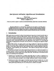
As in the Java source language, bytecode programs are organized in classes and methods. The JVM is a stack based abstract machine for bytecode programs. It comprises a heap, which stores objects, and a method call stack, which captures information about currently active methods in the form of frames. When the JVM invokes a method, it pushes a new frame onto the frame stack to store the method’s local data and its execution state. As Figure 1.1 illustrates, each frame contains its own program counter, operand stack, and register set. Bytecode programs specify the number of stack and register slots they use; this allows an implementation to allocate an activation record of the correct size for each method invocation. Bytecode instructions manipulate either the heap, the registers, or the operand stack. For example, the IAdd instruction removes the topmost two values (integers) from the operand stack, adds them, and pushes the result back onto the stack. In the example in Figure 1.1, the JVM would execute the Getfield F A instruction, removing the reference to the object from the stack, and putting the value (Addr 9 ) of the field F of the referenced object (at Addr 8 ) on top. Apart from the operand stack, the JVM uses registers to store the working data and arguments of the method. The first register (number 0 ) is reserved for the this pointer of the method. The next p registers are reserved for the p parameters of the method, and the rest is usually dedicated to local variables declared inside the method.
4
1.4 The Bytecode Verifier
Program (classes, methods, constants)
Frame Stack
Class A extends Object Field A F
Class A, Method void m() registers
stack [Addr 8]
[Addr 8, Addr 9]
pc 5
Class ..., Method ... stack
registers
...
...
Method void m(): … Load 0 Store 1 Load 0 Getfield F A Goto -3 ...
2 3 4 5 6
pc
Heap (objects, fields, arrays)
Class ..., Method ... stack
registers
...
...
pc
... Addr 7: ... Addr 8: Object of Class B, A.F = Addr 9 Addr 9: Object of Class A, A.F = Null Addr 10: ... ...
Figure 1.1: The JVM. The heap stores dynamically created objects, while the operand stack and registers only contain references to objects. Exception handlers for each method are specified in a table of tuples (s,e,h,C ). If an exception of class E is raised by an instruction in the asymmetric interval [s,e) and E is a subclass of C, the table entry is said to match the exception. The JVM looks for the first table entry that matches E, and transfers control to the instruction at h, the exception handler. The instructions in the JVM are typed. This means that, for example, the IAdd instruction only works on integers, not addresses. Similarly, a Getfield F A instruction that accesses the field F of an object on the heap only works on references of the correct class (any subclass of A). Using the Getfield or Invoke instructions on an integer would be an attempt to forge an object reference.
1.4
The Bytecode Verifier
The JVM relies on the following assumptions for executing bytecode: Correct types All bytecode instructions are provided with arguments of the type they
5
Chapter 1
Introduction
instruction -
Load 0 Store 1 Load 0 Getfield F A Goto −3
stack Some Some Some Some Some
registers
( [], [Class B , ( [Class A], [Class B , ( [], [Class B , ( [Class B ], [Class B , ( [Class A], [Class B ,
Integer ] Err ] Class A] Class A] Class A]
) ) ) ) )
Figure 1.2: Example of a method welltyping. expect on operand stack, registers, and heap. No overflow and underflow No instruction tries to retrieve a value from an empty stack, no instruction tries to put more elements on the stack than statically specified in the method, and no instruction accesses more registers than statically specified in the method. Code containment The program counter never leaves the code array of the method. Specifically, it must not fall off the end of the method’s code or branch into the middle of an instruction encoding. Initialized registers All registers apart from the this pointer and the method parameters must be written to before they are first read. This corresponds to the definite assignment requirement for local variables on the source level. Initialized objects Before fields or methods of an object can be accessed, its constructor must be called. Each constructor in turn must first call the superclass constructor before it accesses fields and methods of the object. It is the purpose of the bytecode verifier to ensure statically that these assumptions are met at any time. Bytecode verification is an abstract interpretation of bytecode methods: instead of values, we only consider their types. The BV can be viewed as a finite state machine working on state types. A state type characterizes a set of runtime states by giving type information for the operand stack and registers. For example, the first state type in Figure 1.2 ([],[Class B , Integer ]) characterizes all states whose stack is empty, whose register 0 contains a reference to an object of class B (or to a subclass of B ), and whose register 1 contains an integer. A method is called welltyped if we can assign a welltyping to each instruction. A state type (st,lt) is a welltyping for an instruction if it can be
6
1.5 Related Work executed safely on a state whose stack is typed according to st and whose registers are typed according to lt. In other words: the arguments of the instruction are provided in correct number, order and type. Let’s look at an example. Figure 1.2 shows the instructions on the left and the type of stack elements and registers on the right. The method type is the full right-hand side of the table, a state type is one line of it. The type information attached to an instruction characterizes the state before execution of that instruction. The Some before each of the entries means that it was possible to predict some type for each of the instructions. If one of the instructions had been unreachable, the type entry would have been None. We assume that class B is a subclass of A and that A has a field F of type A. Execution starts with an empty stack and the two registers holding a reference to an object of class B and an integer. The first instruction loads register 0, a reference to a B object, on the stack. The type information associated with the following instruction may puzzle at first sight: it says that a reference to an A object is on the stack, and that usage of register 1 may produce an error. This means the type information has become less precise but is still correct: a B object is also an A object and an integer is now classified as unusable (Err ). The reason for these more general types is that the predecessor of the Store instruction may have either been Load 0 or Goto −3. Since there exist different execution paths to reach Store, the type information of the two paths has to be merged. The type of the second register is either Integer or Class A, which are incompatible: the only common supertype is Err. Bytecode verification is the process of inferring the types on the right from the instruction sequence on the left and some initial condition, and of ensuring that each instruction receives arguments of the correct type. Type inference is the computation of a method type from an instruction sequence, type checking means checking that a given method type fits an instruction sequence. Figure 1.2 was an example for a welltyped method: we were able to find a welltyping. If we changed the third instruction from Load 0 to Store 0, the method would not be welltyped. The Store instruction would try to take an element from the empty stack and could therefore not be executed. We would also not be able to find any other method type that is a welltyping.
1.5
Related Work
This section provides an overview of the literature on bytecode verification and gives pointers to work related to this thesis. Most closely related are other formalizations of the JVM or the BV in theorem provers:
7
Chapter 1
Introduction
• Barthe et al. [5, 6] employ the Coq system [23] for proofs about the JavaCard [54] virtual machine and its BV. They formalize the full JavaCard bytecode language, but have only a simplified treatment of subroutines. In [2, 3, 4], they show how to increase automation in the process of specifying a defensive machine [22] (with safety checks), an aggressive machine (without safety checks), and an abstract machine (on the type level), together with their proofs of correspondence. • Bertot [10] also uses the Coq system to prove the correctness of a bytecode verifier based on the type system by Freund and Mitchell [27]. He focuses on object initialization only. • Posegga and Vogt [67] look at bytecode verification from a model checking perspective. They transform a given bytecode program into a finite state machine and check type safety, which they phrase in terms of temporal logic, by using an offthe-shelf model checker. Basin, Friedrich, and Gawkowski [7] use Isabelle/HOL, µJava, and the abstract BV framework, of which I present an extended version here, to prove the model checking approach correct. • The formalizations in this thesis are part of the work on the Java language of the Isabelle team in Munich, mainly in the projects Bali [1] and VerifiCard [89]. The specification of the BV is based on groundwork by Nipkow [58] and Pusch [68]. Nipkow, von Oheimb, and Schirmer [60, 62, 64, 65, 66, 76, 90, 91] have formalized the Java source language in Isabelle. Strecker [40, 85, 86] has proved correct a compiler for µJava from source to bytecode language in Isabelle, and has also shown that all welltyped programs of the source language are accepted by the bytecode verifier. Earlier, restricted forms of my formalization for standard and lightweight bytecode verification have appeared in [37, 38, 39]. The following projects use tool support to specify or implement bytecode verification: • Working towards a verified implementation in Specware, Qian, Goldberg and Coglio have specified and analyzed large portions of the bytecode verifier [18, 19]. Goldberg [29] rephrases and generalizes the overly concrete description of the BV given in the JVM specification [51] as an instance of a generic data flow framework. Qian [69] specifies the BV as a set of typing rules, a subset of which was proved correct formally by Pusch [68]. Qian [70] also proves the correctness of an algorithm for turning his type checking rules into a data flow analyzer. However, his algorithm is still quite abstract. • The Kimera project [80] treats bytecode verification in an empirical manner. Its aim is to check bytecode verifiers by automated testing.
8
1.5 Related Work • Casset et al. [12, 13, 14, 72] use the B method to specify a bytecode verifier for a defensive JavaCard VM, which they then refine into an executable program that provably satisfies the specification. They focus on the scalability of the B method for such proofs. Due to its commercial environment, the full specification itself does not seem to be publicly available. Hence, it is difficult to judge what exactly they have proved, and which parts of the bytecode language and its properties their formalization contains. The most recent article in the series, by Requet [72], sheds some light on this. Although they claim to handle a large subset of the JavaCard VM and over one hundred instructions, he writes [72, p. 288]: As the aim of this work was to verify the scalability of the approach, instructions that would drastically increase the complexity of the model have been left out. Especially, those instructions include the instructions used for subroutines, for method calls and for objects handling. • St¨ark et al. [81, 82, 83] use Java and the JVM as a case study for abstract state machines. They formalize the process from compilation of Java programs down to bytecode verification, and also provide an executable version in ASM Gofer [77]. Their main theorem says that the bytecode verifier accepts all bytecode programs the compiler generates from valid Java sources. Proofs, however, are by pen and paper. They argue that this theorem does not hold for the full Java language. Therefore they introduce a stronger constraint for definite assignment than the JVM specification. The type system presented in Chapter 5 of this thesis makes this restriction unnecessary. The following publications present type systems for the JVM; Hartel and Moreau [34] as well as Leroy [47, 50] provide a more detailed overview and discussion, Wildmoser [93] concentrates on articles related to bytecode subroutines. • Stata and Abadi [84] were the first to specify a type system for a subset of Java bytecode that supports subroutines. The typing rules they use are clearer and more precise than the JVM specification, but they accept fewer safe programs. • Freund and Mitchell [27, 28] develop typing rules for increasingly large subsets of the JVM, including exception handling, object initialization, and subroutines. Freund surveys the costs and benefits of subroutines [25], and reaches the conclusion that they should have been left out of the bytecode language. The final formalization [26] considers an instruction set comparable to the one presented here. The formalization, especially the treatment of subroutines, is more complex and more restrictive than the one in this thesis. The proof of type safety for object initialization in Chapter 4 is based on the one in [26].
9
Chapter 1
Introduction
• Leroy [47, 50] gives a very good overview on bytecode verification, and proposes a polyvariant data flow analysis in the bytecode verifier to solve the subroutine problem. He also addresses the problem of on-card bytecode verification for Java smart cards by program transformation combined with a simplified BV [48, 49]. • Coglio [15, 16] and, independently, Brisset [11] provide a simple solution to the subroutine problem in bytecode verification that is akin to model checking. Chapter 5 uses this scheme as basis for the formalization of subroutines in µJava. Together with Qian and Golberg, Coglio formally specifies dynamic class loading [17, 21, 71]. Coglio also gives an overview of the description of the bytecode verifier in the JVM specification [51] and suggests several improvements [20]. • Hagiya and Tozawa [33] use indirect types in rules similar to those of Stata and Abadi [84] to tackle subroutines. These indirect types are of the form last(x ), denoting the type register x held before the subroutine. This avoids the loss of precision type merges induce for unused registers. • O’Callahan [63] uses type variables and continuations to handle subroutines. Although his approach accepts a large portion of type safe programs—even recursive subroutines could be supported—it remains unclear whether it can be realized efficiently. • Rose [73, 74, 75] presents a lightweight bytecode verification scheme that works similar to Necula’s proof carrying code [56]: the program is annotated with typing information which is checked by a simplified on-card verifier. In Section 2.5, I formalize a more general version of this algorithm and prove it correct. • Laneve and Bigliardi [44, 45, 46] have implemented a bytecode verifier that checks proper handling of thread monitors. • Knoblock and Rehof [42, 43] show how to turn the type system into a lattice even if it contains interfaces. • Yelland [94] reduces bytecode verification to Haskell type inference.
1.6
Isabelle
This section gives a short and not so gentle introduction to Isabelle. It is by no means comprehensive, but it introduces the Isabelle/HOL notation that is used in this thesis. For a gentler, deeper, and eminently readable introduction, I recommend [61].
10
1.6 Isabelle Isabelle [35] is a generic, interactive theorem prover. It is generic in the sense that it can be instantiated with different object logics. The most widely used of these object logics is Isabelle/HOL, simply typed higher order logic. Formalizations are organized in an acyclic graph of theories, each containing a set of declarations, definitions, and theorems. For the most part, the notation is the same as in standard mathematics and functional programming. Function application is written in curried style as in functional programming, so f a is the function f applied to the argument a. The notation for set comprehension deviates from standard mathematics: {x . P x } is the set of all x for which P x holds. The common {y. ∃ x . f x = y ∧ P x }, in mathematics written as {f x | P x }, is abbreviated by {f x |x . P x } in Isabelle/HOL. The following, for instance, defines the image of a set A under a function f : f ‘ A ≡ {f x |x . x ∈ A} Function update is written f (x := y). The formal definition uses λ-abstraction and an if-then-else expression. f (x := y) ≡ λx 0. if x 0 = x then y else f x 0 The equivalence sign ≡ is used for definitions that are true abbreviations. Recursive definitions are formulated with simple equality =. New data types can be introduced with the datatype keyword, simple type abbreviations use types. Examples are: types nat-pair = nat × nat datatype α list = Nil | Cons α (α list) The first line declares nat-pair to be the Cartesian product of nat and nat (the type of natural numbers). The second line declares the polymorphic data type of lists. The type constructor list takes the type variable α as argument (written in prefix as α list). The declaration says that a list on type α is either Nil, or a Cons with an element of type α as head and a list on type α as tail. Isabelle provides special syntax for Nil and Cons: the empty list is [], and x #xs stands for Cons x xs. Isabelle/HOL has a rich library of list functions: xs!n is the n-th element of the list xs, the operator @ is append, the notation [1 ..n(] is the list of natural numbers from 1 to n−1, and xs [n:= x ] sets the n-th element of xs to x. Apart from these, I will use functions known from functional programming:
11
Chapter 1
Introduction size rev take drop zip map filter
:: :: :: :: :: :: ::
α list ⇒ nat α list ⇒ α list nat ⇒ α list ⇒ α list nat ⇒ α list ⇒ α list α list ⇒ β list ⇒ (α × β) list (α ⇒ β) ⇒ α list ⇒ β list (α ⇒ bool ) ⇒ α list ⇒ α list
The filter function has special syntax: [x ∈xs. P x ] is short for filter (λx . P x ) xs. There are also functions particular to Isabelle: set transforms a list into a set, list-all2 is an executable universal quantifier on a pair of lists, satisfying list-all2 P xs ys = ((∀ (x ,y) ∈ set (zip xs ys). P x y) ∧ size xs = size ys) HOL is a logic of total functions. For modeling partial functions, the option datatype is useful: datatype α option = None | Some α A function f :: α ⇒ β option then returns Some x for defined results x, and None if it is undefined for an argument value. A function f :: α ⇒ β option is also called a map from α to β. Function update for maps has special syntax: f (x 7→ y) is short for f (x := Some y). Isabelle/HOL also knows Hilbert’s classical choice operator. The term SOME x . P x returns some x that satisfies P. As all functions in HOL are total, it also returns a value if no such x exists. In this case, nothing is known about this value. The formal proofs in this thesis use the Isabelle/Isar proof language [59, 92]. Isabelle/Isar proofs are fully formal and machine checked, but contrary to the proof script style usually found in theorem provers, the resulting proofs are readable for humans. I will neither introduce nor define Isabelle/Isar formally here, but rather give an example that should explain how to read the Isabelle proofs in this thesis. lemma example: assumes pq: ∃ x . P x ∧ Q x shows (∃ x . P x ) ∧ (∃ x . Q x ) proof − from pq obtain y where p: P y and q: Q y by auto from p have ∃ x . P x .. moreover from q have ∃ x . Q x ..
12
1.6 Isabelle ultimately show ?thesis .. qed
The example above is formulated in an especially verbose way to demonstrate as many language constructs as possible. The first three lines say that the proposition to be proved is (∃ x . P x ∧ Q x ) −→ (∃ x . P x ) ∧ (∃ x . Q x ). The resulting lemma is stored under the name example. Proofs in Isar can either be compound (proof . . . qed), or simple one-liners (by . . .). Intermediate, named facts in a proof can be established with the have and obtain commands. The proof above begins with the technically complex, but conceptually simple obtain command: from the assumption pq, we can get a witness y such that P y and Q y holds. The proof uses the auto proof method to show that this is actually true. From these two facts we can then conclude that both ∃ x . P x and ∃ x . Q x are true. The abbreviation .. indicates a trivial proof that only needs the application of one single rule. The moreover command is used to collect facts (here provided by have), while ultimately makes the collected facts available for another subproof. Below, on the left hand side is a proof fragment with moreover, and on the right side an equivalent one without. have P 1 . . . moreover have P 2 . . . moreover have P 3 . . . ultimately have P 4 . . .
have fact1: P 1 . . . have fact2: P 2 . . . have fact3: P 3 . . . from fact1 fact2 fact3 have P 4 . . .
The last command in the proof body (show ?thesis) solves the pending goal with a trivial one-rule proof. The term abbreviation ?thesis refers to the stated goal in the current proof block. In this case, ?thesis is (∃ x . P x ) ∧ (∃ x . Q x ). Term bindings like these can also be used in a pattern matching style: the fragment f (x +1 ) = y (is f ?z = -) binds ?z to x +1. Another concept of Isabelle that I will use extensively in this thesis is that of locales. A locale in Isabelle is a collection of constants, assumptions, and definitions. It is a useful tool for structuring theorems in a large development, because it defines a common context for a group of theorems. An example is: locale A = fixes xs :: α list assumes p: P xs defines g ≡ λf . map f xs
locale B = A + fixes ys :: α list assumes q: Q xs ys
13
Chapter 1
Introduction
The locale A above fixes a constant xs (a list of type α) for which P xs holds. It also defines an abbreviation g for map applied to xs. The locale B extends the context that A has built up by another constant ys, for which it assumes Q xs ys. The current version of Isabelle only allows proper abbreviations (using defines) in locales, no recursive function definitions (using, for instance, multiple equations). With a small trick1 , it is still possible to use recursive functions as if they were defined in the context of a locale. For the presentation in this thesis, I will therefore pretend that this technical limitation does not exist.
1.7
Overview
The formalization of bytecode verification for µJava rests on the abstract framework introduced in Chapter 2. It contains the lattice-theoretic concepts for the framework, an abstract definition of welltypings that builds on a semilattice and a transfer function, and two equally abstract definitions of executable algorithms for bytecode verification: the standard iterative data flow analysis and a lightweight bytecode verifier for resourceconstrained devices. The remaining chapters instantiate this framework step by step with increasingly expressive type systems. Chapter 3 contains a first simple type system for classes, objects, inheritance, virtual methods, and exception handling. As in the following chapters, the instantiation results in two executable bytecode verifiers for µJava: Kildall’s algorithm and the lightweight bytecode verifier. Chapter 3 also describes in detail the formalization of the µJVM and the proof of correctness for both bytecode verifiers. Chapter 4 extends the type system of Chapter 3 by constructors and object initialization. This feature of the bytecode verifier ensures that all objects are properly initialized before they are used. Chapter 5 in turn extends the formalization of Chapter 4 by bytecode subroutines. This entails a substantial change in the type system. It is the first formalization in a theorem prover of a type system for Java that contains bytecode subroutines together with object initialization and exception handling. Chapter 6 adds arrays to the language. Chapter 7 concludes with a summary and pointers to further work.
1
First define the recursive function outside the locale context, then define an abbreviation of this function inside the locale, and finally derive the defining equations in the locale as theorems.
14
2 An Abstract Framework
The formalizations of bytecode verification in this thesis are instances of the abstract typing framework in this chapter. The framework takes a semilattice and a transfer function as parameters and yields a description of welltypings, an executable, verified version of Kildall’s algorithm, and an executable, verified lightweight bytecode verifier for resource-constrained devices.
2.1
Introduction
This chapter presents an abstract framework for bytecode verification. It builds on the work by Nipkow [58]. Compared to [58] and further work by Nipkow and myself [39], it is more general and more flexible in that it can be instantiated with more type systems. Semilat
Err
Listn
Opt
Product
SetSemilat
Typing_Framework
Typing_Framework_err
SemilatAlg
LBVSpec
Kildall
LBVCorrect
LBVComplete
Figure 2.1: Abstract framework overview.
15
Chapter 2
An Abstract Framework
Figure 2.1 gives an overview of the Isabelle theories that the abstract framework comprises. Section 2.2 describes the lattice-theoretic concepts of the framework, the upper three levels of Figure 2.1. Section 2.3 brings the definition of welltypings (theory Typing-Framework ), constraints on the transfer function (theory SemilatAlg), and a refinement of the transfer function (theory Typing-Framework-Err ). This part is more general than [39, 58]. The last two sections present two algorithms for bytecode verification: Section 2.4 shows the formalization of Kildall’s algorithm, Section 2.5 the lightweight bytecode verifier. Both algorithms can be instantiated with different type systems, are executable, and verified in Isabelle/HOL.
2.2
Semilattices
This section introduces the formalization of the basic lattice-theoretic concepts required for data flow analysis and its application to the JVM. Since most of this already appeared in [39, 58], I here only reproduce the definitions and main properties without proof.
2.2.1
Partial Orders
Partial orders are formalized as binary predicates. Based on the type synonym α ord = α ⇒ α ⇒ bool and the notations x ≤r y = r x y and x
2.2.2
bottom :: α ord ⇒ α ⇒ bool bottom r ⊥ ≡ ∀ x . ⊥ ≤r x
Semilattices
Based on the supremum notation x tf y = f x y and the two type synonyms α binop = α ⇒ α ⇒ α and α sl = α set × α ord × α binop, the tuple (A,r ,f ) :: α sl is by
16
2.2 Semilattices definition a semilattice iff the predicate semilat :: α sl ⇒ bool holds: semilat (A,r ,f ) ≡ order r ∧ closed A f ∧ (∀ x y ∈ A. x ≤r x tf y) ∧ (∀ x y ∈ A. y ≤r x tf y) ∧ (∀ x y z ∈ A. x ≤r z ∧ y ≤r z −→ x tf y ≤r z )
where closed A f ≡ ∀ x y ∈ A. x tf y ∈ A. Data flow analysis is usually phrased in terms of infimum semilattices. Here, a supremum semilattice fits better with the intended application, where the ordering is the subtype relation and the join of two types is the least common supertype (if it exists). The following Isabelle locale is used below. locale semilat = fixes A :: α set and r :: α ord and f :: α binop assumes semilat: semilat(A,r ,f ) The next sections look at a few data types and the corresponding semilattices which are required for the construction of the µJVM bytecode verifier. The definition of those semilattices follows a pattern: they lift an existing semilattice to a new semilattice with more structure. They extend the carrier set and define two functionals le and sup that lift the ordering and supremum operation to the new semilattice. In order to avoid name clashes, Isabelle provides separate names spaces for each theory. Qualified names are of the form Theoryname.localname, and they apply to constant definitions and functions as well as type constructions. So Err .sup later on refers to the sup functional defined for the error type in Section 2.2.3.
2.2.3
The Error Type and Err-semilattices
Theory Err introduces an error element to model the situation where the supremum of two elements does not exist. It introduces both a data type and an equivalent construction on sets: datatype α err = Err | OK α
err A ≡ {Err } ∪ {OK a |a. a ∈ A}
An ordering r on α can be lifted to α err by making Err the top element: le r (OK x ) (OK y) le r Err le r Err (OK y)
= = =
x ≤r y True False
17
Chapter 2
An Abstract Framework
Lemma 2.1 If r is a partial order that satisfies the ascending chain condition, then le r also is a partial order that satisfies the ascending chain condition. The following lifting functional is frequently useful: lift2 :: (α ⇒ β ⇒ γ err ) ⇒ α err ⇒ β err ⇒ γ err lift2 f (OK x ) (OK y) = f x y lift2 f = Err
This leads to the notion of an err-semilattice. It is a variation of a semilattice with top element. Because the behaviour of the ordering and the supremum on the top element is fixed, it suffices to say how they behave on non-top elements. Thus we can represent a semilattice with top element Err compactly by a triple of type esl : α ebinop = α ⇒ α ⇒ α err
α esl = α set × α ord × α ebinop
Conversion between the types sl and esl is easy: esl :: α sl ⇒ α esl esl (A,r ,f ) = (A, r , λx y. OK (f x y))
sl :: α esl ⇒ α err sl sl (A,r ,f ) = (err A, le r , lift2 f )
A tuple L :: α esl is by definition an err-semilattice iff sl L is a semilattice. Conversely, we get Lemma 2.2. Lemma 2.2 esl L is an err-semilattice if L is a semilattice. The supremum operation of sl (esl L) is useful on its own: sup f = lift2 (λx y. OK (x tf y))
2.2.4
The Option Type
Theory Opt introduces the new type option and the set opt as duals to type err and set err, datatype α option = None | Some α
opt A ≡ {None} ∪ {Some a |a. a ∈ A}
an ordering that makes None the bottom element, and a corresponding supremum operation:
18
2.2 Semilattices le r (Some x ) (Some y) = x ≤r y le r None = True le r (Some x ) None = False
sup f (Some x ) (Some y) = Some(f x y) sup f None z =z sup f z None =z
Lemma 2.3 sl (A,r ,f ) = (opt A, le r , sup f ) maps semilattices to semilattices. Lemma 2.4 le preserves the ascending chain condition.
2.2.5
Products
Theory Product provides what is known as the coalesced product, where the top elements of both components are identified. In terms of err-semilattices, this is: esl :: α esl ⇒ β esl ⇒ (α × β) esl esl (A,r A ,f A ) (B ,r B ,f B ) = (A × B , le r A r B , sup f A f B ) le :: α ord ⇒ β ord ⇒ (α × β) ord le r A r B = λ(a 1 ,b 1 )(a 2 ,b 2 ). a 1 ≤rA a 2 ∧ b 1 ≤rB b 2 sup :: α ebinop ⇒ β ebinop ⇒ (α × β) ebinop sup f g = λ(a 1 ,b 1 )(a 2 ,b 2 ). Err .sup (λx y.(x ,y)) (a 1 tf a 2 ) (b 1 tg b 2 )
Note that × is used both on the type and the set level. Lemma 2.5 If both L1 and L2 are err-semilattices, so is esl L1 L2 , Lemma 2.6 If both r A and r B satisfy the ascending chain condition, so does le r A r B .
2.2.6
Lists of Fixed Length
Theory Listn provides the concept of lists of a given length over a given set. In HOL, this is formalized as a set rather than a type: list n A = {xs. size xs = n ∧ set xs ⊆ A} This set can be turned into a semilattice in a componentwise manner, essentially viewing it as an n-fold Cartesian product: sl :: nat ⇒ α sl ⇒ α list sl sl n (A,r ,f ) = (list n A, le r , map2 f )
le :: α ord ⇒ α list ord le r = list-all2 (λx y. x ≤r y)
19
Chapter 2
An Abstract Framework
where map2 :: (α ⇒ β ⇒ γ) ⇒ α list ⇒ β list ⇒ γ list and list-all2 :: (α ⇒ β ⇒ bool ) ⇒ α list ⇒ β list ⇒ bool are the obvious functions. Below, I use the notation xs ≤[r ] ys for xs ≤(l e r ) ys. Lemma 2.7 If L is a semilattice, so is sl n L. Lemma 2.8 If r is a partial order and satisfies the ascending chain condition, then le r also is a partial order that satisfies the ascending chain condition. In case we want to combine lists of different lengths, or if the supremum on the elements of the list may return Err (not to be confused with Err .sup the sup functional defined in Theory Err, Section 2.2.3), the following function is useful: sup :: (α ⇒ β ⇒ γ err ) ⇒ α list ⇒ β list ⇒ γ list err sup f xs ys = if size xs = size ys then coalesce (map2 f xs ys) else Err coalesce [] = OK [] coalesce (e#es) = Err .sup (λx xs. x #xs) e (coalesce es)
This corresponds to the coalesced product. Below, we also need the structure of all lists up to a specific length: uptoesl :: nat ⇒ α esl ⇒ α list esl S uptoesl n (A,r ,f ) = ( i ≤ n listn i A, le r , sup f )
Lemma 2.9 If L is an err-semilattice, so is uptoesl n L.
2.2.7
Sets
Theory SetSemilat shows that finite sets form a semilattice. The order is the usual subset relation ⊆, and the supremum is union ∪. It is easy to see that (Pow A, ⊆, ∪) is a semilattice (where Pow A is the power set of A). Unfortunately, the subset relation allows infinitely ascending chains, and hence violates the ascending chain condition, which is needed below. Even if we only take the finite subsets in Pow A, there may be infinitely ascending chains. For example, consider the following sets of natural numbers: {} ⊂ {0 } ⊂ {0 ,1 } ⊂ {0 ,1 ,2 } ⊂ . . .
20
2.3 Stability Each of these is finite, but the chain continues ad infinitum. If the carrier set A itself is finite, however, ⊆ does satisfy the ascending chain condition on Pow A: Lemma 2.10 If A is finite, (Pow A, ⊆, ∪) is a semilattice and ⊆ satisfies the ascending chain condition on Pow A.
2.3
Stability
This section describes welltypings abstractly. The framework presented here is an extended, more general version of [39, 58]. I begin with the notion of welltyping in Section 2.3.1, continue with restrictions on the transfer function in Section 2.3.2, and conclude with a refinement of the transfer function in Section 2.3.3.
2.3.1
Welltypings
In this abstract setting, there is no need yet to talk about the instruction sequences themselves. They will be hidden inside a function that characterizes their behaviour. This function and a semilattice form the parameters of the model. Data flow analysis and type systems are based on an abstract view of the semantics of a program in terms of types instead of values. At this level, programs are sequences of instructions, and the semantics can be characterized by a function step :: nat ⇒ σ ⇒ (nat × σ) list. It is the abstract execution function: step p s provides the results of executing the instruction at p, starting in state s, together with the positions to which these results are propagated. Contrary to the usual concept of transfer function or flow function in the literature, step p not only provides the result, but also the structure of the data flow graph at position p. This is best explained by example. Figure 2.2 depicts the information we get when step 3 s 3 returns the list [(1 ,t 1 ),(4 ,t 4 )]: executing the instruction at position 3 with state type s 3 may lead to position 1 in the graph with result t 1 , or to position 4 with result t 4 . Note that the length of the list and the target instructions do not only depend on the source position p in the graph, but also on the value of s. It is possible (and for the Ret instruction necessary) that the structure of the data flow graph dynamically changes in
21
Chapter 2
An Abstract Framework t1
s0
s 1
s3
s4 t4
Figure 2.2: Data flow graph for step 3 s3 = [(1,t1 ),(4,t4 )]. the iteration process of the analysis. It may not change freely, however. Section 2.3.2 will introduce certain constraints on the step function that the analysis needs in order to succeed. The two definitions below are in the following context. locale stability = semilat + fixes step :: nat ⇒ σ ⇒ (nat × σ) list Data flow analysis is concerned with solving data flow equations, which are systems of equations involving the flow functions over a semilattice. In this case, step is the flow function and σ the semilattice. Instead of an explicit formalization of the data flow equation, it suffices to consider certain prefixed points. To that end I define what it means that a method type ϕ :: σ list is stable at p: stable ϕ p ≡ ∀ (q,s 0)∈set(step p (ϕ!p)). s 0 ≤r ϕ!q Stability induces the notion of a method type ϕ being a welltyping w.r.t. step: wt-step ϕ ≡ ∀ p ∧ stable ϕ p > is assumed to be a special element in the state space (the top element of the ordering). It indicates a type error. An instruction sequence is welltyped, if there is a welltyping ϕ such that wt-step ϕ.
2.3.2
Constraints on the Transfer Function
This section defines constraints on the transfer functions that the algorithms in Section 2.4 and 2.5 need to succeed. The transfer function step is called monotone up to n iff the following holds:
22
2.3 Stability mono step n r A ≡ ∀ p and a bottom element ⊥ in the semilattice. In Isabelle, this context is the following: locale lbv = semilat + fixes T :: σ (>) and B :: σ (⊥) fixes step :: nat ⇒ σ ⇒ (nat × σ) list assumes top: top r > and T-A: > ∈ A assumes bot: bottom r ⊥ and B-A: ⊥ ∈ A The top layer of the algorithm wtl is a single sweep through the instruction list that stops if any step returns the error element >.2 wtl :: α list ⇒ σ cert ⇒ nat ⇒ σ ⇒ σ wtl [] cps =s wtl (i #is) c p s = let s 0 = wtc c p s in if s 0=> ∨ s=> then > else wtl is c (p+1 ) s 0
The function wtl takes the instruction list, the certificate, a position in the instruction list, and an element of the semilattice. It yields an element of the semilattice. If this element is not >, the instructions are welltyped. In fact, as it is formulated here, the LBV will return exactly ⊥ for success and > for error. However, it is easier in the proofs not to require ⊥. The certificate is just a list of semilattice elements: types σ cert = σ list The LBV expects the certificate to contain the result state type at jump targets and the bottom element otherwise. The normal successor of an instruction at position p is p+1 ; all other successors are called the jump targets of the instruction. 2
The definition of wtl checks if s=>. If we assume that step is monotone (as it will be later), this check is unnecessary. With the check, however, we can prove soundness even without monotonicity.
30
2.5 Lightweight Bytecode Verification Each single step wtc of the LBV first looks at the certificate. If it contains ⊥, we proceed with the current state type s, if not, the current instruction is a jump target, which means the correct state type is more general than we expect, and we proceed with the information in the certificate instead. We also check that the certificate does not change s arbitrarily: it may only increase s. wtc :: σ cert ⇒ nat ⇒ σ ⇒ σ wtc c p s ≡ if c!p = ⊥ then wti c p s else if s ≤r c!p then wti c p (c!p) else >
The check s ≤r c!p is what makes the LBV safe: wtc does not rely completely on the certificate. The certificate is only allowed to make the computed information less precise, it must not make s more specific or even change s to something completely unrelated. The computation step wti for single instructions executes the transfer function step at position p and state type s and merges the results for the normal successor (the p+1 edge), while checking that the result is compatible with the certificate at all other successors (the jump targets). If p+1 is not among the successors, the next instruction must be a jump target to be reachable at all, so we can take the value in the certificate as the result. wti :: σ cert ⇒ nat ⇒ σ ⇒ σ wti c p s ≡ merge c p (step p s) (c!(p+1 )) merge :: σ cert ⇒ nat ⇒ (nat × σ) list ⇒ σ ⇒ σ merge c p [] x = x merge c p ((q,t)#ls) x = merge c p ls (if q=p+1 then t tf x else if t ≤r c!q then x else >)
The executable version of merge above is hard to reason about. If x is in A and snd ‘ set ss ⊆ A, the following equality holds: merge c p ss x = F if ∀ (q,t) ∈ set ss. q6=p+1 −→ t ≤r c!q then (map snd [(q,t) ∈ ss. q=p+1 ]) f x else > F
The (map . . .) f x expression is the start element x (the certificate at p+1 ) plus the sum over all (normal) successor state types (those (q,t) where q=p+1 ). Figure 2.4 demonstrates the merge function in an example. For the parameter values p=3, ss=[(4 ,t 1 ),(1 ,t 2 ),(4 ,t 3 )], and x =c!4, merge checks that t 2 ≤r c!1 and returns c!4 tf t 1 tf t 3 as the result (assuming the check was successful). If the instruction at position 4 is not a jump target (the regular case), the certificate will contain bottom, c!4 =⊥, and we get the desired t 1 tf t 3 . If the instruction is a jump
31
Chapter 2
An Abstract Framework
_r c!1 t2 < 1
t3
4
3 t1
method type c!4 certificate
c!1
c!4
Figure 2.4: The merge function with p=3, ss = [(4, t1 ), (1, t2 ), (4, t3 )], and x =c!4. target, however, the certificate should contain a value with t 1 ≤r c!4 and t 3 ≤r c!4 , so we get c!4 as result. Note that this does not make the safety check in wtc obsolete; quite to the contrary: we used the check (t 1 ≤r c!4 and t 3 ≤r c!4 ) to come to the result c!4.3 To demonstrate all possible cases, the example above is unrealistically complicated. In practice, step will most often return one element only (with q=p+1 ) and rarely a jump or a list with more than one successor (in the µJVM, this is only the case for conditional jumps, exception handlers, and the subroutine return instruction Ret). Although the algorithm above is directly executable in ML (using Isabelle’s code generator [9]), real implementations for embedded devices would optimize for the usual case of very short step lists.
2.5.3
Soundness
Since the LBV relies on outside information—the certificate—the immediate question is if this is a safe thing to do. The short answer is: yes. If the LBV accepts a piece of code as welltyped, the traditional bytecode verifier accepts it, too, regardless of what certificate was used. This specifically includes the case where the certificate or the program was tampered with. What happens in reality is that in such a case the LBV either rejects the program as not welltyped, or, if it does accept, the program is indeed welltyped and the tampering did no harm. The soundness theorem uses the notion of welltyping from Section 2.3.1. Theorem 2.2 If step is bounded by size ins and preserves A up to size ins, if the certificate is wellformed up to size ins, and if s 0 ∈ A, then wtl ins c 0 s 0 6= > −→ (∃ ϕ. wt-step ϕ) 3
One could change the ≤r in wtc to =, but the correspondence to stability is more visible this way.
32
2.5 Lightweight Bytecode Verification lemma (in lbv-sound ) phi-not-top: assumes wtl : wtl ins c 0 s 0 6= > and p: p < size ins shows ϕ!p 6= > proof (cases c!p = ⊥) case False with p have ϕ!p = c!p .. also from cert p have . . . 6= > .. finally show ?thesis . next case True with p have ϕ!p = wtl (take p ins) c 0 s 0 .. also from wtl have . . . 6= > .. finally show ?thesis . qed
Figure 2.5: Proof of Lemma phi-not-top in Isabelle/Isar. A certificate c is wellformed up to n if c!n=⊥, and if for all positions i below n, c!i is an element of A other than the top element. wf-cert c n ≡ (∀ i ) ∧ (c!n = ⊥) The proof of Theorem 2.2 constructs a witness ϕ for wt-step ϕ. Welltypedness requires that ϕ is stable and not equal to > at all positions p < size ϕ. Such a ϕ is easy to find: the LBV reconstructs ϕ during the sweep through the instructions. If available, we take the information in the certificate, for the rest we observe what state types the LBV calculates. Locale lbv-sound defines the context of the soundness proof, and with it, the witness ϕ. locale lbv-sound = lbv + fixes s 0 :: σ and c :: σ cert and ins :: α list and phi :: σ list (ϕ) assumes s0 : s 0 ∈ A and bounded : bounded step (size ins) assumes cert: wf-cert c (size ins) and pres: preserves step (size ins) A defines phi-def : ϕ ≡ map (λp. if c!p = ⊥ then wtl (take p ins) c 0 s 0 else c!p) [0 ..size ins(]
The first part of wt-step, ϕ!p 6= >, is easy. The proof is by case distinction on the certificate: if there is an entry in p, then ϕ will have the same entry, and it cannot be > since the certificate is wellformed. If there is no entry, then ϕ is the intermediate state type calculated by wtl up to p. This cannot be > either, because otherwise wtl would not have succeeded at all. Figure 2.5 shows this proof in Isabelle/Isar.
33
Chapter 2
An Abstract Framework
lemma (in lbv-sound ) wtl-stable: assumes wtl : wtl ins c 0 s 0 6= > and p: p < size ins shows stable ϕ p proof (unfold stable-def , clarify) fix q s 0 assume step: (q,s 0) ∈ set (step p (ϕ!p)) (is - ∈ set (?step p)) from bounded p step have q: q < size ins by (rule boundedD) have tkp: wtl (take p ins) c 0 s 0 6= > (is ?s1 6= -) .. have s 2 : wtl (take (p+1 ) ins) c 0 s 0 6= > (is ?s2 6= -).. from wtl p have wt-s 1 : wtc c p ?s1 6= > .. have c-Some: ∀ p t. p < size ins −→ c!p 6= ⊥ −→ ϕ!p = c!p by (simp add : phi-def ) have c-None: c!p = ⊥ =⇒ ϕ!p = ?s1 .. from wt-s 1 p c-None c-Some have inst: wtc c p ?s1 = wti c p (ϕ!p) by (simp add : wtc split: split-if-asm) have ?s1 ∈ A by (rule wtl-pres) with p c-Some cert c-None have ϕ!p ∈ A by (cases c!p = ⊥) (auto dest: cert-okD1 ) with p pres have step-in-A: snd‘set (?step p) ⊆ A by (auto dest: pres-typeD2 ) show s 0 ≤r ϕ!q proof (cases q = p+1 ) case True — q is a normal successor with q cert have cert-in-A: c!(p+1 ) ∈ A by (auto dest: cert-okD1 ) from True q have p1 : p+1 < size ins by simp with tkp have ?s2 = wtc c p ?s1 by − (rule wtl-Suc) with inst have merge: ?s2 = merge c p (?step p) (c!(p+1 )) by (simp add : wti ) also from s 2 merge have . . . 6= > (is ?merge 6= -) by simp with cert-in-A step-in-A F have ?merge = (map snd [(q,t)∈?step p. q=p+1 ] f (c!(p+1 ))) .. finally have s 0 ≤r ?s2 using step-in-A cert-in-A True step by (auto intro: pp-ub1 0) also from wtl p1 have ?s2 ≤r ϕ!(p+1 ) by (rule wtl-suc-pc) also note True [symmetric] finally show ?thesis by simp next case False — q is a jump target from wt-s 1 inst have merge c p (?step p) (c!(p+1 )) 6= > by (simp add : wti ) with step-in-A have ∀ (q,s 0)∈set (?step p). q6=p+1 −→ s 0 ≤r c!q by − rule with step False have ok : s 0 ≤r c!q by blast moreover from ok have c!q = ⊥ =⇒ s 0 = ⊥ by simp moreover from c-Some q have c!q 6= ⊥ =⇒ ϕ!q = c!q by auto ultimately show ?thesis by (cases c!q = ⊥) auto qed qed
Figure 2.6: Proof of Lemma wtl-stable in Isabelle/Isar.
34
2.5 Lightweight Bytecode Verification The second part of wt-step, stability, is more involved. Let’s take a look at Lemma wtl-stable in Figure 2.6: we may assume p < size ins and (q,s 0) ∈ set (step p (ϕ!p)) for some fixed p, q, and s 0. We have to show that ϕ is stable at p, i.e., that s 0 ≤r ϕ!q. The proof begins with a series of observations that concern wellformedness conditions and the nature of ϕ!q: since step is bounded, q is below size ins; wtl executed up to p and p+1 is not >, which means that all checks in the computation up to p+1 have been successful; ϕ is either wtl up to p or the same as the certificate c!p; all state types in the proof are in the carrier set (because step preserves A). After these observations, the proof proceeds with a case distinction whether q is a normal successor or a jump target. If q is a normal successor, q=p+1, we can conclude that the computation step wtc at F position p results in s 2 = map snd [(q,t)∈step p (ϕ!p). q=p+1 ] f (c!q). By definition of ϕ!q, we know s 2 ≤r ϕ!q (actually, we know s 2 = ϕ!q, since c!q is an element of the sum, but ≤r is all we need). Since s 0 is also an element of the sum in the merge expression, it follows that s 0 is smaller than the sum and therefore also smaller than ϕ!q. This concludes the normal successor case. If q is a jump target of the instruction at p, i.e., q6=p+1, then we have on the one hand that ϕ!q = c!q and on the other hand that the computation step wtc at p must have checked that s 0 ≤r c!q. The computation step was successful, so we again have s 0 ≤r ϕ!q. For the instantiation of the LBV in Chapters 3 to 6, a slightly more precise version of Theorem 2.2 is more convenient. Theorem 2.3 In the lbv-sound context, the following holds: wtl ins c 0 s 0 6= > ∧ ins 6= [] −→ (∃ ϕ ∈ list (size ins) A. wt-step ϕ ∧ s 0 ≤r ϕ!0 ) The proof just repeats the reasoning of lemma wtl-stable for q=0. The additional premise ins 6= [] is there because we need q < size ins.
2.5.4
Completeness
The soundness theorem ensures that the LBV is safe. The completeness theorem in this sections says that the LBV is also useful: if an instruction sequence is welltyped, it is possible to create a certificate such that the LBV succeeds. The certificate c is easy to construct: we take a welltyping, computed off-card by a standard BV or by the compiler as in [40, 86], and remove all entries that are not jump
35
Chapter 2
An Abstract Framework
targets. For the certificate to be wellformed (in the sense of Section 2.5.3), we append ⊥ as the last element. The completeness theorem, then, is the following: Theorem 2.4 If c is constructed as above, step is monotone up to size ϕ, preserves A up to size ϕ, and is bounded by size ϕ, if set ϕ ⊆ A, s 0 ∈ A, ⊥ = 6 > and size ins = size ϕ, then wt-step ϕ ∧ s 0 ≤r ϕ!0 −→ wtl ins c 0 s 0 6= > In addition to the conditions of the soundness theorem, we now need step to be monotone, the size of ϕ to coincide with the instruction sequence (otherwise it might cover only a part of ins), and ⊥ = 6 >. The latter is required for the simple reason that we need to be able to distinguish success ⊥ from error > in the result of wtl. The premise s 0 ≤r ϕ!0 is reminiscent of the start condition the JVM bytecode verifier places on the first instruction (see for example Section 3.3.3). It plays a similar role here: it ensures a correct start state type. In Isabelle, the proof context for completeness is the following. Note that ϕ!p = 6 > is part of the wt-step premise in Theorem 2.4, so the phi assumption collapses to set ϕ ⊆ A there. locale lbv-complete = lbv + fixes phi :: σ list (ϕ) and c :: σ cert assumes mono: mono r step (size ϕ) A and pres: preserves step (size ϕ) A assumes phi : ∀ p < size ϕ. ϕ!p ∈ A ∧ ϕ!p 6= > and bounded : bounded step (size ϕ) assumes B-neq-T : ⊥ = 6 > defines cert-def : c ≡ map (λp. if is-target p then ϕ!p else ⊥) [0 ..length ϕ(] @ [⊥] The function is-target determines whether an instruction at position q is a jump target. If q is a jump target, there must be a predecessor p such that q is a successor, but not a normal successor of p. is-target :: nat ⇒ bool is-target q ≡ ∃ p t. q 6= p+1 ∧ p < size ϕ ∧ (q,t) ∈ set (step p (ϕ!p))
In the following, I will sketch the proof of Theorem 2.4. It builds on three important lemmas. Lemma 2.17 (stable-wtc) In the lbv-complete context, if p < size ϕ, then stable ϕ p −→ wtc c p (ϕ!p) 6= >
36
2.5 Lightweight Bytecode Verification
lemma (in lbv-complete) lbv-complete-lemma: assumes V wt-step: wt-step ϕ shows p s. p+size ls = size ϕ =⇒ s ≤r ϕ!p =⇒ s ∈ A =⇒ s6=> =⇒ wtl ls c p s 6= > proof (induct ls) fix p s assume s6=> thus wtl [] c p s 6= > by simp next fix p s i ls V assume p s. p+size ls=size ϕ =⇒ s ≤r ϕ!p =⇒ s ∈ A =⇒ s6=> =⇒ wtl ls c p s 6= > moreover assume p-l : p + size (i #ls) = size ϕ hence suc-p-l : Suc p + size ls = size ϕ by simp ultimately V have IH : s. s ≤r ϕ!Suc p =⇒ s ∈ A =⇒ s 6= > =⇒ wtl ls c (Suc p) s 6= > . from p-l obtain p: p < size ϕ by simp with wt-step have stable: stable ϕ p by (simp add : wt-step-def ) hence wt-phi : wtc c p (ϕ!p) 6= > by (rule stable-wtc) from phi p have phi-p: ϕ!p ∈ A by simp moreover assume s: s ∈ A and s-phi : s ≤r ϕ!p ultimately have wt-s-phi : wtc c p s ≤r wtc c p (ϕ!p) by − (rule wtc-mono) with wt-phi have wt-s: wtc c p s 6= > by simp moreover assume s: s 6= > ultimately have ls = [] =⇒ wtl (i #ls) c p s 6= > by simp moreover { assume ls 6= [] with p-l have suc-p: Suc p < size ϕ by (auto simp add : neq-Nil-conv ) with stable have wtc c p (ϕ!p) ≤r ϕ!Suc p by (rule wtc-less) with wt-s-phi have wtc c p s ≤r ϕ!Suc p by (rule trans-r ) moreover from cert suc-p have c!p ∈ A and c!(p+1 ) ∈ A by (auto simp add : cert-ok-def ) with pres have wtc c p s ∈ A by (rule wtc-pres) ultimately have wtl ls c (Suc p) (wtc c p s) 6= > using IH wt-s by blast with s wt-s have wtl (i #ls) c p s 6= > by simp } ultimately show wtl (i #ls) c p s 6= > by (cases ls) blast+ qed
Figure 2.7: Proof of wtl-complete-lemma in Isabelle/Isar.
37
Chapter 2
An Abstract Framework
Lemma 2.18 (wtc-less) In the lbv-complete context, if p+1 < size ϕ, then stable ϕ p −→ wtc c p (ϕ!p) ≤r ϕ!(p+1 ) Lemma 2.19 (wtc-mono) In the lbv-complete context, if p < size ϕ, s 1 ∈ A, and s 2 ∈ A, then s 2 ≤r s 1 −→ wtc c p s 2 ≤r wtc c p s 1 The first two lemmas, 2.17 and 2.18, are based on the observation that stable requires for all successors (q,t) in step p (ϕ!p) that t ≤r ϕ!q. The LBV focuses on those where q=p+1 for the computation, the rest is only checked (with the same condition). If all t with q=p+1 are smaller than ϕ!q, then also the sum of the t must be smaller than ϕ!q. The sum also contains the certificate c!q, but c!q is either ⊥ or equal to ϕ!q. In both cases we get c!q ≤r ϕ!q, and therefore wtc c p (ϕ!p) ≤r ϕ!q with q=p+1. Lemma 2.19 just lifts the monotonicity of step up to wtc. The proof of the main completeness theorem (Theorem 2.4) is then by induction on the instruction sequence. For the induction to go through, we have to strengthen the goal. Under the assumption wt-step ϕ, we show: ∀ p s. p+size ls = size ϕ ∧ s ≤r ϕ!p ∧ s ∈ A ∧ s6=> −→ wtl ls c p s 6= > Figure 2.7 contains the Isabelle/Isar proof for this lemma. The base case of the induction is as easy as it should be: from the assumption s6=> we immediately get wtl [] c p s 6= >. In the step case, there is a first instruction i and a rest list ls for which we have to show wtl (i #ls) c p s 6= >. The first steps in Figure 2.7 reduce the induction hyV pothesis to s. s ≤r ϕ!Suc p =⇒ s ∈ A =⇒ s 6= > =⇒ wtl ls c (Suc p) s 6= >. If we instantiate s with wtc c p s and can get our hands on the conclusion of the induction hypothesis wtl ls c (Suc p) (wtc c p s) 6= >, we have proved the goal, because wtl ls c (Suc p) (wtc c p s) is the same as wtl (i #ls) c p s provided wtc c p s 6= >. We may assume that s ≤r ϕ!p and (from wt-step ϕ) that stable ϕ p holds. To use the induction hypothesis, we have to show wtc c p s ≤r ϕ!(p+1 ), wtc c p s ∈ A, and wtc c p s 6= >. The proof in Figure 2.7 begins with the last of these premises. Using Lemma 2.17 (stable-wtc), we conclude wtc c p (ϕ!p) 6= > from stable ϕ p. With s ≤r ϕ!p we know by monotonicity (Lemma 2.19) of wtc that wtc c p s ≤r wtc c p (ϕ!p) and thus the desired wtc c p s 6= >. The next lines in Figure 2.7 handle the special case where ls = []. Here, we immediately have wtl (i #ls) c p = wtc c p s 6= >. The interesting case ls 6= [] gives us p+1 < size ϕ and we use Lemma 2.18 to get
38
2.5 Lightweight Bytecode Verification wtc c p (ϕ!p) ≤r ϕ!Suc p. Because we already know wtc c p s ≤r wtc c p (ϕ!p), we thereby also have the first premise of the induction hypothesis, wtc c p s ≤r ϕ!Suc p, by transitivity of ≤r . The remaining premise, wtc c p s ∈ A, follows from the fact that step is type preserving. With this, we can use the induction hypothesis and conclude the final goal wtl (i #ls) c p s 6= >. This concludes the proof of the induction lemma. Theorem 2.4 is a corollary of it.
2.5.5
Conclusion
Above, I have presented a framework for lightweight bytecode verification. It contains the lightweight bytecode verifier as an abstract and executable functional program that is sound and complete. Both properties are generic in the type system, proved with respect to the typing framework of Section 2.3.1. In this abstract setting, the main Isabelle/Isar proofs are small enough to be shown here. The specification of the lightweight bytecode verifier consists of only 37 lines of Isabelle definitions. The proofs of soundness and completeness including all related lemmas take up about 1000 lines of human-readable Isabelle/Isar text. The LBV-specific instantiation of the framework is about another 300 lines for each type system. The abstract setting of an arbitrary semilattice and the general step function allows the LBV to be used for all type systems I present in this thesis. Most notably, the structure of the data flow graph may again depend on the current state type, which enables the LBV to be used for the notorious bytecode subroutines [25] which are not supported by Sun’s KVM (they must be eliminated by expansion before verification). In comparison to my formalization, the original approach of Rose [74, 75] is less general and also a bit more complex. It is less general, because she cannot handle bytecode subroutines and because she formulates it for the JVM only.4 It is more complex because she does not distinguish type system from algorithm in the formalization, and because she includes a compression optimization for certificates: she only needs the certificate when a type merge really produces a different type than expected, which leads to a smaller type annotation. It does, however, not save space during the verification pass itself, since the state type at all jump targets has to be saved for later checks anyway. My completeness result includes the simpler and easier to implement notion that the certificate should contain all jump targets. This is also used in Sun’s KVM verifier. The soundness theorem states that the lightweight bytecode verifier accepts only type correct programs, and that it is safe to rely on outside information. The complete4
I have instantiated the LBV for the µJVM only, but in principle this algorithm is applicable wherever standard bytecode verification can be used.
39
Chapter 2
An Abstract Framework
ness theorem states that the lightweight bytecode verifier will accept the same welltyped programs as the traditional bytecode verifier. Both theorems combined tell us that lightweight bytecode verification is functionally completely equivalent to traditional bytecode verification. The functional implementation shows that the algorithm is linear in time and constant in space. All these results together enable a secure scheme for on-card verification with Java smartcards: programs are annotated with a certificate, produced by a traditional bytecode verifier or directly by the compiler off-card. On-card verification can then take place with the efficient and compact lightweight bytecode verifier as part of the card’s JVM. This scheme provides easy, seamless use for developers while maintaining all security properties from bytecode verification that we have become accustomed to. The major advantage over cryptographic methods is that no trust is needed at all in the certifying party and authenticity of the certificate.
40
3 Instantiating the Framework
In this chapter, I instantiate the abstract typing framework with a first, simple type system, show that this type system is sound, and derive two verified executable bytecode verifiers from the specification. I also describe in detail the JVM formalization and the structure of programs. Both the JVM and the BV will serve as basis for the extensions in Chapters 4 to 6.
3.1
Introduction
This chapter shows the formalization of the µJVM and its BV. The JVM formalization begins by defining types, values, programs, declarations, wellformedness conditions, and lookup functions. It proceeds with the memory and state model of the µJVM and finally shows the definition of the operational semantics. The semantics is split in two parts: an aggressive machine that executes programs without type and safety checks, and a defensive machine that includes those checks. The aggressive machine is closer to a real implementation, the defensive machine is useful to express type safety. It is shown that the two are equivalent if no type errors occur. The formalization of the BV is an instantiation of the framework in Chapter 2. It defines a suitable semilattice and transfer function and uses the theorems and definitions of the framework to derive a static description of welltypings together with two executable bytecode verifiers. With the definition of welltypings, it is then possible to show that all welltyped programs are type safe. The type system presented here is an extended, more modular version of [60]. It contains classes, inheritance, virtual methods, and exception handling. I keep it relatively simple to introduce the µJVM formalization, which is the basis for the proof of type safety, and to demonstrate a first instantiation of the abstract typing framework. The type safety proof uses the defensive machine for stating the theorem, and an invariant argument to show that execution remains safe. I describe the definition of the invariant as well as an exemplary case of the proof in Isabelle/Isar notation.
41
Chapter 3
Instantiating the Framework
Types & Programs
Type
Value
Decl
TypeRel
Framework
Semilat
Err
SystemClasses
Product
Opt
Listn
Typing_Framework
WellForm
State
JType
Conform
JVM
SemilatAlg
JVMType
JVMState
Typing_Framework_err
Kildall
LBV
JVMInstructions
JVMExecInstr
JVMExceptions
JVMExec
Effect
BVSpec
JVMDefensive
Correct
BVSpecTypeSafe
BVNoTypeError
EffectMono
Typing_Framework_JVM
LBVJVM
JVM
Concrete Type System & Bytecode Verifier
Figure 3.1: Instantiating the framework: overview. Figure 3.1 gives an overview of the Isabelle theories involved. The theory dependency graph in Figure 3.1 contains four clusters. The upper right corner shows the framework of Chapter 2 (the three LBV theories are merged into one to disentangle the picture). Section 3.2.1 will be concerned with the upper left corner, the machine independent part of µJava: types, declarations, and the structure of programs. The rest of Section 3.2 is dedicated to the definition of the µJVM and its operational semantics: the lower left of Figure 3.1. The remaining theories in Figure 3.1 contain the type system with the executable bytecode verifiers and its proof of soundness. Section 3.3 shows the type system and the bytecode verifiers, Section 3.4 the proof of type safety.
42
3.2 The µJava Virtual Machine
3.2
The µJava Virtual Machine
This section gives a detailed introduction to the µJava Virtual Machine. It contains the structure of µJava programs (Section 3.2.1), the state space of the µJVM (Section 3.2.2), and its operational semantics, first without (Section 3.2.3) and then with (Section 3.2.4) runtime type checks.
3.2.1
Structure
Declarations Since µJava formalizes both the source and the bytecode language, it distinguishes code from declarations in a special way: declarations are shared, code is a type variable that is instantiated later (with either bytecode language instructions or source language terms). This thesis will only be concerned with the bytecode level. The declaration structure of programs is the following in Isabelle: types
fdecl sig γ mdecl γ class γ cdecl γ prog
= = = = = =
vname × ty mname × ty list sig × ty × γ cname × fdecl list × γ mdecl list cname × γ class γ cdecl list
This is best read from bottom to top: a program γ prog with method bodies of type γ is a list of class declarations. A class declaration γ cdecl consists of the name of the class and the class itself. A class γ class is again a tuple: it consists of the name of the superclass, a list of field declarations, and a list of method declarations. A method declaration γ mdecl has a signature sig (name and parameter types of the method), a return type ty, and the body γ. A field declaration fdecl is a pair of field name and field type. Class names are based on a not further specified set of names cnam: datatype cname = Object | Xcpt xcpt | Cname cnam datatype xcpt = NullPointer | ClassCast | OutOfMemory The names of system exceptions and the name of class Object are predefined, all other classes have names out of cnam.
43
Chapter 3
Instantiating the Framework
For the bytecode level, the names of methods mname and the names of fields vname can be left unspecified like cnam. The HOL data type ty of basic types in µJava is the following: datatype ty = PrimT prim-ty | RefT ref-ty datatype prim-ty = Void | Boolean | Integer datatype ref-ty = NullT | ClassT cname The above means that a type ty is either a primitive type or a reference type. Primitive types can be the usual Void, Boolean, or Integer. Reference types are the null type (for the Null reference), and classes. For readability, µJava uses the following abbreviations, implemented as syntax translations in Isabelle: translations
* RefT NullT NT ) Class C * ) RefT (ClassT C )
A program Γ :: γ prog gives rise to a lookup function class that takes a program and a class name and returns the class if it is declared (and None otherwise). The function map-of :: (α × β) list ⇒ (α ⇒ β option) turns a list of pairs into a map. class :: γ prog ⇒ cname ⇒ γ class option class Γ ≡ map-of Γ
With this, we can determine if a class or a type is declared in a program: is-class :: γ prog ⇒ cname ⇒ bool is-class Γ C ≡ class Γ C 6= None is-type :: γ prog ⇒ ty ⇒ bool is-type Γ (PrimT t) = True is-type Γ (RefT t) = (case t of NullT ⇒ True | ClassT C ⇒ is-class Γ C )
Subtypes Each program Γ also induces a subtype ordering �. It builds on the direct subclass relation subcls Γ and satisfies: T NT Class C
44
� � �
T RefT T Class D
if (C ,D) ∈ (subcls Γ)∗
3.2 The µJava Virtual Machine The expression (C ,D) ∈ (subcls Γ)∗ means that C is a subclass of D in Γ. In Isabelle, subcls Γ is an inductive definition with the following sole introduction rule: [[class Γ C = Some (D,decl ); C 6= Object]] =⇒ (C ,D) ∈ subcls Γ For every class hierarchy, which means for every program, this subtype ordering may be a different one. In the Isabelle formalization, the ordering � therefore has Γ as an additional parameter. Here, I treat Γ as a global constant in most definitions. Wellformedness Like the Java Language Specification (JLS) [32], µJava imposes certain wellformedness constraints on programs. Wellformedness of fields and method headers is easy. A field declaration is wellformed if the field has a declared type, and a method header is wellformed if the return type and all parameter types are declared: wf-fdecl :: γ prog ⇒ fdecl ⇒ bool wf-fdecl Γ (fn,ft) ≡ is-type Γ ft wf-mhead :: γ prog ⇒ sig ⇒ ty ⇒ bool wf-mhead Γ (mn,ps) rt ≡ is-type Γ rt ∧ (∀ T ∈set ps. is-type Γ T )
Since method bodies γ are not instantiated yet, wellformedness of programs is parameterized with a function wf-mb that checks wellformedness of method bodies. For bytecode, this will later be the bytecode verifier. The type of wf-mb is types γ wf-mb = γ prog ⇒ cname ⇒ γ mdecl ⇒ bool This means the function wf-mb gets the program, the current class, and the current method declaration as input. With this information, it decides whether the method body is wellformed. A full method declaration is then wellformed if its header and its body are wellformed: wf-mdecl :: γ wf-mb ⇒ γ prog ⇒ cname ⇒ γ mdecl ⇒ bool wf-mdecl wf-mb Γ C (sig,rt,mb) ≡ wf-mhead Γ sig rt ∧ wf-mb Γ C (sig,rt,mb)
Wellformedness of class declarations is more involved.
45
Chapter 3
Instantiating the Framework
wf-cdecl :: γ wf-mb ⇒ γ prog ⇒ γ cdecl ⇒ bool wf-cdecl wf-mb Γ (C ,(D,fs,ms)) ≡ (∀ f ∈set fs. wf-fdecl Γ f ) ∧ unique fs ∧ (∀ m∈set ms. wf-mdecl wf-mb Γ C m) ∧ unique ms ∧ (C 6= Object −→ is-class Γ D ∧ (D,C ) ∈ / (subcls Γ)∗ ∧ 0 0 0 (∀ (sig,rt,b)∈set ms. ∀ D rt b . method (Γ,D) sig = Some(D 0,rt 0,b 0) −→ rt � rt 0))
The beginning of wf-cdecl is canonical: all field and method declarations must be wellformed, and each field and method should only be declared once (unique). The next line makes sure that all superclasses that are mentioned in declarations are actually declared in the program and that the subclass relation is acyclic. The last line is a bit less restrictive than the JLS: it requires that a method declared in class C has a return type smaller than the one of methods with the same signature, but defined in a superclass D of C. The JLS requires overriding methods to have the same return type as the overridden method. The method lookup function method will be defined formally below. Before that, I finish wellformedness: wf-syscls :: γ prog ⇒ bool wf-syscls Γ ≡ let cs = set Γ in Object ∈ fst‘cs ∧ (∀ x . Xcpt x ∈ fst‘cs) wf-prog :: γ wf-mb ⇒ γ prog ⇒ bool wf-prog wf-mb Γ ≡ unique Γ ∧ wf-syscls Γ ∧ (∀ c ∈ set Γ. wf-cdecl wf-mb Γ c)
The above says a program is wellformed (wf-prog) if each class is declared only once, if it is wellformed w.r.t. system classes, and if all class declarations are wellformed. It is wellformed w.r.t. system classes (wf-syscls) if it contains a declaration of the class Object and a declaration for each system exception. Finally, a program is called well structured (ws-prog Γ), if it wellformed without the method bodies: ws-prog Γ ≡ wf-prog (λΓ C mdecl . True) Γ
Lookup functions The method lookup function method and its analogue fields for fields are large and tedious recursive definitions in Isabelle. Slightly more readable are the following equations that hold if wf ((subcls Γ)−1 ) and class Γ C = Some (D,fs,ms):
46
3.2 The µJava Virtual Machine method :: γ prog × cname ⇒ (sig ⇒ (cname × ty × γ) option) method (Γ,C ) = (if C =Object then empty else method (Γ,D)) ++ map-of (map (λ(sig,rt,b). (sig,(C ,rt,b))) ms) fields :: γ prog × cname ⇒ ((vname × cname) × ty) list fields (Γ,C ) = map (λ(fn,ft). ((fn,C ),ft)) fs @ (if C =Object then [] else fields (Γ,D))
The method function looks up whether a method with signature sig exists in class C and program Γ. If it exists, it yields the name of the class the method is defined in (it could be a superclass of C ), the return type of the method, and the body of the method. If it does not exist, it yields None. The equation for method above first recurses into the superclass D and overwrites (using the ++ operator) the resulting map with the methods of the current class. Note that class Γ C = Some (D,fs,ms) ensures that ms is the list of method declarations in class C and that D is the superclass of C. The fields function is similar. For a class C in program Γ, it returns the list of all fields of this class (including those defined in superclasses). For each field, it returns its name, the name of the class it is defined in, and the field’s type. The equation above collects the fields of the current class and then recurses into the superclass D. Both functions walk up the class hierarchy. It is therefore necessary that the converse of subcls Γ is wellfounded (otherwise they would not terminate), hence the condition wf ((subcls Γ)−1 ). Note that whenever wf-prog mb Γ holds for any wellformedness condition mb of method bodies, wf ((subcls Γ)−1 ) must be true. Both functions are only specified if the class C in which they are supposed to look up a method or field does exist in Γ, hence the condition class Γ C = Some (D,fs,ms). The way both functions are formulated coincides with Java’s rules for inheritance and overriding. The fields function has a variant field that takes a program Γ, a class C, and a field name fn, and that returns Some (D,ft) if the field exists (where D is the class the field is defined in and ft the type of the field). If there is no field with name ft accessible in C, then field (Γ,C ) fn returns None. It is defined by: field :: γ prog × cname ⇒ (vname ⇒ (cname × ty) option) field ≡ map-of ◦ (map (λ((fn,C ),ft). (fn,(C ,ft)))) ◦ fields
Values The type val of values is defined by datatype val = Unit | Null | Bool bool | Intg int | Addr loc
47
Chapter 3
Instantiating the Framework
Unit is a (dummy) result value of void methods, Null the null reference. Bool and Intg are injections from the HOL types bool and int into val, similarly Addr from the type loc of locations. In the spirit of JavaCard, the type loc reserves space for preallocated system exception objects:1 datatype loc = XcptRef xcpt | Loc locs The type locs again remains unspecified.
3.2.2
State Space
The state space of the µJVM is modeled closely after the real JVM. The state consists of a heap, a stack of call frames, and a flag whether an exception was raised (and, if yes, a reference to the exception object). types jvm-state = val option × aheap × frame list The heap is simple: a partial function from locations to objects. types aheap = loc ⇒ obj option An object obj is a pair consisting of a class name (the class the object belongs to) and a mapping for the fields of the object (taking the name and defining class of a field, and yielding its value if such a field exists, None otherwise). types obj = cname × (vname × cname ⇒ val option) As in the real JVM, each method execution gets its own call frame, containing its own operand stack (a list of values), its own set of registers (also a list of values), and its own program counter. We also store the class and signature (name and parameter types) of the method and arrive at: types
1
frame = opstack × registers × cname × sig × nat opstack = val list registers = val list
Thus also avoiding the situation where there is no space left for a new OutOfMemory exception object.
48
3.2 The µJava Virtual Machine datatype instr = Load nat | Store nat | LitPush val | New cname | Getfield vname cname | Putfield vname cname | Checkcast cname | Invoke cname mname (ty list) | Return | Dup | Dup-x1 | IAdd | Goto int | Ifcmpeq int | Throw
load from register store into register push a literal (constant) create object on heap fetch field from object set field in object check if object is of class cname invoke instance method return from method duplicate top element duplicate top element and push 2 values down integer addition goto relative address branch if equal throw exception
Figure 3.2: The µJava bytecode instruction set.
3.2.3
Operational Semantics
This section defines the state transition relation of the µJVM. Figure 3.2 shows the instruction set. Method bodies are lists of such instructions together with the exception handler table and two numbers mxs and mxl . These are the maximum operand stack size and the number of local variables (not counting the this pointer and the parameters of the method, which are stored in the first 0 to n registers). So the type parameter γ for method bodies gets instantiated with nat × nat × instr list × ex-table; mdecl becomes the following: mdecl = sig × ty × nat × nat × instr list × ex-table Like in the JVM, the exception table is a list of tuples (start-pc, end-pc, handler-pc, C ): types ex-table = (nat × nat × nat × cname) list The asymmetric interval [start-pc, end-pc) denotes those instructions in the method body that correspond to the try block on the Java source level. The handler-pc points to the first instruction of the corresponding catch block. The code starting at handler-pc is the exception handler. An exception handler protects a program position pc iff pc ∈ [start-pc,end-pc). An exception table entry matches an exception e if the handler protects the current pc and if the class of e is a subclass of C. jvm
The state transition relation s −→ t is built on a function exec describing one-step execution:
49
Chapter 3 exec exec exec exec
Instantiating the Framework :: jvm-state ⇒ jvm-state option (xp, hp, []) = None (Some xp, hp, frs) = None (None, hp, f #frs) = let (stk ,reg,C ,sig,pc) = f ; ins = 5th (the (method (Γ,C ) sig)); i = ins ! pc in find-handler (exec-instr i hp stk reg C sig pc frs)
It says that execution halts if the call frame stack is empty or an unhandled exception has occurred. In all other cases, execution is defined: exec decomposes the top call frame, looks up the current method, retrieves the instruction list (the 5th element) of that method, delegates actual execution for single instructions to exec-instr, and finally sets the pc to the appropriate exception handler (with find-handler ) if an exception occurred. Exception handling in find-handler is the same as in the JVM specification: it looks up the exception table in the current method, and sets the program counter to the first handler that protects pc and that matches the exception class. If there is no such handler, the topmost call frame is popped, and the search continues recursively in the invoking frame. If this procedure does find an exception handler, it clears the operand stack and puts a reference to the exception on top. If it does not find an exception handler, the exception flag remains set and the machine halts. The state transition relation is the reflexive transitive closure of the defined part of exec: jvm
s −→ t = (s,t) ∈ {(s,t). exec s = Some t}∗ The definition of exec-instr in Figure 3.3 is large, but straightforward. One of the smaller definitions in exec-instr is the one for the IAdd instruction: exec-instr IAdd hp stk regs C 0 sig pc frs = let i 1 = the-Intg (hd stk ); i 2 = the-Intg (hd (tl stk )) in (None, hp, (Intg (i 1 +i 2 )#(tl (tl stk )), regs, C 0, sig, pc+1 )#frs)
It takes the top two values from the stack, converts them to HOL integers (using the equality the-Intg (Intg i ) = i ), adds them and puts the result back onto the stack. The program counter is incremented, the rest remains untouched. Most instructions in Figure 3.3 are of that simple form. Instructions with exceptions and heap access have larger definitions (due to case distinctions), but it should become clear that exec-instr follows the JVM specification closely.
50
3.2 The µJava Virtual Machine
exec-instr :: instr ⇒ aheap ⇒ opstack ⇒ registers ⇒ cname ⇒ sig ⇒ nat ⇒ frame list ⇒ jvm-state exec-instr (Load idx ) hp stk regs C 0 sig pc frs = (None, hp, ((regs ! idx ) # stk , regs, C 0, sig, pc+1 )#frs) exec-instr (Store idx ) hp stk regs C 0 sig pc frs = (None, hp, (tl stk , regs[idx :=hd stk ], C 0, sig, pc+1 )#frs) exec-instr (LitPush v ) hp stk regs C 0 sig pc frs = (None, hp, (v # stk , regs, C 0, sig, pc+1 )#frs) exec-instr (New C ) hp stk regs C 0 sig pc frs = let (a,xp 0) = new-Addr hp; hp 0 = if xp 0=None then hp(a7→blank Γ C ) else hp; pc 0 = if xp 0=None then pc+1 else pc in (xp 0, hp 0, ((Addr a) # stk , regs, C 0, sig, pc 0)#frs) exec-instr (Getfield F C ) hp stk regs C 0 sig pc frs = let r = hd stk ; xp 0 = raise-system-xcpt (r =Null ) NullPointer ; (c,fs) = the(hp(the-Addr r )); pc 0 = if xp 0=None then pc+1 else pc in (xp 0, hp, (the(fs(F ,C ))#(tl stk ), regs, C 0, sig, pc 0)#frs) exec-instr (Putfield F C ) hp stk regs C 0 sig pc frs = let (v ,r )= (hd stk , hd (tl stk )); xp 0 = raise-system-xcpt (r =Null ) NullPointer ; a = the-Addr r ; (c,fs) = the (hp a); hp 0 = if xp 0=None then hp(a7→(c,fs((F ,C )7→v ))) else hp; pc 0 = if xp 0=None then pc+1 else pc in (xp 0, hp 0, (tl (tl stk ), regs, C 0, sig, pc 0)#frs) exec-instr (Checkcast C ) hp stk regs C 0 sig pc frs = let r = hd stk ; xp 0 = raise-system-xcpt (¬ cast-ok Γ C hp r ) ClassCast; stk 0 = if xp 0=None then stk else tl stk ; pc 0 = if xp 0=None then pc+1 else pc in (xp 0, hp, (stk 0, regs, C 0, sig, pc 0)#frs)
Figure 3.3: Single step execution (part 1).
51
Chapter 3
Instantiating the Framework
exec-instr (Invoke C mn ps) hp stk regs C 0 sig pc frs = let n = size ps; args = take n stk ; r = stk !n; xp 0 = raise-system-xcpt (r =Null ) NullPointer ; dt = fst(the(hp(the-Addr r ))); (dc,-,-,mxl ,-)= the (method (Γ,dt) (mn,ps)); frs 0 = if xp 0=None then [([],(rev args)@[r ]@replicate mxl arbitrary,dc,(mn,ps),0 )] else [] in (xp 0, hp, frs 0@(stk , regs, C 0, sig, pc)#frs) exec-instr Return hp stk 0 regs C 0 sig 0 pc frs = if frs=[] then (None, hp, []) else let v = hd stk 0 ; (stk ,regs,C ,sig,pc) = hd frs; (mn,ps) = sig 0 ; n = size ps in (None, hp, (val #(drop (n+1 ) stk ),regs,C ,sig,pc+1 )#tl frs) exec-instr Pop hp stk regs C 0 sig pc frs = (None, hp, (tl stk , regs, C 0, sig, pc+1 )#frs) exec-instr Dup hp stk regs C 0 sig pc frs = (None, hp, (hd stk # stk , regs, C 0, sig, pc+1 )#frs) exec-instr Dup-x1 hp stk regs C 0 sig pc frs = (None, hp, (hd stk # hd (tl stk ) # hd stk # (tl (tl stk )), regs, C 0, sig, pc+1 )#frs) exec-instr IAdd hp stk regs C 0 sig pc frs = let (i1 ,i2 ) = (the-Intg (hd stk ), the-Intg (hd (tl stk ))) in (None, hp, (Intg (i1 +i2 )#(tl (tl stk )), regs, C 0, sig, pc+1 )#frs) exec-instr (Ifcmpeq b) hp stk regs C 0 sig pc frs = let (v 1 ,v 2 ) = (hd stk , hd (tl stk )); pc 0 = if v 1 = v 2 then nat(int pc+b) else pc+1 in (None, hp, (tl (tl stk ), regs, C 0, sig, pc 0)#frs) exec-instr (Goto b) hp stk regs C 0 sig pc frs = (None, hp, (stk , regs, C 0, sig, nat(int pc+b))#frs) exec-instr Throw hp stk regs C 0 sig pc frs = let xp = raise-system-xcpt (hd stk = Null ) NullPointer ; xp 0 = if xp = None then Some (hd stk ) else xp in (xp 0, hp, (stk , regs, C 0, sig, pc)#frs)
Figure 3.4: Single step execution (part 2).
52
3.2 The µJava Virtual Machine Figure 3.3 uses new functions: the destructor the-Addr is analogous to the-Intg. The New instruction needs new-Addr , returning either an OutOfMemory exception xp or an unused heap address a. It leaves memory size and the implementation of memory management unspecified. A new object of class C with all fields set to default values is produced by blank Γ C. The Getfield definition generates the exception explicitly with raise-system-xcpt b xp ≡ if b then Some (Addr (XcptRef xp)) else None. Note that the field part of objects is a map from defining class and name to value, so fs(F ,C ) is the value of field F defined in class C. The Checkcast instruction uses cast-ok Γ C hp v to check if the value v is an address that points to an object of at least class C. This style of VM is also called aggressive, because it does not perform any runtime type or sanity checks. It just assumes that everything is as expected, for instance for IAdd that there are indeed two integers on the stack. If the situation is not as expected, the operational semantics is unspecified at this point. In Isabelle, this means that there is a result (because HOL is a logic of total functions), but nothing is known about that result. It is the task of the bytecode verifier to ensure that this does not occur.
3.2.4
A Defensive VM
Although it is possible to prove type safety by using the aggressive VM alone, it is crisper to write and a lot more obvious to see just what the bytecode verifier guarantees when we additionally look at a defensive VM. The defensive VM builds on the aggressive one by performing extra type and sanity checks. We can then state the type safety theorem by saying that these checks will never fail if the bytecode is welltyped. To indicate type errors, we introduce another data type. datatype α type-error = TypeError | Normal α Similar to Section 3.2.3, we build on a function check-instr that is lifted over several steps. At the deepest level, we take apart the state to feed check-instr with parameters (which are the same as for exec-instr ) and check that the pc is valid: check :: jvm-state ⇒ bool check (xp, hp, []) = True check (xp, hp, f #frs) = let (stk ,reg,C ,sig,pc) = f ; ins = 5th (the (method (Γ,C ) sig)); i = ins!pc in pc < size ins ∧ check-instr i hp stk reg C sig pc frs
The next level is the one-step execution of the defensive VM, which stops in case of a type error and calls the aggressive VM after a successful check:
53
Chapter 3
Instantiating the Framework exec-d :: jvm-state type-error ⇒ jvm-state option type-error exec-d TypeError = TypeError exec-d (Normal s) = if check s then Normal (exec s) else TypeError
Again, we take the reflexive transitive closure after getting rid of the Some and None constructors: djvm
s −→ t ≡ (s,t) ∈ ({(s,t). exec-d s = TypeError ∧ t = TypeError } ∪ {(s,t). ∃ t 0. exec-d s = Normal (Some t 0) ∧ t = Normal t 0})∗
It remains to define check-instr, the heart of the defensive µJVM. Figure 3.5 shows that this is relatively straightforward. The IAdd case looks like this: check-instr IAdd hp stk regs Cl sig pc frs = 1 < size stk ∧ is-Intg (hd stk ) ∧ is-Intg (hd (tl stk ))
IAdd requires that the stack has at least two entries (1 < size stk ), and that these entries are of type Integer (checked with the is-Intg function). For Load and Store there are no type constraints, because they are polymorphic in µJava. In the real JVM, the definition would be in the style of IAdd, requiring integer for iload, float for fload, and so on. The discriminator functions is-Addr and is-Ref in Figure 3.5 do the obvious. More interesting is the relation ::� between values and arbitrary types: hp ` v ::� T ≡ ∃ T 0. typeof hp v = Some T 0 ∧ T 0 � T typeof typeof typeof typeof typeof
hp hp hp hp hp
Unit (Intg i ) (Bool b) Null (Addr a)
= = = = =
Some (PrimT Void ) Some (PrimT Integer ) Some (PrimT Boolean) Some NT case hp a of None ⇒ None | Some (C ,fs) ⇒ Some (Class C )
So hp ` v ::� T (v conforms to T in hp) implies that v is either a value of primitive type T, or that v is Null and T some reference type, or, if it is an address a, that there is an object of at least type T at position a on the heap. In the next section I also use typeof v without the heap parameter. It is equivalent to typeof (λa. None) v and returns None for all addresses. The predicate is-Intg v is equivalent to typeof v = Some (PrimT Integer ) as well as to hp ` v ::� (PrimT Integer ). I have shown that defensive and aggressive VM have the same operational one-step semantics if there are no type errors.
54
3.2 The µJava Virtual Machine check-instr :: instr ⇒ aheap ⇒ opstack ⇒ registers ⇒ cname ⇒ sig ⇒ nat ⇒ frame list ⇒ bool check-instr (Load idx ) hp stk regs Cl sig pc frs = idx < size regs check-instr (Store idx ) hp stk regs Cl sig pc frs = 0 < size stk ∧ idx < size regs check-instr (LitPush v ) hp stk regs Cl sig pc frs = ¬is-Addr v check-instr (New C ) hp stk regs Cl sig pc frs = is-class Γ C check-instr (Getfield F C ) hp stk regs Cl sig pc frs = 0 < size stk ∧ is-class Γ C ∧ field (Γ,C ) F 6= None ∧ (let (C 0,T ) = the (field (Γ,C ) F ); ref = hd stk in C 0 = C ∧ is-Ref ref ∧ (ref 6= Null −→ hp (the-Addr ref ) 6= None ∧ (let (D,fs) = the (hp (the-Addr ref )) in (D,C ) ∈ (subcls Γ)∗ ∧ fs (F ,C ) 6= None ∧ hp ` the (fs (F ,C )) ::� T ))) check-instr (Putfield F C ) hp stk regs Cl sig pc frs = 1 < size stk ∧ is-class Γ C ∧ field (Γ,C ) F 6= None ∧ (let (C 0, T ) = the (field (Γ,C ) F ); v = hd stk ; ref = hd (tl stk ) in C 0 = C ∧ is-Ref ref ∧ (ref 6= Null −→ hp (the-Addr ref ) 6= None ∧ (let (D,fs) = the (hp (the-Addr ref )) in (D,C ) ∈ (subcls Γ)∗ ∧ hp ` v ::� T ))) check-instr (Checkcast C ) hp stk regs Cl sig pc frs = 0 < size stk ∧ is-class Γ C ∧ is-Ref (hd stk ) check-instr (Invoke C mn ps) hp stk regs Cl sig pc frs = size ps < size stk ∧ (let n = size ps; v = stk !n in is-Ref v ∧ (v 6= Null −→ hp (the-Addr v ) 6= None ∧ method (Γ,cname-of hp v ) (mn,ps) = 6 None ∧ list-all2 (λv T . hp ` v ::� T ) (rev (take n stk )) ps)) check-instr Return hp stk0 regs Cl sig0 pc frs = 0 < size stk0 ∧ (0 < size frs −→ method (Γ,Cl ) sig0 6= None ∧ (let v = hd stk0 ; (C ,rt,b) = the (method (Γ,Cl ) sig0 ) in Cl = C ∧ hp ` v ::� rt)) check-instr check-instr check-instr check-instr
Pop hp stk regs Cl sig pc frs Dup hp stk regs Cl sig pc frs Dup-x1 hp stk regs Cl sig pc frs IAdd hp stk regs Cl sig pc frs
= = = =
0 < size stk 0 < size stk 1 < size stk 1 < size stk ∧ is-Intg (hd stk ) ∧ is-Intg (hd (tl stk )) check-instr (Ifcmpeq b) hp stk regs Cl sig pc frs = 1 < size stk ∧ 0 ≤ int pc+b check-instr (Goto b) hp stk regs Cl sig pc frs = 0 ≤ int pc+b check-instr Throw hp stk regs Cl sig pc frs = 0 < size stk ∧ is-Ref (hd stk )
Figure 3.5: Type checks in the defensive µJVM.
55
Chapter 3
Instantiating the Framework exec−d Normal s
Normal t
s
t exec
Figure 3.6: Aggressive and defensive µJVM commute if there are no type errors. Theorem 3.1 One-step execution in aggressive and defensive machines commutes if there are no type errors. exec-d (Normal s) 6= TypeError −→ exec-d (Normal s) = Normal (exec s) Figure 3.6 depicts this result as a commuting diagram. The proof is trivial (and fully automatic in Isabelle), because the defensive VM is constructed directly from the aggressive one. For executing programs, we will later also need a canonical start state. In the real JVM, a program is started by invoking its static main method. In the µJVM this is similar. I call a method the main method of class C if there is a method body b such that method (Γ,C ) (main,[]) = Some (C , b) holds. For main methods, we can define the canonical start state start Γ C as the state with exception flag None, a heap start-hp Γ, and a frame stack with one element. The heap start-hp Γ contains the preallocated system exceptions and is otherwise empty. The single frame has an empty operand stack, the this pointer set to Null, the rest of the register set filled up with a dummy value arbitrary, the class entry set to C, the signature to (main,[]), and the program counter 0 . start :: jvm-prog ⇒ cname ⇒ jvm-state type-error start Γ C ≡ let (-,-,-,mxl ,-,-) = the (method (Γ,C ) (main,[])); regs = Null # replicate mxl arbitrary in Normal (None, start-hp Γ, [([], regs, C , (main,[]), 0 )])
This concludes the formalization of the µJVM. It will serve as the basis for the proof of type safety below.
56
3.3 The Bytecode Verifier
3.3
The Bytecode Verifier
In the following sections, I instantiate the abstract typing framework from Chapter 2 with a concrete type system for the µJVM. I define the semilattice structure in Section 3.3.1, the data flow functions app and eff in Section 3.3.2, refine the notion of welltyping to Java-specifics in Section 3.3.3, and finally derive two verified executable bytecode verifiers from the specification in Section 3.3.4.
3.3.1
The Semilattice
This section takes the first step to instantiate the framework of Chapter 2. It defines the semilattice structure on which µJava’s bytecode verifier builds. It begins by turning the µJava types ty into a semilattice. We can then use the abstract combinators of Section 2.2 to construct the stack and register structure. The carrier set types is easy: the set of all types declared in the program. types = {T . is-type Γ T } The order is the standard subtype ordering � of µJava. The supremum operation follows the ordering. sup sup sup sup sup
:: ty ⇒ ty NT (Class C ) (Class C ) t1
⇒ ty err (Class C ) NT (Class D) t2
= = = =
OK (Class C ) OK (Class C ) OK (Class (lub C D)) if t 1 = t 2 then OK t 1 else Err
The lub function (not shown here) computes the least upper bound of two classes by walking up the class hierarchy until one is a subclass of the other. Since every class is a subclass of Object in a well structured program (see also ws-prog in Section 3.2.1), this least upper bound is guaranteed to exist. With these three components, I have proved the following theorem. Theorem 3.2 If Γ is well structured, the triple JType.esl ≡ (types, �, sup) is an errsemilattice and the subtype ordering � satisfies the ascending chain condition. The proof is easy: it is obvious that � is transitive and reflexive. If Γ is well structured, � is also antisymmetric, hence a partial order. It satisfies the ascending chain condition, because, if Γ is well structured, the class hierarchy is a tree with Object at its top. I
57
Chapter 3
Instantiating the Framework
have already argued above that sup is well defined, and it is easy to see that it is closed w.r.t. types. Hence esl is an err-semilattice. We can now construct the stack and register structure. State types in the µJava BV are the same as in the example in Figure 1.2: values on the operand stack must always contain a known type ty, values in the local variables may be of an unknown type and therefore be unusable (encoded by Err ). On the HOL-type level, this is the following. types state-type = ty list × ty err list To handle unreachable code, the BV will not directly work on state-type, but on state-type option instead. If None occurs in the welltyping, the corresponding instruction is unreachable. The executable BV also needs to indicate type errors during the algorithm (see also Section 2.3.3), so we arrive at state-type option err. Turning state-type option err into a semilattice is easy, because all of its constituent types are (err-)semilattices. The expression stacks form a semilattice because the supremum of stacks of different size is Err ; the list of registers forms a semilattice because the number mxr of registers is fixed: stk-esl :: nat ⇒ ty list esl stk-esl mxs ≡ upto-esl mxs (JType.esl ) reg-sl :: nat ⇒ ty err list sl reg-sl mxr ≡ Listn.sl mxr (Err .sl (JType.esl ))
The stack and registers are combined in a coalesced product via Prod .esl and then embedded into option and err to create the final semilattice for σ = state-type option err : sl :: nat ⇒ nat ⇒ state-type option err sl sl mxs mxr ≡ Err .sl (Opt.esl (Prod .esl (stk-esl mxs) (Err .esl (reg-sl mxr ))))
It is useful below to have special notation for the ordering on the state-type option and state-type level: ≤ 0 :: state-type option ⇒ state-type-option ⇒ bool ≤s :: state-type ⇒ state-type ⇒ bool
Combining the theorems about the various (err-)semilattice constructions involved in the definition of esl (starting from Theorem 3.2, using Lemmas 2.1 to 2.9), it is easy to prove Corollary 3.1 If Γ is well structured, then sl is a semilattice. Its order satisfies the ascending chain condition.
58
3.3 The Bytecode Verifier
3.3.2
Applicability and Effect
In this section, I instantiate app and eff for the instruction set of the µJVM. The definitions are divided into one part for normal and one part for exceptional execution. Since the BV verifies one method at a time, we can see the context of a method and a program as fixed for the definition. The context consists of the following values: Γ C0 mxs mxr mpc rt et
:: :: :: :: :: :: ::
program cname nat nat nat ty ex-table
the program, the class the method we are verifying is declared in, maximum stack size of the method, size of the register set, maximum program counter, return type of the method, exception handler table of the method.
The context variables are proper parameters of eff and app in the Isabelle formalization. I treat them as global here to spare the reader endless parameter lists in each definition. The definitions of app and eff begin with the exception handling part of app. It builds on xcpt-names, the purpose of which is to determine the exceptions that are handled in the same method. The xcpt-names function looks up for instruction i at position pc which handlers of the exception table et are possible successors. It returns a list of the exception class names that match. The functions match and match-any (neither shown here) in Figure 3.7 do the actual lookup: match X pc et returns [Xcpt X ] if there is a handler for the exception X, and [] otherwise, while match-any returns the exception class names of all handlers that protect the instruction at pc. As shown in Figure 3.7, most instructions in xcpt-names are straightforward. Getfield, for instance, can only generate NullPointer exceptions, Invoke may propagate up any exception from the invoked method. Throw considers all exception handlers for position pc, because the runtime type of the exception thrown may be a subclass of the type the BV infers (and therefore be caught by another exception handler as predicted). One could be slightly more precise for the Throw instruction, but this would only add clutter to the specification without new insights to the workings of the BV. Applicability in the end only requires that these class names are declared in the program: xcpt-app :: instr ⇒ nat ⇒ bool xcpt-app i pc ≡ ∀ C ∈set(xcpt-names (i ,pc,et)). is-class Γ C
The definition of xcpt-eff below, the effect in the exception case, uses the function match-ex-table C pc et, returning Some handler-pc if there is an exception handler in
59
Chapter 3
Instantiating the Framework xcpt-names xcpt-names xcpt-names xcpt-names xcpt-names xcpt-names xcpt-names xcpt-names
:: instr × nat × ex-table ⇒ cname list (Getfield F C , pc, et) = match NullPointer pc et (Putfield F C , pc, et) = match NullPointer pc et (New C , pc, et) = match OutOfMemory pc et (Checkcast C , pc, et) = match ClassCast pc et (Throw , pc, et) = match-any pc et (Invoke C m p, pc, et) = match-any pc et (i , pc, et) = [] Figure 3.7: Exception names.
the table et for an exception of class C thrown at position pc, and None otherwise. The effect is the same for all instructions: the registers lt of the current state type s remain the same, the stack is cleared, and a reference to the exception object is pushed. I use option-map :: (α ⇒ β) ⇒ α option ⇒ β option to lift functions to the option type: option-map f None = None option-map f (Some x ) = Some (f x )
The successor instruction pc 0 in the data flow graph marks the beginning of the exception handler returned by match-ex-table. This effect occurs for every exception class C the instruction may possibly throw (determined by xcpt-names as for xcpt-app above). xcpt-eff :: instr ⇒ nat ⇒ state-type option ⇒ (nat×state-type option) list xcpt-eff i pc s ≡ let t = λC . option-map (λ(ST ,LT ). ([Class C ],LT )) s; pc 0 = λC . the (match-ex-table C pc et) in map (λC . (pc 0 C , t C )) (xcpt-names (i ,pc,et))
This concludes the exception case and we can proceed to the applicability of instructions in the normal, non-exception case. The intermediate function app 0, defined in Figure 3.8, works on state-type, app then lifts it to state-type option. The definition is parallel to check-instr in Section 3.2.4, it just works on types instead of values. The definition is smaller than the one of check-instr because some of the conditions cannot be expressed at the type level alone. These conditions are the ones that access the heap or the frame stack (most notable in the Getfield, Putfield, and Return instructions). The type safety proof in Section 3.4 will show why the BV still manages to guarantee that all checks in the defensive machine are successful. Let’s take a closer look at the IAdd example: app 0 (IAdd , pc, (t 1 #t 2 #st,lt)) = (t 1 = t 2 ∧ t 1 = PrimT Integer )
60
3.3 The Bytecode Verifier
app 0 :: instr × nat × state-type ⇒ bool app 0 (Load idx , pc, (st,lt))
= idx < lt ∧ lt!idx 6= Err ∧ size st < mxs 0 app (Store idx , pc, (t#st,lt)) = idx < size lt app 0 (LitPush v , pc, (st,lt)) = size st < mxs ∧ typeof v 6= None 0 app (Getfield F C , pc, (t#st,lt)) = is-class Γ C ∧ t � Class C ∧ (∃ t 0. field (Γ,C ) F = Some (C , t 0)) app 0 (Putfield F C , pc, (t 1 #t 2 #st,lt)) = is-class Γ C ∧ (∃ t 0. field (Γ,C ) F = Some (C ,t 0) ∧ t 2 � Class C ∧ t 1 � t 0) 0 app (New C , pc, (st,lt)) = is-class Γ C ∧ size st < mxs app 0 (Checkcast C , pc, (t#st,lt)) = is-class Γ C ∧ is-RefT t 0 app (Dup, pc, (t#st,lt)) = 1 +size st < mxs app 0 (Dup-x1 , pc, (t 1 #t 2 #st,lt)) = 2 +size st < mxs app 0 (IAdd , pc, (t 1 #t 2 #st,lt)) = t 1 = t 2 ∧ t 1 = PrimT Integer 0 app (Ifcmpeq b, pc, (t 1 #t 2 #st,lt)) = 0 ≤ int pc + b ∧ ((t 1 = t 2 ) ∨ (is-RefT t 1 ∧ is-RefT t 2 )) 0 app (Goto b, pc, s) = 0 ≤ int pc + b app 0 (Return, pc, (t#st,lt)) = t � rt app 0 (Throw , pc, (t#st,lt)) = is-RefT t app 0 (Invoke C mn ps, pc, (st,lt)) = size ps < size st ∧ method (Γ,C ) (mn,ps) 6= None ∧ let as = rev (take (size ps) st); t = st!size ps in t � Class C ∧ is-class Γ C ∧ (∀ (a,f )∈set(zip as ps). a�f ) app 0 (i ,pc,s) = False
Figure 3.8: Applicability of instructions.
61
Chapter 3
Instantiating the Framework succs succs succs succs succs succs
:: instr ⇒ nat (Ifcmpeq b) pc (Goto b) pc Return pc Throw pc i pc
⇒ nat list = [pc+1 , nat (int pc + b)] = [nat (int pc + b)] = [] = [] = [pc+1 ]
Figure 3.9: Successor program counters for the non-exception case. This is completely parallel to the defensive machine. The pattern on the left hand side ensures that there are at least two elements on the stack, and the right hand side requires that they both are integers. With app 0, we can now build the full applicability function app: an instruction is applicable if it is unreachable (then it can do no harm) or if it is applicable in the normal and in the exceptional case. Additionally, we require that the pc does not leave the instruction sequence. app :: instr ⇒ nat ⇒ state-type option ⇒ bool app i pc s ≡ case s of None ⇒ True | Some s ⇒ xcpt-app i pc ∧ app 0 (i ,pc,s) ∧ (∀ (pc 0,s 0) ∈ set (eff i s). pc 0 < mpc)
This concludes applicability. We still need to build the normal, non-exception case for eff, and to combine the two cases into the final effect function. In eff, we must calculate the successor program counters together with new state types. For the non-exception case, we can define them separately. Figure 3.9 shows the successors. Again, most instructions are as expected. The relative jumps in Ifcmpeq and Goto use the nat and int functions to convert the HOL-types nat to int and vice versa. Return and Throw have no successors in the same method (for the non-exception case). As with app we first define the effect eff 0 on state-type (Figure 3.10). The destructor ok-val is defined by ok-val (OK x ) = x. The method expression for Invoke merely determines the return type of the method in question. The IAdd instruction is here: eff 0 (IAdd , (t 1 #t 2 #st,lt)) = (PrimT Integer #st,lt) Again, as befits an abstract interpretation, the definition is completely parallel to the operational semantics, this time to exec-instr of the aggressive machine.
62
3.3 The Bytecode Verifier eff 0 :: instr × state-type ⇒ state-type eff eff eff eff eff eff eff eff eff eff eff eff
0
(Load idx , (st,lt)) (Store idx , (t#st,lt)) 0 (LitPush v , (st,lt)) 0 (Getfield F C , (t#st,lt)) 0 (Putfield F C , (t 1 #t 2 #st,lt)) 0 (New C , (st,lt)) 0 (Checkcast C , (t#st,lt)) 0 (Dup, (t#st,lt)) 0 (Dup-x1 , (t 1 #t 2 #st,lt)) 0 (IAdd , (t 1 #t 2 #st,lt)) 0 (Ifcmpeq b, (t 1 #t 2 #st,lt)) 0 (Invoke C mn ps, (st,lt)) 0
= = = = = = = = = = = =
(ok-val (lt!idx )#st, lt) (st, lt[idx := OK t]) (the (typeof v )#st, lt) (snd (the (field (Γ,C ) F ))#st,lt) (st,lt) (Class C # st,lt) (Class C # st,lt) (t#t#st,lt) (t 1 #t 2 #t 1 #st,lt) (PrimT Integer #st,lt) (st,lt) let st 0 = drop (1 +size ps) st; ( ,rt , ) = the (method (Γ,C ) (mn,ps)) in (rt#st 0, lt)
Figure 3.10: Effect of instructions on the state type. Lifting eff 0 to state-type option is canonical. norm-eff :: instr ⇒ state-type option ⇒ state-type option norm-eff i s ≡ option-map (λs. eff 0 (i ,s))
This is the effect of instructions in the non-exception case. If we apply it to every successor instruction pc 0 returned by succs and append the effect for the exception case, we arrive at the final effect function eff. eff :: instr ⇒ nat ⇒ state-type option ⇒ (nat × state-type option) list eff i pc s ≡ (map (λpc 0. (pc 0, norm-eff i s)) (succs i pc)) @ (xcpt-eff i pc s)
3.3.3
Welltypings
Having defined the semilattice and the transfer function in Section 3.3.1 and 3.3.2, I show in this section how the parts are put together to get a definition of welltypings for the µJVM. The framework of Chapter 2 gives us a predicate wt-app-eff describing welltypings ϕ :: state-type option list as method types that fit an instruction sequence. The JVM specification [51] requires an additional start condition for instruction 0 (at method invocation). It also requires that the instruction sequence is not empty.
63
Chapter 3
Instantiating the Framework
The JVM specification tells us what the first state type (at method invocation) looks like: the stack is empty, the first register contains the this pointer (of type Class C 0), the next registers contain the parameters of the method, and the rest of the registers are reserved for local variables (which do not have a value yet). Note that the definitions are still in the context of a fixed method as defined in Section 3.3.2, so C 0 is the class to be verified, ps are the parameters, and mxl the number of local variables (which is related to mxr by mxr = 1 +size ps+mxl ). The ≤ 0 is the semilattice order on state-type option of Section 3.3.1. wt-start ϕ ≡ Some ([],(OK (Class C 0))#(map OK ps)@(replicate mxl Err )) ≤ 0 ϕ!0 The method type ϕ is a welltyping if it satisfies wt-method. wt-method ϕ ≡ 0 < mpc ∧ map OK ϕ ∈ states ∧ wt-start ϕ ∧ wt-app-eff ϕ The states are the carrier set of the semilattice. Remember that the method type ϕ does not contain the Err layer of the semilattice, hence the map OK ϕ. The condition map OK ϕ ∈ states is only necessary to prove equivalence with the type inference algorithms below. It does not follow from wt-app-eff, because a ≤r b does not necessarily imply that a ∈ states −→ b ∈ states. For the type safety proof below, it is useful to have a more fine-grained version of wt-app-eff for single instructions: wt-instr p ϕ ≡ app p (ϕ!p) ∧ (∀ (q,t)∈set(eff p (ϕ!p)). t ≤ 0 ϕ!q) With this, we get the following equality for wt-method : wt-method ϕ = 0 < mpc ∧ map OK ϕ∈states ∧ wt-start ϕ ∧ (∀ p