neering, Univ. of California, Davis, CA, 1996. Verifying Robust. Time-Optimal Commands for. Multimode Flexible Spacecraft. Lucy Y. Pao¤. University of ...
831
J. GUIDANCE, VOL. 20, NO. 4: ENGINEERING NOTES 2 Horowitz, I., “Improved Design Technique for Uncertain Multiple-Input, Multiple-Output Feedback Systems,” International Journal of Control, Vol. 36, No. 6, 1982, pp. 977– 988. 3 Henderson, D. K., “Multi-Input, Multi-Output Flight Control Design Using Pseudo-Control, Software Rate Limiters, and Quantitative Feedback Theory,” Ph.D. Dissertation, Dept. of Mechanical and Aeronautical Engineering, Univ. of California, Davis, CA, 1996.
Fig. 1
Simple model of a system with two exible modes.
Verifying Robust Time-Optimal Commands for Multimode Flexible Spacecraft Lucy Y. Pao¤ University of Colorado, Boulder, Colorado 80309 and William E. Singhose† Massachusetts Institute of Technology, Cambridge, Massachusetts 02139
Fig. 2
returns switch times of ti D [0
R
0.05339 0.06250 1.04164 1.04313 1.10669
Introduction
1.29053 1.5209 1.75127 1.93512 1.99867
OBUST and nonrobust time-optimal control of exible spacecraft has been the subject of numerous papers in recent years.1¡7 The command pro les are obtained by using a numerical optimization to minimize the command duration while satisfying a set of constraint equations. To obtain the exact time-optimal commands, a nonlinear optimization must be performed. Because nonlinear optimizations are dependent on initial guesses and are susceptible to local minima, the solutions obtained must somehow be veri ed. This Note presents a numerical method for checking the validity of numerically obtained command pro les.
Robust Time-Optimal Control The time-optimal control for rest-to-rest slewing of a linear exible system with denominator dynamics has been shown to be a multiswitch bang-bang pro le.1, 3 The control has the effect of placing a zero over each of the exible poles of the system.5, 8 Robust time-optimal commands can be generated by placing two zeros at, or near, each pole.4¡6 Robust commands are also multiswitch bangbang functions. For example, consider the system shown in Fig. 1 when the total mass is 1, the input force is bounded by §1, the low mode is 1 Hz, and the second mode is set to 4.4 Hz. The constraint equations used to determine the robust time-optimal control can be found in many sources.4¡6 Figure 2 shows the switch times of a robust command as a function of the desired slew distance x d . The switches are shown over the small range of 1.96 · x d · 2.06. The number of switches and their time locations change in a complicated manner. The robust time-optimal switch times (including the switches at the start and end of the command) for the case of x d D 2.02 are ti D [0
0.042332 0.048551 1.09422 1.27463 1.42838
1.44837 1.51773 1.58709 1.60709 1.76083 1.94125 2.98692 2.99314 3.03547]
Switch times as a function of move distance.
(1)
If the initial guesses used for the nonlinear optimization are changed slightly, then the optimization nds a local minima and Presented as Paper 96-3845 at the AIAA Guidance, Navigation, and Control Conference, San Diego, CA, July 29 – 31, 1996; received Oct. 15, 1996; revision received April 18, 1997; accepted for publication April 21, 1997. c 1997 by the American Institute of Aeronautics and AstronauCopyright ° tics, Inc. All rights reserved. ¤ Assistant Professor, Electrical and Computer Engineering Department. Member AIAA. † Research Assistant, Department of Mechanical Engineering. Member AIAA.
(2) 2.000162 2.97931 2.98841 3.0418] Note that command duration (the nal ti ) is slightly longer than the true time-optimal command of Eq. (1). In general, local minima can yield pro les that are considerably longer and have more or fewer switches than the true time-optimal command.
Veri cation of Solutions From the preceding section, we know that the solution space for robust time-optimal control of multimode systems is very complicated. In this section, we present a method for verifying the time optimality of a prospective solution. Using this method, we can discard local minimum solutions and continue searching for the global optimal. To verify the optimality of the nonrobust time-optimal control, we consider the system represented in the form xP (t ) D Fx(t ) C gu(t)
(3)
y(t ) D hx(t )
(4)
where F is the block diagonal of [F0 F1 ¢ ¢ ¢ Fm ], g D [ g0 0 g1 ¢ ¢ ¢ gm ]T , and h D [h0 h 1 0 ¢ ¢ ¢ h m 0]. F0 , g0 , and h0 represent the rigid-body dynamics and are given by F0 D
0 0
1 0
g0 D [0
h0 D [1
1]
0]
(5)
F1 , . . . , Fm represent the m exible modes and are given by Fj D
0 ¡x 2j
1 ¡2f j x
(6)
j D 1, 2, . . . , m
j
It has beenshown that the double-zerorobusttime-optimalcontrol is equivalent to the time-optimal control of a related exible system that has double poles at each of the exible poles of the original system.5,8, 9 Thus, to verify the optimality of the robust time-optimal control, we consider an augmented system where
2
0 6¡x 2j Fj D 6 4 0
1 ¡2f j x 0
0
j
0
g D [ g0
0
h D [h0
h 1a
g1a 0
0 0 0 ¡x 2j
¡2f j x
g1b
0 h 1b
3
1 0 1
0
¢¢¢ ¢¢¢
j
7 7 5
0
j D 1, 2, . . . , m
gma
hm a
0
0
gmb ]T
h mb
0]
(7) (8) (9)
832
J. GUIDANCE, VOL. 20, NO. 4: ENGINEERING NOTES
Pontryagin’s maximum principle10 gives the following suf cient and necessary conditions for the time-optimal control u ¤ (t ): pP ¤ (t ) D ¡FT p¤ (t )
t 2 0, tn¤
u ¤ (t ) D ¡u max sgn[gT p¤ (t )] H
tn¤
(10)
t 2 0, tn¤
(11) (12)
D0
where H is the Hamiltonian, p(t) is the costate vector, tn is the maneuver time, and the asterisk denotes the optimal solution. After the optimizer obtains a solution to a nonrobust or robust time-optimal control problem, Eqs. (10– 12) can be used to verify that the solution is, indeed, the unique time-optimal solution. The optimality check provided by the necessary and suf cient conditions can be implemented numerically using the following procedure. First, using Eqs. (10) and (11), calculate a matrix P, where each row is given by P(i ) D gT exp ¡FT ti
i D 1, . . . , n ¡ 1
Fig. 3
Optimal command and corresponding switching function.
(13)
Then, the quantity Pp(0) represents a vector of the switching function [g T p(t )] values at the control switch times. Hence, Pp(0) must be the zero vector and p(0), the initial costate, must lie in the nullspace of P. If the nullspace is empty, then the solution is not optimal. If the nullspacehas more than one column and the transversality condition (12) does not reduce the subspace to one column, then the solution is again not optimal. If the nullspace has one column, proceed by calculating the switching function from 0 to tn : swfn(t ) D gT p(t ) D gT exp(¡FT t )q
(14)
where q is the nullspace of P. Finally, determine the time locations at which the switching function changes sign. If these switches correspond to the switch times of the command, then the solution is the unique time-optimal solution. The resolution of the time spacing used to calculate the switching function must be small enough so that every switch is detected. In practice, it is useful to use a variable time step that decreases in value as the switching function approaches zero. Figure 3 shows the command pro le described by Eq. (1) and the correspondingswitching function.Each time the switching function crosses zero, the command changes value. The changes of sign in the switching function near the middle of the command are dif cult to see, but zooming in on the data reveals a match between zero crossings of the switching function and command switches. In this example, the system matrix F D [F0 , F1 , F2 ], where F0 is given by Eq. (5) and F1 and F2 are given by Eq. (7) with x 1 D 2p , x 2 D 4.4x 1 , and f 1 D f 2 D 0. The input vector Eq. (8) is chosen as gD 0
1 3
0
1 3
0
1 3
0
1 3
0
1 T 3
The P matrix, computed according to Eq. (13) with the switch times in Eq. (1), is then
and
2 ¡0.0141 0.3333 6 ¡0.0162 0.3333 6 6 ¡0.3647 0.3333 6 6 ¡0.4249 0.3333 6 6 ¡0.4761 0.3333 6 6 ¡0.4828 0.3333 6 6 P D 6 ¡0.5059 0.3333 6 6 ¡0.5290 0.3333 6 6 ¡0.5357 0.3333 6 6 ¡0.5869 0.3333 6 6 ¡0.6471 0.3333 6 4 ¡0.9956 0.3333
¡0.0277 ¡0.0316 ¡0.1957 ¡0.0459 0.1797 0.2034 0.2602 0.2673 0.2591 0.0594 ¡0.2730 ¡0.4896 ¡0.9977 0.3333 ¡0.4950
0.3100 0.3027 ¡0.3628 ¡1.3702 ¡0.9508 ¡0.7994 ¡0.1546 0.5801 0.7882 1.8623 1.0444 0.5890 0.4681
¡0.0139 ¡0.0159 ¡0.0296 ¡0.0524 ¡0.0231 ¡0.0169 0.0059 0.0276 0.0331 0.0529 0.0191 0.0044 0.0023
Fig. 4 Nonoptimal command and switching function.
lies in the nullspace of P. The switching function is then computed according to Eq. (14), and the result is shown in Fig. 3. If the switching function has more zero crossings than the command has switches, then the time locations of the crossings can be used as the initial guesses for a subsequent optimization. For the false solution of Eq. (2), the switching function has zero crossings that do not correspond to command switches. This discrepancy is shown in Fig. 4. Using these zero crossings and the switch times given in Eq. (2) as initial guesses, the true time-optimal solution given by Eq. (1) was obtained.
Conclusions A procedure for verifying numerically obtained, nonrobust and robust time-optimal command pro les for linear multimode exible systems has been presented. The need for such a procedure arises because the nonlinear optimization required to obtain timeoptimal commands is susceptible to local minima. Examples have been presented that show the multiplicity of possible solutions and the effectivenessof the proposedmethod for eliminatingsuboptimal solutions. 0.3216 0.3179 0.2766 ¡0.0514 ¡0.3001 ¡0.3159 ¡0.3313 ¡0.2847 ¡0.2607 0.0227 0.3109 0.3322 0.3330
¡0.0194 ¡0.0497 ¡0.0111 ¡0.0194 ¡0.1424 ¡0.0117 ¡0.0554 4.7641 0.0111 0.1764 3.4382 0.0076 0.0341 ¡6.4966 ¡0.0118 0.1554 ¡5.0154 ¡0.0086 0.1268 6.1443 0.0108 ¡0.2611 1.1021 0.0013 ¡0.2493 ¡2.9026 ¡0.0052 0.0224 8.1075 0.0121 0.3173 1.9839 0.0031 ¡0.3255 ¡10.5295 ¡0.0094 ¡0.2567 ¡11.9169 ¡0.0106
3
0.1300 0.07557 7 0.13167 7 ¡0.25907 7 ¡0.07257 7 ¡0.23257 7 7 ¡0.14577 7 0.33157 7 0.30057 7 ¡0.00497 7 ¡0.32217 7 0.20855 0.1609
q D [¡0.1402 ¡0.2128 0.2467 0.0044 ¡0.7380 0.1786 0.0118 0.0009 ¡0.5454 0.0069]T
J. GUIDANCE, VOL. 20, NO. 4: ENGINEERING NOTES
Acknowledgments Support for this work was provided by the Massachusetts Space Grant Fellowship Program and a National Science Foundation CAREER Award, Grant CMS-9625086.
References 1 Ben-Asher,
J., Burns, J. A., and Cliff, E. M., “Time-Optimal Slewing of Flexible Spacecraft,” Journal of Guidance, Control, and Dynamics, Vol. 15, No. 2, 1992, pp. 360– 367. 2 Pao, L. Y., “Minimum-Time Control Characteristics of Flexible Structures,” Journal of Guidance, Control, and Dynamics, Vol. 19, No. 1, 1996, pp. 123– 129. 3 Singh, G., Kabamba, P. T., and McClamroch, N. H., “Planar, TimeOptimal, Rest-to-Rest Slewing Maneuvers of Flexible Spacecraft,” Journal of Guidance, Control, and Dynamics, Vol. 12, No. 1, 1989, pp. 71– 81. 4 Liu, Q., and Wie, B., “Robust Time-Optimal Control of Uncertain Flexible Spacecraft,” Journal of Guidance, Control, and Dynamics, Vol. 15, No. 3, 1992, pp. 597– 604. 5 Singh,T., and Vadali, S. R., “Robust Time-Optimal Control:A Frequency Domain Approach,” Journal of Guidance, Control, and Dynamics, Vol. 17, No. 2, 1994, pp. 346– 353. 6 Singhose, W., Derezinski, S., and Singer, N., “Extra-Insensitive Input Shapers for Controlling Flexible Spacecraft,” Journal of Guidance, Control, and Dynamics, Vol. 19, No. 2, 1996, pp. 385– 391. 7 Scrivener, S., and Thompson, R., “Survey of Time-Optimal Attitude Maneuvers,” Journal of Guidance, Control, and Dynamics, Vol. 17, No. 2, 1994, pp. 225– 233. 8 Bhat, S. P., and Miu, D. K., “Precise Point-to-Point Positioning Control of Flexible Structures,” Journal of Dynamic Systems, Measurement and Control, Vol. 112, No. 4, 1990, pp. 667– 674. 9 Pao, L. Y., and Singhose, W. E., “On the Equivalence of Minimum Time Input Shaping with Traditional Time-Optimal Control,” IEEE Conference on Control Applications (Albany, NY), Inst. of Electronics and Electrical Engineers, New York, 1995, pp. 1120– 1125. 10 Pontryagin, L. S., Boltyanskii, V. G., Gamkrelidze, R. V., and Mishchenko, E. F., The Mathematical Theory of Optimal Processes, Wiley, New York, 1962.
Improved Pilot Model for Space Shuttle Rendezvous Robert B. Brown¤ U.S. Air Force Academy, Colorado 80840
R
Introduction
ENDEZVOUS with the space station will present some unique problems. Of particular concern is the nal portion of the mission, when the Shuttle is within approximately 125 m of the station. During this phase of rendezvousthe Shuttle’s jet plume could easily damage the station’s large solar panels. Unfortunately, it is dif cult to analyze the effects of the Shuttle’s jet plume with existing methods because a human pilot makes all targeting decisions during the nal portion of rendezvous.NASA is conducting numerous human-in-the-loop simulations, but they are very time consuming and cannot generate suf cient data.1 In addition, due to the variabilityassociatedwith any human operator,parametric studies using human-in-the-loop simulations require very large Monte Carlo-type analysis.This short-term problem could become much worse if preliminaryanalyses indicate new piloting procedures are necessary for space station missions. If so, many additional simulationswill be required to analyze each proposedchange. This Note presents a software pilot model as a solution to these problems. Its performance is compared with a number of humanReceived June 17, 1996; presented as Paper 96-3848 at the AIAA Guidance, Navigation, and Control Conference, San Diego, CA, July 29 – 31, 1996; revision received Feb. 26, 1997; accepted for publication Feb. 27, 1997. This paper is declared a work of the U.S. Government and is not subject to copyright protection in the United States. ¤ Assistant Professor, Department of Astronautics. Member AIAA.
833
in-the-loop simulations and with a similar pilot model based on Boolean logic. This evaluation demonstrates that the fuzzy logic pilot is a good model of a human pilot and is capable of supplementing NASA’s database. Because this pilot model provides exact repeatability, it would also be bene cial for parametric studies used to evaluate proposed piloting rules or techniques.During these simulations, a few critical parameters could be varied, holding everything else constant. This is not possible with human-in-the-loop simulations due to the variability associated with human pilots.
Development of the Pilot Model Unlike other fuzzy logic pilot models, which are intended to be superior to a Shuttle pilot and use navigational data that are not available to astronauts, the model presented in this Note is designed to emulate an astronaut’s performance.2¡5 This model, therefore, only uses the sensory data available to an astronaut. A pilot has three references of relative position and velocity during the terminal phase of rendezvous. The best reference is simply the view out the window. To assist the pilot, cross hairs, referred to as the crew opticalalignment sight (COAS), are mounted in the window. The view through the COAS helps the pilot keep the Shuttle within a prescribed approach corridor, typically an 8 – 10 deg cone extending in front of the target vehicle. A pilot determines whether vertical (or horizontal) burns are required by referencingthe target’s vertical (or horizontal) position and velocity in the COAS. Astronauts can also reference an instrument that displays the Shuttle’s attitude rates. This information helps the crew determine whether the target’s motion through the COAS is due to the Shuttle translating or rotating. The third instrument, which will be added for rendezvous missions to the space station, is a laser. It will provide range and range rate information to the target. Software models of all three of these references were used by the pilot model. The pilot model processes these data using fuzzy logic (see Refs. 6 – 9 for a discussionof fuzzy logic). This logic was developed based on pilot comments, piloting rules and techniques,and simple orbital analysis. However, the primary source of information used to determine the speci c fuzzy rules and set boundariescame from analyses of over 90 NASA human-in-the-loopsimulations. The fuzzy rules used by the pilot model are very simple. As with real pilots, each axis is controlled independently.The two axes used to keep the Shuttle inside the approach corridor have roughly 14 fuzzy rules each. These rules considerthe estimatedrelative position and velocity of the Shuttle with respect to the station as seen through the COAS. A typical fuzzy rule is as follows. If the Shuttle is high and is moving up rapidly, then make two burns vertically. The terms high and up rapidly are de ned by fuzzy sets. Because human pilots y a smaller approachcorridoras the distanceto the target decreases, the de nitions for these set boundaries differ slightly for large and small ranges, which are also fuzzy sets. In addition, another fuzzy rule inhibits the actions if the Shuttle’s attitude rates are relatively high (another fuzzy set). This mimics real pilots,who know the view through the COAS is unreliable if the Shuttle has a high attitude rate. Therefore, they wait to assess the need for any burns until the Shuttle’s attitude motion is relatively low. The logic for controlling the Shuttle’s closure rate uses only two simple rules. If the closure rate is fast, a single burn is made directly at the station to decreasethe closurerate. Likewise, if the closurerate is slow, one burn is commanded to increase it. The set boundaries for the fuzzy terms fast and slow vary with range and correspond to NASA’s piloting rules and observed pilot performance.
Results and Discussion The rst objective for any pilot model is to duplicate the performance of an average human pilot. This capability is demonstrated by comparing one simulation by the fuzzy pilot with four humanin-the-loop runs using the same initial conditions. Figure 1a compares the trajectories in the orbital plane for these differentsimulations.This is a pro le view of the Shuttle’s approach, beginning in the lower left-hand corner and ending on the right. It uses a local vertical, local horizontal (LVLH) coordinate frame. The origin is the space station’s center of mass. The X axis, shown along the horizontal scale, measures the position of the Shuttle’s center of