Verifying Scenario-Based Aspect Specifications - CiteSeerX

Technion - Computer Science Department - M.Sc. Thesis MSC-2006-08 - 2006

Verifying Scenario-Based Aspect Specifications

Emilia Katz


Verifying Scenario-Based Aspect Specifications

Research Thesis

Submitted in partial fulfillment of the requirements for the degree of Master of Science in Computer Science

Emilia Katz

Submitted to the Senate of the Technion — Israel Institute of Technology Shvat 5766 Haifa February 2006


The research was done under the supervision of Prof. Shmuel Katz in the department of Computer Science. The generous financial help of the AOSD-EUROPE Network of Excellence is gratefully acknowledged.

I wish to express my sincere gratitude to my supervisor, Assoc. Prof. Shmuel Katz, for his guidance and kind support.


Contents Abstract

1

1 Introduction 1.1 Scenario-Based Specifications . . . . . . . . . . . . . . . . . . . . . . 1.2 Aspects and Scenarios . . . . . . . . . . . . . . . . . . . . . . . . . .

2 2 2

2 Related Work 2.1 Specifying and Verifying Systems with Aspects . . . . 2.1.1 Specifying Aspects by Scenarios . . . . . . . . 2.1.2 Modular Verification . . . . . . . . . . . . . . 2.2 Verification of Conformance for Non-Aspect Systems 2.2.1 Theorem Proving . . . . . . . . . . . . . . . . 2.2.2 Model Checking . . . . . . . . . . . . . . . . .

6 6 6 6 7 7 8

. . . . . .

. . . . . .

. . . . . .

. . . . . .

. . . . . .

. . . . . .

. . . . . .

. . . . . .

. . . . . .

3 Background on the CNV Tool 4 Verification of Systems with Aspects 4.1 Defining The Problem . . . . . . . . . . 4.2 Recognizing the Pointcuts: Four Options 4.3 Ensuring the Appearance of the Aspects 4.4 Arranging Non-Aspectual Scenarios . . . 4.5 Proving Soundness . . . . . . . . . . . .

9 . . . . .

. . . . .

. . . . .

. . . . .

. . . . .

. . . . .

. . . . .

. . . . .

. . . . .

. . . . .

. . . . .

. . . . .

. . . . .

. . . . .

. . . . .

. . . . .

5 Example Description 6 Implemented Examples 6.1 ATM System Example . . . . . . . . . . 6.2 Buffer System Example . . . . . . . . . . 6.2.1 Checking Producers Performance 6.2.2 Detecting Risk of Overflow . . . .

12 12 14 15 18 20 26

. . . .

. . . .

. . . .

. . . .

. . . .

. . . .

. . . .

. . . .

. . . .

. . . .

. . . .

. . . .

. . . .

. . . .

. . . .

. . . .

30 30 32 33 35


7 Implementation Details 7.1 Extended CNV Tool Implementation 7.1.1 Using the Extended CNV . . 7.1.2 Extended CNV Structure . . 7.2 Complexity . . . . . . . . . . . . . .

. . . .

. . . .

. . . .

. . . .

. . . .

. . . .

. . . .

. . . .

. . . .

. . . .

. . . .

. . . .

. . . .

. . . .

. . . .

. . . .

. . . .

. . . .

37 37 37 39 40

8 Future Work 42 8.1 Full Treatment of Nested Aspects . . . . . . . . . . . . . . . . . . . . 42 8.2 Treatment of “Before” Advice . . . . . . . . . . . . . . . . . . . . . . 43 9 Conclusions

44

Appendix A: CNV Input File for ATM Example

47


List of Figures 6.1 6.2 6.3 6.4

ATM system pseudocode . . . . . . . . . . . . . Buffer system pseudo code - first try . . . . . . Buffer system pseudo code - corrected version . Buffer system with longer advice - pseudo code

. . . .

. . . .

. . . .

. . . .

. . . .

. . . .

. . . .

. . . .

. . . .

. . . .

. . . .

. . . .

31 33 34 35

7.1

Time consumption of the verification, when run on 4GB Linux machine (P4 with 3.2.MHz cpu) . . . . . . . . . . . . . . . . . . . . . . . 41


Abstract Software systems specifications are often described as a set of typical scenarios. Some of the desired scenarios are crosscut by other requirements, called aspects, also naturally described as scenarios. Aspect descriptions are independent of the description of the non-aspectual scenarios, but the crosscutting relationship between them has to be specified, so for each aspect a description of its join-points is provided. When aspectual scenarios are added to the system, we need to prove that every execution is equivalent to one in which the aspectual scenarios occur as blocks of operations immediately at their join-points, and all the other operations form a sequence of non-aspectual scenarios, interrupted only by the aspectual scenarios. The verification process consists of three parts. First, the join-points of the aspectual scenarios are found. Then we prove that each execution is equivalent to one in which the aspectual scenarios are applied correctly, and the last part is to prove that the non-aspectual scenarios can indeed be formed into blocks interrupted only by aspect advices. We extend an existing method of automatic verification for nonaspect systems to the case of systems with scenario-based aspect specifications. A prototype implementation based on Cadence SMV is also extended accordingly, and an efficient optimization is provided, though not forced on the user.

1


Chapter 1 Introduction 1.1

Scenario-Based Specifications

Often, when describing a system, it is natural to think of its desired behavior as a collection of finite sequences of events, called scenarios. That can be done by using use-cases or sequence charts of UML [18], or the variant of Live Sequence Charts (LSCs) defined in [6]. For example, let us think of an ATM system of a bank, consisting of one central computer with a database, asynchronously communicating with several ATM machines. It would be natural to describe the system behavior as possible scenarios, such as money withdrawal, bill payment, or checking the account balance. System computations in which only the described scenarios occur, one after another in some order, obviously satisfy such a specification, and will be called convenient (using the notion of [4], [5]). However, an execution of the system does not have to consist of the scenarios only, because sometimes computations differ only in that independent operations occur in a different order. Moreover, often operations of one computation can be re-ordered by exchanging places of independent operations, in such a way that a convenient execution is obtained. In that case the original execution and the obtained convenient one are considered equivalent. A system conforms with a scenario-based specification if every computation is equivalent to a convenient one.

1.2

Aspects and Scenarios

When stating requirements for a system behavior, it is often the case that some of the requirements crosscut the others. Those crosscutting requirements are called aspects. The best way to deal with crosscutting requirements is to model them separately from other requirements, and then weave them into the main system in programming notations like AspectJ [11]. For each aspect, a set of join-points, called 2


a pointcut, is defined, identifying the states where the aspect code (called advice) should be executed. When it is natural to describe a system by a scenario-based specification (e.g., for communication protocols, or electronic funds transferring systems), aspects such as security, privacy, or monitoring are also naturally described as scenarios. This approach is seen in [2] and also used here. Thus, a specification of a system is a set of scenarios, and aspectual and non-aspectual scenarios are described independently. In our bank system example above, several aspectual scenarios might be needed. For example, we might need to count all the ATM operations for every account, in order to make the client pay for the operations performed. This concern is naturally solved by introducing an aspect scenario that will be run any time an ATM operation is completed successfully. The join-points of this scenario will be all the places in the system executions at which the last operation of the money-withdrawal scenario, the bill payment, or the scenario of checking the account balance is performed. To treat this aspect, the state of the system will be extended by a set of new variables a counter for each account. Applying the aspect scenario changes only the value of the counter and does not affect the projection of the state on the previously defined ATM system: if the scenario is applied at some state s of the system execution, after the aspect finishes to run, the system will pass to a state s′ that differs from s by the value of the counter only. Such an aspect is called spectative, as defined in [20] and in [10], where the categories mentioned below also appear. Another example of a cross-cutting requirement might treat communication failures: when a failure is detected, the interaction of the user with the relevant machine is stopped, the magnetic card is returned, and a warning message appears. After applying this scenario the ATM system will not return to the state it was before, but will return to its initial state - waiting for a magnetic card to be inserted. Thus it is a regulative aspect, changing the control of the system. Aspects can also be categorized as invasive. Such an aspect changes the state of the original system, but if it appears in the middle of some non-aspectual scenario, the scenario proceeds after the advice finishes. That is the case, for example, if we want the user to immediately pay for every ATM operation. After applying such a scenario, the amount of money in the user’s account will change, but the interrupted scenario will proceed from the place where it was interrupted. We are interested in the verification of systems containing aspects, i. e., systems where the code implementation of aspects is already woven in. Actually, it would be better to separate the aspects from the base system, both in the description and 3


in the verification, but unfortunately, sometimes this is impossible. One example of such a situation is a system that does not use any aspect-oriented language at the implementation stage. Another possibility is that our goal is to check the weaver itself, and thus we need to examine the result of its application, which is the system with the aspect code woven in. Also when there are complex interactions between the aspect code and the original program, techniques do not exist to separately analyze the aspect. In those cases the verification of the augmented system as a whole is necessary. For such an augmented system, the definition of the convenient executions should be refined. The new convenient executions are those in which the aspectual scenarios appear always as (possibly nested) blocks of operations, and exactly at the place they are needed. The non-aspectual scenarios also appear as a block, but with one difference: each block can be interrupted with blocks of the appropriate aspectual scenarios. Depending on the aspect description, the interruption can either cancel the continuation of the interrupted scenario (then it will be called strict interruption), or let the scenario proceed, possibly after some invasive changes (then it will be called a weak interruption). In a general execution the operations of an aspectual scenario might not appear immediately after a join-point, and could be interleaved with some other operations of aspectual or non-aspectual scenarios. So in order to prove that a system conforms with a scenario-based specification that includes aspectual scenarios, it is enough to show that every computation is equivalent to a convenient one (where the definition of the convenient executions is refined as above). We extend the model-checking approach and the CNV tool in [5] (described below in Chapter 3) with key modifications to automatically verify conformance of systems containing aspects with scenario-based specifications. Our extension also supplies an optimization of the verification process for systems containing aspects. This optimization enables us to perform the verification in two distinct and independent stages, which reduces the size of the model to be model-checked, and thus considerably reduces the verification effort in both time and space. Note that unlike some attempts for verification of aspects that restrict themselves to spectative aspects only [12], we do not pose such a restriction. We also treat nested aspect advices, but in this version we do not treat the case of nested strictly-interrupting aspects (i. e., the case when a strictly-interrupting aspect is applied on other aspects). Meanwhile we also restrict ourselves to “after” advices only, which are advices defined to be applied after their corresponding pointcut, though later, in Chapter 8, a way of treating “before” advices will be also discussed. (The “before” advice, analogously to “after” advice, is defined to be applied before its corresponding pointcut. A more 4


formal definition of the “after” and “before” advice appears later, in Chapter 4.) This treatment is possible, but not yet implemented. Our method consists of three parts. 1. First of all, the join-points of the aspectual scenarios are found. 2. Then we prove that each execution is equivalent to one in which all the aspectual scenarios appear as blocks immediately at the corresponding join-points. For that purpose appearance of the appropriate aspectual scenario is predicted at each join-point. This kind of prediction will be fulfilled only if the needed aspectual scenario indeed appears somewhere in the continuation of the execution, and it could have appeared immediately at the join-point (i.e., all the operations of the aspect scenario are independent of all the other operations occurring between the join-point and the actual occurrence of the aspect operations in the advice). 3. At last, we show that if we ignore the appearance of the aspectual scenarios’ operations in the executions, and perform each aspectual scenario as a whole at its join-point, every such execution is equivalent to one in which the operations of the non-aspectual scenarios are organized as blocks. Here we also need to notice that additional legal non-aspectual scenarios are defined in the system to treat the case of strictly-interrupting aspects: for each prefix of each previously specified scenario, if the last operation of this prefix is a possible last operation of a pointcut of some strictly-interrupting aspect, a new legal scenario is defined. It consists of the above prefix in which the last operation is marked as the last operation of that pointcut. The verification of the last two parts is done in two distinct stages. That can be performed in either order. The division to these stages is not necessary from the theoretical point of view, but appears to bring a considerable optimization of the verification process. The importance of such an optimization will be seen in Chapter 7. This thesis is organized as follows: In Chapter 2 an overview of existing works in verification of aspect-containing systems and in verification of non-aspectual scenario-based specifications appears, and some basic definitions needed for equivalencebased verification are given. Background on the earlier CNV tool is given in Chapter 3. In Chapter 4 we present our method of verification for systems with aspects, and present the soundness proof. An application example explained in more detail appears in Chapter 5, and some implemented examples are described in Chapter 6. Implementation details are discussed in Chapter 7, and some possible extensions of our work are described in Chapter 8, together with the ideas of their practical realization. We conclude in Chapter 9. 5


Chapter 2 Related Work 2.1 2.1.1

Specifying and Verifying Systems with Aspects Specifying Aspects by Scenarios

The need to describe aspects by scenarios arises, for example, when specifying reactive systems. In those cases the non-aspectual parts of the system are also described by scenarios. Such is the motivation of [2, 21] for considering scenario-based aspect specifications. The goal of that work is early detection of conflicts and contradictions between the aspectual and the non-aspectual parts of the system specification, where the system is specified by scenarios. The authors propose an algorithm to detect the above incompatibilities at the requirements analysis stage of the software development cycle, before the specified system is actually constructed.

2.1.2

Modular Verification

In [12] a way is presented to verify the base system and the aspects separately from each other. Such modularity is obviously desired in many cases, but the results of [12] can be applied only to a rather restricted class of programs: • The aspects end in the same state as at the join-point (either are spectative or change the values back to those before the advice) • The pointcuts are all defined by the state of the call stack • Only preservation of properties can be verified (i. e., CTL properties true for the base system are shown to be true for the system with aspects). The idea of the modular verification is as follows: 6


• Represent the base program and the advice as finite automatae • Mark the states of the base system by all the subformulae of the verified property • Verify the desired property on the base program • Mark the potential pointcuts (their algorithm for doing that will be described in Section 4.2) • Create a descriptive interface between the base program and the advice: Add an “in” and “out” states to the automaton of the advice, “in” - before the first state of the advice, and “out” - after the last. Mark the “in” and “out” states by all the labels of their corresponding states from the base system: “in” - by the labels of the end-of-pointcut state preceding the entrance to the advice, and “out” - by the labels of the state succeeding the return from the advice. • Verify the desired property on the advice, using the information in the “in” and “out” states. If all the verifications above succeed, then the desired property indeed holds in the system with aspects. Obviously, that work does not relate to the question of whether the augmenter system conforms with a scenario-based specification.

2.2 2.2.1

Verification of Conformance for Non-Aspect Systems Theorem Proving

Verification based on equivalence of computations was mechanized for the first time in [4]. There a proof environment for the PVS Theorem Prover [15] was presented, that included all the definitions and an inductive proof method needed to prove equivalence of computations based on independence of operations. The paper deals with systems specified by a given set of convenient computations, and conformance to such a specification is checked by showing that every computation is equivalent to some convenient one. There is no restriction imposed on the set of the convenient computations. Let us notice that the scenario-based specifications we deal with can be viewed as a special case here, with convenient computations defined as sequences of scenarios. 7


The paper also goes farther then checking conformance. The issue of showing some property to hold for all the computations of a given system is also treated. When a system conforms to its specification, it is enough to check the property for the convenient computations only, provided that the chosen equivalence relation preserves the property. The proof environment presented in [4] can be reused for different problems without the need of re-justifying the basic principles. There is yet a drawback in this method. The proof in theorem-proving is inductive, and the user needs to find suitable invariants and assertions to supply the theoremprover for this proof. The verification process thus is complicated, interactive, and not really automatic.

2.2.2

Model Checking

Verification using theorem-proving is more general and powerful, but also more complicated, more interactive than model-checking. Thus the second framework built to automatize the verification of conformance for systems without aspects was based on model-checking. In [5], the CNV tool for automatically verifying conformance with non-aspectual scenario-based specifications has been presented. In CNV, the original system is automatically augmented by additional constructions and temporal logic assertions, converted to the input-format of Cadence SMV [14], and then model-checked. When all the properties are verified by the model-checking, it follows that every computation of the original system is equivalent to some convenient one, and thus the original system conforms to the specification. Although the method is sound, it is incomplete, and a negative answer does not necessarily mean that the original system does not conform to the specification. The CNV tool and the ideas behind it lie in the basis of our work, and will be described in more detail in Chapter 3.

8


Chapter 3 Background on the CNV Tool In our work we extend the CNV tool for automatical verification of conformance with non-aspectual scenario-based specifications, presented in [5]. Below we describe the original CNV tool and its verification method. The verification is based on proving equivalence of executions, so before describing the method, we list the formal definitions needed for such a proof. The definitions are taken from [5]. The systems we are working on are Fair Transition Systems (FTS), as defined in [13]. Definition 1. A computation of FTS M is an infinite sequence of state-transition pairs σ = (s0 , τ0 ), (s1 , τ1 ), . . . such that s0 satisfies the initial state condition of M , ∀i : si+1 ∈ τi (si ), and the fairness requirements are not violated in σ (i.e., for each weakly fair transition τ it is not the case that τ is continually enabled beyond some position j in σ, but not taken beyond j). Definition 2. Transitions τ1 , τ2 are conditionally independent in state s (denoted CondIndep(s, τ1 , τ2 ))) iff τ1 6= τ2 ∧ τ2 (τ1 (s)) = τ1 (τ2 (s)). Definition 3. Let σ = (s0 , τ0 ), (s1 , τ1 ), . . . be a computation of M , such that for some i, CondIndep(si , τi , τi+1 ) holds. Then the sequence σ′ = (s0 , τ0 ), . . . , (si , τi+1 ), (τi+1 (si ), τi ), (si+2 , τi+2 ), . . . is also a legal computation of M , and we say that σ and σ′ are one-swap-equivalent (σ ≡1sw σ′). We also define the swap-equivalence (≡sw ) relation as the reflexive-transitive closure of one-swapequivalence. Now let us give a more detailed description of the method for systems without aspects. Given a fair transition system M , together with the list of the desired scenarios and the independence relation between the operations of M , an augmented system M ′, called the transducer, is built. The transducer is a composition of M 9


with a bounded history window H - a queue of fixed length L, and an ω-automaton C, called the chopper, which reads its input from H and accepts only the desired scenarios. M ′ also has an error flag, initially false. The initial state of M ′ is the state in which M is at its initial state, H is empty, and error is false. The chopper has only one state, in which it is waiting for the next scenario to be formed at the head of the history. The transitions of M ′ are as follows: • All the transitions of M . When a transition of M , τ , is performed at a state s of M , the state of M ′ changes according to τ , and the pair (s, τ ) is inserted into H. If there is no place in the history, the insertion is impossible, and the error flag is raised. Once raised, it never goes down again. • chop operation. If some scenario appears at the head of the history, it can be removed from the queue. • swap operation. A pair of consecutive entries of H, (s1 , τ1 ) and (s2 , τ2 ), can be swapped if τ1 and τ2 are conditionally independent at the state s1 , and the states at those entries are updated according to the result of applying the operations, so that the two entries become (s1 , τ2 ), (τ2 (s1 ), τ1 ). • predict operation. Sometimes there is only one way to complete the prefix of the history to a whole scenario. Then we may predict the remaining operations and chop the prefix of the scenario from the history. (The cases when such prediction is possible are defined by the user.) The prediction is done by inserting to the history the anti-transitions of the remaining transitions of the scenario after its prefix, in the reversed order, with appropriate states. Then the anti-transitions are swapped backwards in the history by the swap − pred (see below) operation to meet the remaining transitions of the scenario and to annihilate together with them after the cancel operation. • swap − pred operation. Swapping two consecutive entries in H, (s1 , τ1 ) and (s2 , τ2 ), such that τ1 is the anti-transition of some τ (denoted τ ), and τ2 is some transition of M that is independent of τ at s2 . • cancel operation. Removing a pair of consecutive entries of H, (s1 , τ1 ) and (s2 , τ2 ), such that τ1 is the anti-transition of τ2 . Now let us describe the added temporal assertions to be checked for the transducer by SMV. (We will give only a brief verbal description here, a fuller version is in [5].) 1. Legal Progress. Legal progress of the computation is guaranteed: it is always possible to proceed without overflow of the history queue, by chopping one more scenario, and a place can always be reached at which the already performed prefix of the computation is equivalent to some convenient one. 10


2. Correct Predictions. The predictions are correct: whenever a prediction is made, it is always fulfilled. 3. No operation “lost”. Every action performed in the computation appears in the convenient computation built, i.e., whenever an operation enters the history, it is eventually chopped (either explicitly - as a part of the head of the history queue, or implicitly - as a part of some prediction). 4. Legal Independence. The user-defined independence relation is legal: the operations that are declared independent indeed satisfy the CondIndep condition, and their swapping preserves the values of the enabling conditions of operations so that a fair computation can be equivalent only to another fair computation. This system is proven to be sound: if M ′ is the above augmentation of M , and all the above assertions hold in M ′, it implies that every computation of M is equivalent to some convenient one.

11


Chapter 4 Verification of Systems with Aspects 4.1

Defining The Problem

We are given a system described by a scenario-based specification, and containing aspects. Our goal is to automatically verify the conformance of the system to its specification. For that purpose we need to prove for every computation of the given system, that it is equivalent to some “good” computation, in which the aspectual operations appear as blocks immediately at the corresponding pointcuts, and the non-aspectual scenarios also appear in blocks interrupted only by aspect advice. We would like to divide the verification of conformance to two stages. In the first stage we will show that the aspects appear correctly in the computation, but we will not try to arrange the non-aspectual scenarios. In the second stage we will view each aspect advice as performed atomically at its join-point, assuming the aspects were proven to be applied properly, and our goal will be arranging the nonaspectual scenarios. This division is not necessary theoretically, but it proves to be a considerable optimization of the verification process, as will be seen in Chapter 7. Now let us describe the problem and our solution more formally. First, we give a more formal definition of aspects. An aspect consists of two parts: a pointcut and an advice, where the advice is a scenario that should be executed whenever the pointcut occurs. In order to define the pointcut, we need to introduce one more concept - the join-point: Definition 4. Given a sequence of operations op1 , . . . , opn , an LTL past formula ϕ and a computation π, we say that a state s in π is a join-point with respect to op1 , . . . , opn and ϕ iff there exists a sequence of states s1 , . . . , sn+1 (possibly interleaved by other states) in π such that: 12


• opi is the operation performed at the state si • s = sn+1 • ϕ holds at s Now the pointcut is defined as follows: Definition 5. The pointcut described by a sequence of operations op1 , . . . , opn and an LTL past formula ϕ is the set of all the join-points that are defined by op1 , . . . , opn and ϕ. An occurrence of the pointcut in a computation π is a sequence of states of π, s1 , . . . , sn+1 (possibly interleaved by other states) such that the state s = sn+1 is a join-point in π with respect to op1 , . . . , opn and ϕ. (The occurrence of the pointcut is exactly the sequence s1 , . . . , sn+1 that appears in the definition of the join-point). There are different types of aspect advice. One way of classification of the advice is according to the relation of its place in the computation to the place of its pointcut: Definition 6. Let σa be the advice of aspect A. When defining A it is possible to specify that σa should be performed after its join-point in every computation. In that case σa is called “after” advice. Similarly it is possible to specify that σa should be performed before its join-point in every computation. In that case σa is called “before” advice. Another important classification of advices is according to their influence on the scenario interrupted by the advice invocation. Definition 7. Let σa be the advice of aspect A, t - the last operation of A’s pointcut, and σ = op1 , . . . , t, opi , . . . , opn - a scenario interrupted by A. Both A and its advice are called strictly-interrupting iff the specification of A is such that whenever σa interrupts σ after t, the execution of σ does not proceed after σa finishes, i.e. the tail opi , . . . , opn of σ is not performed. The above definition is for the case of “after” advice. The case for “before” advice can be defined symmetrically. Our verification problem consists now of three parts, treated separately: 1. To recognize the appearance of the pointcuts in the computation. 2. To ensure that the operations of the appropriate aspect advice can be brought (by swapping) to appear as a block immediately at the pointcuts. 3. To examine the computation we get after arranging all the aspect advice as blocks, and show that all the non-aspectual scenarios can also be arranged in blocks of consecutive operations interrupted only by advice blocks. 13


We extend the CNV system to provide automatically generated solutions to the problem. Identifying the pointcuts is considered in Section 4.2. The main change to the CNV system is the automatic creation of a new module, the advisor, as a part of the augmented system, M ′. The advisor is in charge of arranging the aspect advice. Some changes to the swapper module are also needed for that purpose - as will be seen in Section 4.3, the swapping of the end-of-pointcut operations should differ from the regular one. Finally, as will be seen from Section 4.4, arranging the non-aspectual scenarios requires changing the chopper module.

4.2

Recognizing the Pointcuts: Four Options

Some known techniques already exist for pointcut recognition, and we will assume that the given system M has already been pre-processed by one of them. Cross-Product Automaton. If ϕ is the past formula of a pointcut, we may build a finite automaton Aϕ that recognizes ϕ, as in [13] or [16], and take the crossproduct of M ′ with Aϕ . In this new system, each time a transition is inserted into the history, the automaton updates its state. If an accepting state is reached, a pointcut is recognized in that state, and the state becomes a join-point of the appropriate aspect. This is obviously a correct solution, but also a very costly one. Several optimizations are possible, all based on pre-processing of the system M in order to mark the states that are join-points. Static Analysis. One possibility is to perform static analysis, as in [19]. The pointcuts are restricted to be described by regular expressions over the call stack. Such expressions are called pointcut designators (P CDs). The call graph of the system is built: the set of paths from the start vertex v to a node representing procedure call p is the set of all possible call stacks at point p during program execution. For each procedure call p, if all the possible stacks satisfy a PCD of some advice A, then this procedure call is recognized as a place where A should always be applied, and if none of the possible stacks satisfies the PCD of A, this procedure call is recognized as a place where A should never be applied. The advantage of this approach is its simplicity and relative cheapness, but there are many cases when the analysis is inconclusive. Moreover, the class of the possible pointcuts recognized is rather narrow. Model-Checking Analysis. This approach is proposed by [12]. Here the pointcuts are described by temporal logic formulas. The algorithm is based on modelchecking using future time CTL over a modified program state machine with reversed

14


transitions (arrows). The result of the model-checking is identifying the states corresponding to each join-point. A state is marked as a join-point if there is an execution in which this state is the join-point, even if there is another possibility of reaching this state, in which the pointcut does not occur. Thus, this algorithm detects potential pointcuts, rather than real ones. So, in cases in which the previous algorithm would be inconclusive, this algorithm will give a positive answer, which might be wrong for the concrete computation we are interested in, but in the cases in which the previous algorithm was able to give an answer, this algorithm will give a correct answer too. The advantage of the model-checking algorithm is the ability to deal with a much wider class of pointcuts than the previous one can handle. It is also efficient, though less simple than the static analysis algorithm. Using Regular Expression Languages for Triggers. RuleBase [3] allows identifying, using a regular expression, a trigger state, after which a temporal logic property should hold. It could be possible to use this in order to identify join-points, although this possibility has not yet been exploited in practice. Let us notice that all the above methods are applied to the woven system as a whole. The consequence of it is that if a join-point of aspect B appears inside the advice of aspect A in some state s, this state will indeed be marked as a join-point of B. That enables us to treat the case of nested aspect advices. Later, in Section 4.3, we will see that there is yet one restriction we have to impose on B in such a case: B must not be a strictly-interrupting aspect.

4.3

Ensuring the Appearance of the Aspects

At this stage we are not interested in trying to arrange the non-aspectual scenarios, so here we build the transducer M1 ′ for the system M with a modified list of scenarios. It is built as defined in Chapter 3, except for the difference in the scenarios and a special treatment of end-of-pointcut operations. The list of non-aspectual scenarios here contains each non-aspectual operation as a scenario on its own. All the aspectual scenarios and their pointcuts are defined, and let us suppose that the pointcuts are all recognized as described above. The end-of-pointcut operations are treated as follows: Let p be a pointcut of the aspect A, and let t be its last transition, performed at a state s of M . Then in M1 ′ when t is performed by M in the above case, instead of inserting the pair (s, t) into the history, the pair (s, t_ptc) is inserted. The transition t_ptc is automatically created for every t that is the last transition of some pointcut. The t_ptc has the same enabling condition as t, and is defined 15


to change the state of M in the same way as t does. The chopper is modified to treat t_ptc in the same way as t. In our case all the non-aspectual scenarios contain one operation only, so only the scenario consisting of t_ptc itself will be the new additional scenario recognized by the chopper. Even if we would not do the optimization, the modification of the chopper is such that if t appears in some nonaspectual scenario σ = op1 , . . . , t, . . . , opn , the scenario op1 , . . . , t_ptc, . . . , opn will still be recognized by the chopper. The only difference between t and t_ptc should be that whenever t_ptc occurs, we should be able to ensure the following: • It is followed by the advice of A, σa , somewhere later in the computation. • The operations of σa can be brought by legal swap operations to appear as a block immediately after t_ptc, where this block can be interrupted only by a nested advice of another aspect, in case that its pointcut occurs inside σa . Then the nested advice will also appear immediately after its pointcut. Let σa = a1 , . . . , an be the advice of A. To ensure the first property above, we make a prediction of σa immediately after inserting the t_ptc entry to the history, i.e., the anti-transitions an , . . . , a1 are inserted into the history after the t_ptc entry. If some predicted transition does not appear later in the computation, or can not be brought to the place where prediction was made, then the prediction fails. Thus if prediction succeeds, the first property is guaranteed. Remark 1. Let us explain why we restrict nested aspects not to be strictly interrupting. Let A, B be aspects such that pointcut of B can appear inside the advice of A, and B is strictly interrupting. When the pointcut of A occurs in a computation, we must either detect that A will be cut by B in this case, and then predict only the prefix of the advice of A that ends by the pointcut of B, or see that in the given case A will not be interrupted, and then predict the whole advice of A at that point. In the version of the tool implemented at this time we cannot treat these alternatives, so we need to pose the restriction on B. However, this detection is not impossible, and a way of treating nested strictly interrupting aspects will be shown in Chapter 8. The prediction mechanism also would be enough to ensure the second property, if we knew that t_ptc would never be swapped with any other operation. But if t_ptc is swapped with some transition τ , we need to show that all the operations of σa can be swapped with τ in the same direction, to be re-unified with t_ptc, because even if it is swapped with some independent operation, t_ptc continues to be the last operation of the pointcut, due to the correctness of the independence relation. Let us show two examples when such a swapping is needed: • Let σ1 , t, σ2 be a legal scenario. Let the following sequence of operations be a prefix of H: < σ1 , σ2 , t_ptc, a1 , . . . , an >, such that σ2 and t are independent 16


in the state where σ2 appears. In order to chop the scenario σ1 , t, σ2 from the history, we need the sequence < σ1 , σ2 , t_ptc, a1 , . . . , an > to be equivalent to the convenient sequence < σ1 , t_ptc, a1 , . . . , an , σ2 >. Thus we would like to enable the swap of σ2 with t_ptc only if σ2 is independent of t and of all the ai -s at the relevant states. • Let σ1 , σ2 , t be a legal scenario. Let the following sequence of operations be a prefix of H: < σ1 , t_ptc, a1 , . . . , an , σ2 >, such that σ2 and t are independent in the state where t_ptc appears. In order to chop the scenario σ1 , σ2 , t from the history, we need the sequence < σ1 , t_ptc, a1 , . . . , an , σ2 > to be equivalent to the convenient sequence < σ1 , σ2 , t_ptc, a1 , . . . , an >. Thus again the swap of t_ptc with σ2 is possible only if t and all the ai -s are independent of σ2 at the relevant states. As we see from the examples above, the independence relation of t_ptc should be different from the one of t. If the sequence h(s1 , τ ), (s, t_ptc)i appears in the history in some computation of M ′, we would like to enable the swap of τ and t_ptc only when the following sequence of swaps is possible: first, the swap of τ and t, and then the swap of τ with each of a1 . . . an . Thus we will say that τ and t_ptc are independent at s1 (I(s1 , τ, t_ptc)) iff the following conditions hold: 1. I(s1 , τ, t) is true 2. I(t(s1 ), τ, a1 ), I(a1 (t(s1 )), τ, a2 ) and ∀(2 ≤ i ≤ n − 1).I(ai (. . . (a1 (t(s1 ))) . . .), τ, ai+1 ). If the sequence h(s, t_ptc), (s2 , τ )i appears in the history, we would like to enable the swap of t_ptc and τ only when the following sequence of swaps is possible: first, the swap of each of an . . . a1 (notice the reversed order!) with τ , and then the swap of t with τ . But as we will now see, we needn’t perform any additional checks at the moment of the swap, except for checking the independence of t and τ at the state s, because we couldn’t have arrived at such a state of the history without performing all the additional checks at some previous moment. Indeed, there are only two possible ways of getting the sequence h(s, t_ptc), (s2 , τ )i to appear in the history. • The first possibility is that τ occurred after t_ptc in the original computation of M . In this case τ could be brought to appear next to t_ptc in the history only if it was possible to swap τ with the prediction of σa first, because of the prediction of σa that was inserted into the history immediately after t_ptc. Thus the swap of τ with the advice is indeed possible.

17


• The remaining possibility is that τ occurred before t_ptc in the original computation of M . But then in order to bring t_ptc to occur before τ in the history, we had to swap them at some previous moment, and at the moment of this swap the checks for swapping h(s1 , τ ), (s, t_ptc)i were performed as described above (and now we just swap them back, bringing t_ptc closer to the place at which σa was originally predicted). Thus the aspect advice has been already taken into account, and can be swapped with τ . (Notice that there is no contradiction here with the second example of needed swapping: in the example, σ2 will never occur next to t_ptc if the swapping of an . . . a1 with σ2 is not possible.) Thus, indeed, to swap t_ptc with a following operation, no strengthening is needed beyond the prediction, and we have that I(s, t_ptc, τ ) iff I(s, t, τ ). We can show that the above treatment is correct for nested advices as well as for advices that interrupt only non-aspectual scenarios. Let σa = a1 , . . . , an be the advice of aspect A, and σb = b1 , . . . , bk be the advice of aspect B, where B is not strictly interrupting and ai is the last operation of the pointcut of B. Then if the above defined prediction succeeds for A and B, the operations of their advices can indeed be arranged in the following sequence: ha1 , . . . , ai , b1 , . . . , bk , ai+1 , . . . , an i due to the correctness of the above defined swap operation for the pointcuts. Let us notice that the appearance of the suffix ai+1 , . . . , an is required, as B is not a strictly interrupting aspect. After the transducer M1 ′ is built from M as described above, the temporal logic properties listed in Chapter 3 are checked on it. In Section 4.5 we prove that if all those properties are verified, it means that every computation of M is equivalent to one in which the aspectual scenarios appear as (possibly nested) blocks immediately after their pointcuts.

4.4

Arranging Non-Aspectual Scenarios

We arrive at this stage after proving that in every computation of M the operations of the aspectual scenarios can be arranged to appear as (possibly nested) blocks immediately after the corresponding pointcut. It now follows that given a computation g of M we can, for the purpose of our proof, ignore the appearance of the aspectual operations in it, and assume that every aspect scenario is actually performed as an atomic operation at its join-point. We do not change the underlying system M , and the list of scenarios is the original non-aspectual-scenarios list, but when building the transducer M2 ′ from M we slightly change the construction rules from 18


Chapter 3, by modifying the process of inserting elements into the history queue. We would like the history to behave as if all the aspectual scenarios are atomically performed at their join-points, together with the end-of-pointcut operations. Thus the changes are as follows: 1. In M2 ′ we do not insert the aspectual operations to the history queue at all. (All the other operations are still inserted as before). 2. Any end-of-pointcut operation should behave as if it was the whole aspect scenario, executed atomically together with the last operation of its pointcut. Let t_ptc be the end-of-pointcut of aspect A, and σa = a1 , . . . , an the advice of A. • When t_ptc, occurring at state s, is to be inserted into the history, the state of M is advanced to become s′ = (an (. . . (a1 (t_ptc(s))) . . .), instead of just (t_ptc(s)). Moreover, if τ is the next operation performed by M , the pair (s′, τ ) will be inserted into the history after (s, t_ptc). Let us notice that the state s′ is an existing state of M , and reachable from s, because we arrive at this stage after showing that all the aspectual scenarios can be arranged as uninterrupted blocks at their pointcuts. This change is equivalent to changing the transition function of M . • If the sequence h(s1 , τ ), (s2 , t_ptc)i appears in the history and is to be swapped, the result of the swap will be h(s1 , t_ptc), (an (. . . (a1 (t_ptc(s1 ))) . . .), τ )i. The enableness of such a swap will be checked in the same way as described in Section 4.3. 3. As it was done when defining M1 ′, here also the chopper will treat t_ptc in such a way that if t appears in some non-aspectual scenario σ = op1 , . . . , t, . . . , opn , the scenario op1 , . . . , t_ptc, . . . , opn will be recognized by the chopper. Yet another change in the scenarios chopped from the history is required. Apart from the regular scenarios specified in the system M , a new type of scenario appears and should be recognized by the chopper: the prefixes of regular scenarios that are cut by strictly interrupting aspects. Those new scenarios are defined automatically by the following algorithm: For every aspect advice A that is defined as strictly interrupting For every scenario σ = hop1 , . . . , opn i For every 1 ≤ i ≤ n If opi = t where t is the last operation of the pointcut of A then add scenario σ′ = hop1 , . . . , opi−1 , t_ptci to the scenario list. Note that the chopper of M2 ′ recognizes prefixes of scenarios as legal scenarios only if they are indeed cut by some strictly interrupting aspect advice, because only in that case was t_ptc substituted for t. 19


Remark 2. It is obvious that the result of the above changes is that the transducer M2 ′ we get is exactly the one we would obtain by applying the procedure of building a transducer for a system M−a without aspects (as defined in Chapter 3), but where the pointcuts have an atomic transformation that includes all the effect of the advice at that pointcut. Let us notice that the (non-aspectual-)scenarios list here includes the truncated scenarios ending with end-of-pointcut operations of strictly interrupting aspects. The computations of M−a are, thus, exactly all the computations of M in which the aspectual scenarios were performed as a block immediately after the corresponding pointcuts, only that the blocks of aspectual scenarios and their pointcuts are replaced by one atomic operation. After the transducer M2 ′ is built from M as described above, the temporal logic properties listed in Chapter 3 are checked on it. In Section 4.5 we prove that if all those properties are verified, it means that every computation of M is equivalent to one in which the non-aspectual scenarios appear as blocks interrupted only by aspect advices.

4.5

Proving Soundness

First, let us give some definitions needed to state and prove the soundness of the system. Here we ignore predictions added by non-aspectual scenarios, since they can be shown equivalent to a version without predictions, but with a longer history, as it was done in [5]. Definition 8. Let M ′ be a transducer built from M as defined in Chapter 3, or in Section 4.3. A computation g′ of M ′ follows a computation g of M if the error flag is never raised in g′, and g is the projection of g′ on M , projM (g′) (i.e., g is obtained from g′ by deleting all the operations that are not operations of M , and all the assignments to state variables that are not defined in M ). Note that due to Remark 2, the above definition can be applied also to computations of M2 ′ and M−a , as defined in Section 4.4. Given a computation g′ that follows g, we can say that any moment i in g′ naturally divides all the operations of g′ to three subsequences: chopped(g′, i) - the sequence of operations already chopped, h(g′, i) - the contents of the history, and suf f ix(g′, i) - all the rest of g′. Now let us look at a sequence of executions R(g′) = {ri }i=∞ i=0 , where ri = chopped(g′, i)·h(g′.i)·projM (suf f ix(g′, i)). We have r0 = g and the only difference between ri and ri+1 can be one swap of consecutive independent operations, so ∀i.ri ≡1sw ri+1 . R(g′) is a special case of a reduction sequence from g, which is defined as a sequence of swap-equivalent executions starting from g. We 20


will say that a reduction sequence {ri }∞ i=0 converges to some computation c iff for any prefix of c1 of c, we can find an index j such that for every i ≥ j, every ri will have that prefix c1 . We also need to define formally equivalence of infinite computations. For that we will first define that c ⊑ g for infinite computations g, c iff from every finite prefix c1 of c there exists a continuation h such that c1 · h ≡sw g. Definition 9. Two infinite computations g and c are conditional trace equivalent (c ≈ g) iff c ⊑ g and g ⊑ c. Definition 10. We will define by AtomAsp(g) the following function from (a subset of ) computations of M to computations of M−a , defined in Remark 2: Let g be a computation of M , in which all the aspectual scenarios are performed as (possibly nested) blocks immediately after their corresponding pointcuts. Then AtomAsp(g) is a computation g−a of M−a constructed from g in the following way: • Each block of “end-of-pointcut operation t followed by aspect advice σa ” that appears in g is replaced by a single operation t_ptc, such that its effect is the effect of atomically performing t followed by σa . • In all the rest, g−a is identical to g. It is obvious that g−a is indeed a legal computation of M−a . Let us also notice that the reverse function, AtomAsp−1 (g), is well defined. Given any computation g−a of M−a , we can replace each t_ptc with a sequence ht, σa i and obtain a legal computation of M . Definition 11. A computation g−a of M−a is convenient iff it is comprised of blocks of (non-aspectual) scenario operations. Definition 12. A computation g of M is convenient iff the following holds: • whenever a pointcut appears in g, it is immediately followed by the corresponding aspect advice, and no non-aspectual operations of the system M appear between the operations of the aspect. • if an advice σa is interrupted by another advice, σb , then σb appears as a nested block inside σa . • The non-aspectual operations in g appear as blocks, that might be interrupted only by aspect advice. In order to show the soundness of the new system, we need to prove: 21


Theorem 3. When M1 ′ and M2 ′ are built from M , M−a is as defined in Section 4.4, and the convenient computations are defined as in Definition 11 and Definition 12, the temporal assertions described in Chapter 3 being true for both M1 ′ and M2 ′ imply that every computation of M is conditionally trace equivalent to some convenient one (of M ). We begin by showing a key property - the existence of a convenient computation c such that c ⊑ g. That is, for every finite prefix of c there is a continuation so that the prefix followed by a continuation are swap-equivalent to g. First we will show that given g as above, there always exists a computation g1 of M such that g1 ≈ g and whenever a pointcut occurs in g1 it is immediately followed by the corresponding aspect advice as a block, and that we can restrict our further discussion only to the case of g1 above (Step1 of the proof outline). In that case, g1 −a = AtomAsp(g) is well defined, and Step2 of the proof will show that g1 −a is reducible to some convenient computation c1−a of M−a . Finally, at Step3, we will prove that if c1−a ⊑ g1 −a , then there indeed exists a convenient computation c of M such that c ⊑ g. Step1: Let g′ be a computation of M1 ′ that follows a computation g of M . The Correct Predictions property from Chapter 3 holds in M1 ′, and whenever a pointcut occurred in g′ the appropriate aspect advice was predicted. This, together with the Legal Independence property, implies the existence of a computation g1 ′ of M1 ′ such that g1 ′ ≈ g′ and whenever a pointcut occurs in g1 ′ it is immediately followed by the appropriate aspect advice as a block that might be interrupted only by a nested block of another aspect advice. Let g1 be the projection of g1 ′ on M . It is a computation of M . The error flag is never raised in g′′, as it is a computation of M1 ′, and M1 ′ satisfies the Legal Progress and the No operation “lost” properties from Chapter 3. Thus, g1 ′ follows g1 . As g1 ′ ≈ g′, the following lemma will imply that also g1 ≈ g, and so it is enough to show that there exists a convenient computation c such that c ⊑ g1 . Lemma 1. Let g, g1 , g′, g1 ′ be as above. Then if g1 ′ ≈ g′, it follows that g1 ≈ g. i=∞ Proof As g1 ′ ≈ g′, there exists a reduction sequence R1 ′ = R(g1 ′) = {r′1,i }i=0 that j=∞ converges to g′, and a reduction sequence R2 ′ = R(g′) = {r′2,j }j=0 that converges to g1 ′. Let us examine a sequence R1 = {r1,i }i=∞ i=0 , where each r1,i is the projection of r′1,i on M . It is a reduction sequence in M , starting from g1 and converging to g. In the same way, the sequence R2 = {r2,j }j=∞ j=0 , where each r2,j is the projection of r′2,j on M is a reduction sequence in M , starting from g and converging to g1 . Thus we have that both g1 ⊑ g and g ⊑ g1 , so indeed g1 ≈ g. Q.E.D.

It follows that it is indeed enough to restrict our further proof only to computations in which all the aspect advice are applied correctly. 22


Step2: Here we are given a computation g1 of M , in which the aspect advices are already arranged, so that AtomAsp can be applied, and we would like to prove that g1 −a = AtomAsp(g1 ) is reducible to some convenient computation of M−a . We will use the following result proven in [5]: Lemma 2. Let S be a system not containing aspects. Let S′ be the transducer system built from S as described in Chapter 3. Then the temporal assertions described in Chapter 3 imply that for every computation f of S there exists a computation cf comprised of (non-aspectual) scenarios (i. e., recognized by the chopper) such that cf ⊑ f . As we saw in Remark 2, we can apply Lemma 2 to M2 ′ and M−a . Thus, indeed, there exists a convenient computation c−a of M−a such that c−a ⊑ g1 −a . Step3: Let g1 be a computation of M such that whenever a pointcut appears in g1 , it is immediately followed by the corresponding aspect advice, and no non-aspectual operations appear between the operations of the aspect. Let AtomAsp(g1 ) = g1 −a . Let us also suppose that c−a is a convenient computation of M−a such that c−a ⊑ g1 −a . To complete the proof of the first direction of the theorem (that is, the existence, for every computation g, of a convenient computation c such that c ⊑ g), we are left to show that in such a case there exists a convenient computation c of M such that c ⊑ g1 . We will do that with the help of the following two lemmas: Lemma 3. Let c = AtomAsp−1 (c−a ). Then c is a convenient computation of M . Proof The above c has the following properties: • c is a legal computation of M . • The non-aspectual scenarios appear as blocks in c, and can be interrupted only by aspectual operations (this holds due to the fact that they were arranged as blocks in c−a , and applying AtomAsp−1 only added some aspectual operations). • Each aspect advice appears as a block immediately after its pointcut, because so they were inserted by AtomAsp−1 . From these properties we can conclude that c is a convenient computation of M . Q.E.D. Lemma 4. Given g1 , c, g1 −a and c−a as above, we have that c ⊑ g1 .

23


Proof As c−a ⊑ g1 −a , there exists a reduction sequence R starting from g1 −a that converges to c−a . Let us build a reduction sequence R′ starting from g1 and following R: 1. r′0 = g1 ; last used step of R is 0. 2. If the last built element of R′ is r′i , and the last used element of R is rk , one of the following “super-steps” is performed: • If in the swap performed to obtain rk+1 from rk no last operation of a pointcut is involved, then the same swap is performed to pass from r′i to r′i+1 . The last built element of R′ becomes i + 1, and the last used element of R becomes rk+1 . • Otherwise, let t_ptc and t′ be the swapped operations, and let t be the last operation of a pointcut of A, and σa = a1 , . . . , an be the aspect advice that follows t_ptc. Then in r′i in place of t_ptc appears t followed by σa , so not only t and t′ are to be swapped, but also t′ will be swapped with every aj , 1 ≤ j ≤ n, in the appropriate order. After that the last built element of R′ becomes i + n + 1, and the last used element of R becomes rk+1 . If t′ is also the last operation of some pointcut, then the operations of its advice are also swapped with t and a1 , . . . , an , and the index of the last built element of R′ is updated accordingly. From the definition of the independence relation of M−a it follows that the last operation of a pointcut was independent of an operation op only if all the operations of the corresponding advice are also independent of op in the relevant states. Thus all the swaps performed while building R′ were legal, and thus R′ is indeed a reduction sequence from g1 . We are left to show that R′ converges to some convenient computation c. The construction of R′ followed that of R, and at every step i the “frozen” part of r′i was at least as long as that of ri , thus, R′ indeed converges to some computation f . It can be easily seen that after each super-step defined above, if the last built element of R′ is some π, and the last used element of R is some σ, then σ = AtomAsp(π). Thus we have also that c−a = AtomAsp(f ), which means that indeed f = c, and so c ⊑ g1 . Q. E. D. Now we can finish the proof of the property - the existence of a convenient computation c such that c ⊑ g. Given the computation g we can, following Step1 and using Lemma 1, construct from it the computation g1 ≈ g in which all the aspects are applied correctly. Then we apply Step2 to g1 , and from Lemma 2 obtain the existence of a convenient computation c−a of M−a such that c−a ⊑ AtomAsp(g1 ). Now we can apply Lemma 3 and Lemma 4 to c−a and g1 , and conclude the existance of a convenient computation c of M for which c ⊑ g1 holds. Due to Lemma 1, 24


the computation g1 is equivalent to g, so from c ⊑ g1 it follows that c ⊑ g too. Thus we have indeed shown that the given computation g of M is reducible to some convenient computation c of M (c ⊑ g). Now the soundness theorem will follow if the other direction, g ⊑ c, holds, for the c constructed as above. That is, for any prefix of g there is a continuation such that the prefix followed by a continuation are swap-equivalent to c. This is true, because from the temporal properties in Chapter 3 it follows that all the operations of g are either chopped or predicted, so the operations in c are exactly the operations that appear in g.

25


Chapter 5 Example Description We return to the example of the ATM system, and describe the part of the system involved in money withdrawal in more detail. Let the system consist of two ATM machines and one server. First let us give a list of operations of the system. The operations of a user will appear in italic style, the operations of a machine - in bold, and the operations of the server - in bold italic. • user operations: ic - insert card and code; es(sum) - enter sum. • machine operations: cm - send “check code” message to the server and update connection status (boolean variable “cs”); wm(sum) - send “withdraw(sum)” message to the server and update cs; mr - perform money return and eject card; ec - eject card; fm - send “take f ee” message to the server and update cs; rf - print report on communication f ailure between the ATM and the server; • server operations: gc - check the code, send “g ood code” message to the machine, update cs; bc - check the code, send “bad code” message to the machine, update cs; gs - check that the sum can be withdrawn leaving a non-negative balance, update the balance, send “g ood sum” message to the machine, update cs; bs - check the sum, do not update the balance, send “bad sum” message to the machine, update cs; tf - take management f ee from an account; pc - promote by 1 the operations counter for the relevant account; The non-aspectual system behavior can be described by the following scenarios: • Successful withdrawal: h ic; cm; gc; es(sum); wm(sum); gs; mri

26


• Erroneous code: h ic; cm; bc; eci • Erroneous sum withdrawal:h ic; cm; gc; es(sum); wm(sum); bs; eci The aspectual scenarios are: • Operations fee: Applies whenever an ATM operation is completed successfully, in order to take the fee for the operation performed from the relevant account. It is a weakly interrupting aspect. In the above described scenarios, there is only one possibility for its application - the case when mr is performed. Thus the pointcut is (hmri,ϕ = (op = mr1 ∨ op = mr2)), where mr1 is the mr operation performed by ATM machine number 1, and mr2 - by ATM machine number 2. The advice is hpc; fm; tf i. • Communication failure: Applies whenever a communication failure between an ATM and the server is detected, in order to stop the current interaction with the ATM machine (but when the communication is restored, the next user will be able to interact with the machine). It is a strictly interrupting aspect. The cs variable is updated by the message-sending operations, thus the pointcut here is (hcm or wm or fm or gc or bc or gs or bsi,ϕ = (cs = f alse)). The advice is hec; rf i. Let us consider some examples of executions, and check their equivalence to convenient ones. When it is necessary to explicitly specify the account and/or the user relevant for some operation, they appear in parentheses: op(user,acc). When there is more than one participant of some kind (for example, two ATM machines), their operations will be indexed, e. g., an operation op of the first machine will be written as op1. Example1. In this example we have a computation in which two “successful withdrawal” scenarios start one after another. The scenario for user1 and acc1 is completed when the remainder of the scenario for user2 and acc2 (starting from the second operation) is performed, and then the aspectual scenarios of taking the operation fee are executed - first for acc1 and then for acc2. hic(user1, acc1); ic(user2, acc2); cm1(user1); gc(user1); es(user1, sum1); wm1(acc1, sum1); gs(acc1); mr1; cm2(user2); gc(user2); es(user2, sum2); wm2(acc2, sum2); gs(acc2); mr2; pc(acc1); fm1(acc1); tf (acc1); pc(acc2); fm2(acc2); tf (acc2) . . .i Let us show that this computation can be brought to a convenient one. 27


1. The operations of the “successful withdrawal” scenario for user1 and acc1 enter the history, but are mixed together, so the scenario cannot be chopped immediately. Immediately after the mr1 operation enters the history, the prediction tf (acc1), fm1(acc1), pc(acc1) is inserted (notice the reversed order!). 2. The accounts acc1 and acc2 are different, thus the operation ic(user2, acc2) can be swapped with all the operations of the “successful withdrawal” scenario for acc1, including the pointcut mr1 (as it is also independent of the operations of “operations fee” advice for acc1). 3. Now the operations of the “successful withdrawal” scenario for acc1 appear as a prefix of the history, and are chopped. What is left in the history is only the operation ic(user2, acc2) followed by the prediction of the ‘operations fee” advice for acc1. 4. The operations cm2(user2); gc(user2); es(user2, sum2); wm2(acc2, sum2); gs(acc2); mr2 enter the history. Immediately after the mr2 operation the prediction tf (acc2), fm2(acc2), pc(acc2) is inserted. 5. The accounts acc1 and acc2 are different, thus all the operations of the “successful withdrawal” scenario for acc2 (again, including the pointcut mr2), can be swapped with the prediction of the “operation fee” advice for acc1. 6. After the swapping is performed, the “successful withdrawal” scenario for acc2 appears as a prefix of the history, and is chopped. 7. The operations of the advice of ”Operations fee” aspect for account 1, pc(acc1); fm1(acc1); tf (acc1), enter the history one after another, are swapped with the prediction of the advice of ”Operations fee” aspect for account 2, and cancelled with their prediction. 8. The operations of the advice of ”Operations fee” aspect for account 2, pc(acc2); fm2(acc2); tf (acc2), enter the history one after another, and are cancelled with their predictions. The history becomes empty, as needed. Example2. Consider a computation identical to the previous one except that the same account number acc1 is used by the two withdrawals, and the account balance of acc1 is initially equal to (sum1 + sum2). Let us show that this computation cannot be brought to a convenient one. 1. The history develops as previously, until the operation gs of the second withdrawal enters the history. It is successfully swapped with fm1, pc, but it cannot be swapped with tf . The reason is that after tf is performed, the 28


account balance becomes smaller than the sum needed for the second withdrawal, and thus gs is not enabled any more. Thus the chop operation cannot be performed and the history will never become empty during the execution, which violates the property of never “losing” operations, and means that this execution cannot be brought to a convenient one. Example3. In this example, user1 starts a “successful withdrawal” scenario at ATM1, and it is interrupted by communication failure. Meanwhile, user2 performs an “erroneous code” scenario at ATM2. hic(user1, acc1); ic(user2, acc2); cm1(user1); cm2(user2); gc(user1); es(user1, sum1); bc(user2); ec2; wm1(sum1)[cf = f alse]; ec1; rf1; . . .i This computation can be brought to a convenient one: 1. The operations of the interrupted “successful withdrawal” scenario at ATM1 are independent from those of the “erroneous code” scenario at ATM2, and they will be swapped so that the interrupted “successful withdrawal” scenario will appear at the head of the history. It will be chopped, as its last operation is marked as the last operation of the pointcut, and it was added to the chopper scenarios when M ′ was constructed. The operations of the advice will be predicted immediately after it, and the prediction will immediately be fulfilled. 2. Only the head of the “erroneous code” scenario at ATM2 now appears in the history. Then the tail of the scenario will arrive, and be chopped. Note that the modified CNV system automatically checks all possible computations of the transformed system as part of the model checking tasks, and would list the second example above as a counter-example to the properties to be checked.

29


Chapter 6 Implemented Examples 6.1

ATM System Example

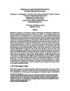
We have constructed and verified a simplified version of the ATM system described in Chapter 5. Our system, as in Chapter 5, consists of two ATM machines and one server, and contains only the operations involved in money withdrawal. But here we abstract away - as non-interesting - the operations involved in card inserting and code checking. We also left only one aspectual scenario - taking the operation fee after successful withdrawal operations. Here we also assume that the operation fee is to be taken only from some of the accounts (as it is in real life). As we are going to model-check the system, there are some abstractions to be done. We assume that there are only two bank accounts, and each of them has an initial amount of M AXBAL dollars, where M AXBAL is a constant which we chose, when constructing the example, to initialize to 3. We also assume that each transition that takes money from any account takes exactly the sum of 1 dollar. And as we said that the operation fee (denoted of ) should be taken from some of the accounts only, we decide that account no. 1 only is to pay the fee. The pseudo-code of the system is shown in Figure 6.1. (The CNV input file constructed for Stage1 of verification of the ATM system appears in Appendix A.) The aspects are woven into the system, and the result of the weaving is not only in the addition of the aspectual operations of 1 and of 2, but also in the introduction of two new variables, swl1 and swm1 (the swl1 associates with “successful withdrawal by ATM1 from account 1”, and the swm1 - with “successful withdrawal by ATM2 from account 1”). The purpose of these two variables is to adapt the enabledness of the operations of the original system to the situation of system with aspects. For example, if a user started the money-withdrawal operation at ATM1, by performing 30


Initially: wml=wmm=0, accl=accm=0, swl1=swm1=0, bal1=bal2=3 ATM 1: loop forever do ATM 2: loop forever do l1: (start withdrawal for acc.1) m1: (start withdrawal for acc.1) [l=1 /\ accl=0] [m=1 /\ accm=0] l2: (start withdrawal for acc.2) m2: (start withdrawal for acc.2) [l=1 /\ accl=0] [m=1 /\ accm=0] l3: (return card,etc.) m3: (return card,etc.) [l=2 /\ wml=0 /\ swl1=0] [m=2 /\ wmm=0 /\ swm1=0] Server: loop forever do s1: [wml=1 /\ accl=1 /\ swl1=0 /\ bal1>0] s2: [wml=1 /\ accl=2 /\ bal2>0] s3: [wmm=1 /\ accm=1 /\ swm1=0 /\ bal1>0] s4: [wmm=1 /\ accm=2 /\ bal2>0] s5: [wml=1 /\ accl=1 /\ swl1=0 /\ bal1 [c=1 /\ blen>0] m2: (await) c2: (consume a value) [m=2/\(y1=0 \/ s!=2) /\ [c=2] blen [m=3] m4: [m=4]

Advisor: loop forever do obsaspl: (count insertions for Producer 1) [obsl=1] obsaspm: (count insertions for Producer 2) [obsm=1]

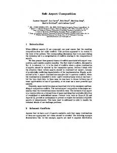
Figure 6.2: Buffer system pseudo code - first try

The pseudo-code of the first variant of the system (with aspects) is as shown in Figure 6.2. The aspects are woven into the system. The advice of the aspect counting the insertions of Producer1 is obsaspl, and obsaspm is the advice for Producer2. In our system we abstracted out the values of the counters, so the operations obsaspl and obsaspm only update their corresponding flags, obsl and obsm, to show that the aspectual advice has been performed. As in the ATM system example (Section 6.1), the flags obsl and obsm are used as an abstraction for calling the aspect advice. Those variables also, again like in Section 6.1, make the pointcuts explicit.

33


We tried to verify this system, and found out that not every pointcut is indeed followed by the corresponding aspect, because there are some inserts after which the corresponding advice is not called (i.e., the counter is not updated), which is, of course, a totally wrong behavior. As a result, there will be non-fulfilled predictions left in the history queue in some computations. The counterexample was found when checking the CorrectPredictions property, in a way similar to that of Section 6.1. It was found out that the enabledness of l1 and m1 operations was wrong: The new variables, obsl and obsm, were not used to change the enabledness of the operations of the original system. Thus it could continue with its operations and never choose the advice transition, even though it became enabled. Initially: head=blen=y1=y2=0, s=1, obsl=0, obsm=0 Producer 1: loop forever do l1: (produce a value) [l=1/\obsl=0] < y1:=1; s:=1; l:=2> l2: (await) [l=2/\(y2=0 \/ s!=1) /\ blen l3: (store the produced value) [l=3] l4: [l=4]

Producer 2: loop forever do Consumer: loop forever do m1: (produce a value) c1: (wait for a value) [m=1/\obsm=0] [c=1 /\ blen>0] < y2:=1; s:=2; m:=2> m2: (await) c2: (consume a value) [m=2/\(y1=0 \/ s!=2) /\ [c=2] blen [m=3] m4: [m=4]

Advisor: loop forever do obsaspl: (count insertions for Producer 1) [obsl=1] obsaspm: (count insertions for Producer 2) [obsm=1]

Figure 6.3: Buffer system pseudo code - corrected version

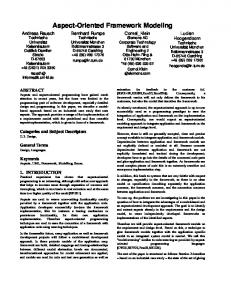
After finding the mistake, we have corrected our system, as shown in Figure 6.3. In our correction, all the following operations of that process are suspended till after the advice finishes to run. This is obtained by appropriate usage of obsl and obsm for updating the enabledness of l1 and m1. Our correction was adding the conditions on the values of the flags to the enabledness of l1 and m1. Both stages of the verification 34


of the corrected system succeeded, which shows, according to Theorem 3, that the system described in Figure 6.3 indeed conforms to its specification.

6.2.2

Detecting Risk of Overflow

Let us suppose the system described in Section 6.2.1 was constructed and ran, and it was discovered that the Producer 1 is more productive than Producer 2. Then we would like to see whether its productiveness doesn’t fill up the buffer so that there is a risk of an overflow. Thus we add the following aspect to the original Buffer system: The pointcut of the aspect is the last operation of value insertion performed by Producer 1. The advice now has two operations - the first one is updating the counter of values inserted by Producer 1, and the second one checks whether the buffer became full after the insertion (and thus detects the risk of overflow). Initially: head=blen=y1=y2=0, s=1, obsl=0, rcl=0 Producer 1: loop forever do l1: (produce a value) [l=1/\obsl=0] < y1:=1; s:=1; l:=2> l2: (await) [l=2/\(y2=0 \/ s!=1) /\ blen l3: (store the produced value) [l=3] l4: [l=4]

Producer 2: loop forever do Consumer: loop forever do m1: (produce a value) c1: (wait for a value) [m=1] [c=1 /\ blen>0] < y2:=1; s:=2; m:=2> m2: (await) c2: (consume a value) [m=2/\(y1=0 \/ s!=2) /\ [c=2] blen [m=3] m4: [m=4]

Advisor: loop forever do obsaspl: (count insertions for Producer 1) [obsl=1 /\ rcl=0] lrisk: (check the risk of overflow) [rcl=1]

Figure 6.4: Buffer system with longer advice - pseudo code

The pseudo-code of the resulting system is as shown in Figure 6.4. The difference between this system and the one shown in Figure 6.3 is only in the fact that there 35


is one aspect advice instead of two, and it has two operations and not one. The changes that the weaver made to the original system appear only in Producer1, as the advice is applied only to Producer1, and those changes are the same as were made in Figure 6.3. Both stages of the verification for the system in Figure 6.4 succeeded. Thus, according to Theorem 3, we conclude that this system indeed conforms to its specification.

36


Chapter 7 Implementation Details 7.1 7.1.1

Extended CNV Tool Implementation Using the Extended CNV

The input to the Extended CNV tool is the description of the original woven system as a transition system, together with its independence relation, the list of the non-aspectual scenarios, and the description of the aspectual scenarios and their pointcuts. The independence relation is described by a logical expression, that states the condition for two operations to be independent at a state. The scenarios - both aspectual and non-aspectual - are described as sequences of operations. This is natural enough. The only problem arises with the description of the pointcuts. In the ideal situation, for each non-aspectual scenario its pointcut would be given by a sequence of operations and an LTL past formula, as in Definition 5, and our system would automatically recognize the pointcuts thus described. Meanwhile we do not run any automatic preprocessing on the system to recognize the pointcuts, and mark the pointcuts manually. After the augmented system is constructed we manually modify the body of some function defined in our augmented system. This function takes a state and an operation as parameters and tells whether or not the result of applying the given operation on the given state it is a join-point, and of which aspect. The only description of the pointer we require from the user in the input is the name of its last operation (we need it for our internal usage - preparing the list of variants of non-aspectual scenarios containing end-of-pointcut operaions, or truncated by strictly-interrupting aspects).

37


As described in Chapter 4, we perform the verification in two stages, the input to those stages is constructed from the input described above (let us call it the original input): • In the first stage our goal is to show that the aspects are applied properly, without trying to arrange the non-aspectual scenarios operations. Thus the input to this stage is almost the same as the original input, the only difference is in the list of non-aspectual scenarios. The list is modified to contain each non-aspectual operation as a scenario on its own. • In the second stage we ignore the aspectual operations assuming them to be performed atomically at the pointcuts, and arrange the non-aspectual scenarios. Here the input is the original woven system, with the original nonaspectual scenarios list and independence relation. The aspects are also fully described, but they are marked as aspect shadows and not real aspects, to let the CNV know how to treat them. When the above input files are constructed, the Extended CNV is run on them. It creates the corresponding input files for the SMV model-checker, which are then model-checked. If the model-checking of both files succeeds, the original system conforms to its specification. All the source files of the Extended CNV, together with implementation of examples from Chapter 6 and usage instructions, appear on the web page [1]. The full CNV input file for the ATM example is also listed in Appendix A, along with explanations on the form of the input. In particular, the aspect scenarios are described using the syntax “ @ASPECT xxx PTCEND yyy [STRICT] ”, where “xxx” represents the advice operations sequence, and instead of “yyy” the list of possible end-ofpointcut operations should appear. The last part, “[STRICT]”, is optional, and indicates the fact that the described aspect is strictly interrupting. For example, the aspect taking the operation fee from account no.1 is described as “ @ASPECT of1 PTCEND s1 ”, meaning that the aspectual scenario consists of one operation - of1, and the last operation of its pointcut is s1. The user also provides the non-aspectual scenarios list, the definitions of the history state variables, and, of course, the description of transitions and state variables of the original system, together with its independence relation - in the same way it was done in the non-extended CNV system. The non-aspectual scenarios are to be recognized by the chopper of the augmented system, thus they are listed in the part defining the chopper, and each scenario op1 , . . . , opn is described by “ @CHOP op1 , . . . , opn ”. The definitions of the state variables are of 38


the form “ @STATE := ”, and the history state variables are of the form “ @HISTORY_STATE [ := ] ”, for example “ @STATE wml boolean := 0 ”, “@HISTORY_STATE accl 0”. Notice that not all the state variables are history state variables - for optimization purposes, the variables not relevant to determining independence are omitted from the history state. See Appendix A for more details.

7.1.2

Extended CNV Structure

The CNV tool as described in [5] is extended by the ability to treat aspect-containing systems. Thus there are the following differences between the augmented systems created by the previous and the extended versions of the CNV: • Different swap operations The enabledness of the swap operations is now altered according to the description in Section 4.3 in order to treat the endof-pointcut operations correctly. • Advisor module At the first stage of verification, the need of predicting the appearance of the advice after the pointcut arises. A new module, the advisor, is added to the augmented system for that purpose. Its job is to detect that a new end-of-pointcut operation has just entered the history, and to insert the appropriate prediction of the advice after it. This module is stateless, like all the other modules added to the original system, except for the history, so this addition does not influence the complexity. • Automatic extraction of advice At the second stage of the verification, we need to ignore the aspect advice in the computations. This is done by changing the effect of the end-of-pointcut operations to be the combined effect of the pointcut and its corresponding advice performed atomically together. This change of effect is performed automatically on-the-fly. The transition module, that is responsible for updating the state of the original system and of the history when any operation of the original system is performed, is altered for that purpose to treat the end-of-poincut operations in a different way. When the end-of-pointcut operation occurs in the original system, the next state of the system is advanced to the one reached by applying the advice as a whole together with the end-of-pointcut operation. • Chopping interrupted scenarios The Chopper module is modified to recognize the prefixes of scenarios cut by strictly-interrupting advice.

39


7.2

Complexity

In Chapter 4 we have described our tool and the verification process performed to check the conformance of the given system to its specification, but we have not discussed the time and memory consumption of this verification process. In our case, the verification is done by model-checking, so the size of the model of the augmented system is most important, and this size depends on the number of the variables in the augmented system state. Let M be the system given, V - the set of variables of M , and T - the set of its transitions. Let M1 ′ and M2 ′ be the augmented systems built from M as defined in Section 4.3 and Section 4.4. Then the number of variables in the augmented systems exceeds the number of variables in M by L1 ∗ (|V | + log|T |) and L2 ∗ (|V | + log|T |) respectively, where Li is the length of the history in Mi ′, as it was for the augmented system built in [5]. The reason for it is that all the modules we added to M , except for the history module, were stateless, so they didn’t add new variables to the state of the augmented system. Now it is evident that we should strive to reduce the length of the history. Let us see by what means it can be done. L1 and L2 depend on the length of the treated scenarios, and on their possible interleavings. For example, it is better not to have a scenario of length 6 but rather to have 3 scenarios of length 2 instead, in case those three scenarios can not interfere, because then we will have to reserve only 2 places in the history for those scenarios, instead of 6. In fact, if those scenarios do interfere, the worst case will be that we will have to reserve the same 6 places for them, so splitting the scenarios, if possible, can not be worse than not splitting. In our case, the argument above shows that it is better indeed to divide our verification to two stages. Indeed, let A be an aspect with advice σa = a1 , . . . , ak , and let its potential pointcut, t, appear in some scenario σ of length n. Then the number of places to be reserved in the history for σ becomes n + k instead of n, because σa will be predicted as a whole whenever t is a real pointcut of A, and thus σ and the prediction of σa will appear in the history at the same time. The table in Figure 7.1 shows that splitting the verification into two stages was worth doing. The columns of the table are as follows: The first is the verified system (described by the number of the figure in which its pseudo-code is given). The second is the number of aspectual scenarios in the system, and the third - the maximal length of the aspectual scenarios. The next two columns show the time needed to run the two stages of the verification, written in format “min:sec”, and the last column shows the time needed for verification which is not split in two stages (i.e., trying to arrange both the aspectual and the non-aspectual scenarios at the same time). The fact is that the cases where we ran the non-split verification

40


never gave any result, and always ended with a crash of the model-checker because the memory was filled up. (Notice that only the variants of the Buffer system from Section 6.2 were compared. The second stage is the same for all because the non-aspectual part of the system was the same in all the cases). System Fig 6.2 Fig 6.3 Fig 6.4

Asp. no. 2 2 1

max(|adv|) 1 1 2

Stage1 run 45:19 43:49 19:22

Stage2 run 56:53 56:53 56:53

Mixed run time ∞(memory filled up) ∞(memory filled up) ∞(memory filled up)

Figure 7.1: Time consumption of the verification, when run on 4GB Linux machine (P4 with 3.2.MHz cpu)

Along with the new optimization introduced for the case of systems with aspects, there exists another optimization useful for both aspectual and non-aspectual scenarios. It was used in the original CNV tool also. As we mentioned above, it is preferable to have many short scenarios rather than a single long one. Thus if we have a long (aspectual or non-aspectual) scenario in our specification, we can split it into short parts, the concatenation of which will give the whole scenario, and split the verification to several stages. For example, let there be a scenario σ = t1 , . . . , t6 . We will split it to three sub-scenarios, σ1 = t1 , t2 , σ2 = t3 , t4 and σ3 = t1 , t2 . Instead of verifying at one stage that the long scenario σ can be brought to appear as a block, we will do the following steps: • Show that the first part, σ1 , can be arranged as needed. • Build a new system, in which the arranged part of the scenario will be replaced by one atomic operation, op1 . • For the new built system, repeat the above steps to show that all the parts of the original scenario can also be arranged (in our case the sub-scenarios σ2 and σ3 will be arranged and replaced by atomic operations op2 and op3 respectively). • Show (maybe also by dividing the verification to several steps) that the scenario consisting of the new atomic operations (hop1 , op2 , op3 i in our example) can be brought to appear as a block. It is easily seen that the above process is indeed sound, and helps reducing the size of the history queue.

41


Chapter 8 Future Work 8.1

Full Treatment of Nested Aspects

Let A be some aspect with advice σa = a1 , . . . , an , and B - an aspect with advice σb = b1 , . . . , bn , and let us also suppose that some ai is a possible end-of-pointcut operation for B. If B is not strictly-interrupting, the verification of correct appearance of both A and B is already handled in the present version. We are left to treat the case of strictly-interrupting aspect B. In this case, there might exist a computation in which only part of the advice of A, a1 , . . . , ai , appears after the pointcut of A, as A is to be interrupted and cut by B. Thus whenever a pointcut of A occurs in some computation of the original system, we would like to predict only the relevant part of the advice σa . When verifying the conformance of M to its specification, we check reducibility of every computation of M . In each computation g′ of the currently verified augmented system, we should perform the following: Let g be the computation of M followed by g′, and let the pointcut of A occur at some state s of g. We need to examine all the states to which we can get from s by applying prefixes of σa : s1 = a1 (s), s2 = a2 (a1 (s)),. . ., sn = an (. . . (a2 (a1 (s))) . . .). We need to find the smallest j such that sj is a pointcut of some strictly-interrupting aspect. If such a j exists, we should, when arriving at s in g′, predict only a1 , . . . , aj , and if such a j doesn’t exist, the whole σa should be predicted. As we see, the treatment of this case is possible, and, moreover, it doesn’t increase the size of the constructed model.

42


8.2

Treatment of “Before” Advice

In the implemented tool at this time we treat only “After” advice, i. e., advice that follows its pointcut. But we would like to be able to show the correctness of applying “Before” advice as well. For that purpose we propose one possible solution: Let A be a “Before” aspect, with advice σa = a1 , . . . , an . • When the last operation of the pointcut of A is to be inserted to the history, the prediction of σa is inserted to the history first, in the reverse order, as follows: an , . . . , a1 . Those predictions will be fulfilled only if the advice of A indeed appears somewhere in the prefix of the history at that moment, and can be brought by legal swaps to occur immediately before the pointcut. • To optimize the re-organization process and avoid unnecessary swaps, we can define swap directions for the operations of “Before” advice and their predictions, as follows: The operations of the advice of A, once entered the history, should be swapped towards the tail of the history only, as only there they will possibly meet with their predictions. For the same reason, the predictions of those operations can only be swapped towards the head of the history. Here we saw there exists a possible solution to the problem of arranging the “Before” advice. It is rather a costly one, though, because both the advice and its predictions as a whole will appear in the history at the same time, at a moment when the pointcut is inserted. Thus the number of places in the history queue reserved for this advice would be twice as large as in case it was an “After” advice, so the size of the history significantly grows.

43


Chapter 9 Conclusions Formal methods will be useful for software development only if they both deal with specification methods actually used, and treat real languages and programming techniques. Software model checking systems such as Bandera [7] or Java Pathfinder [8] already can turn Java code into input for standard model checking. In this thesis, we show how specifications based on scenarios, like those seen in UML, can be extended to treat aspect scenarios, and how systems with aspects woven into them (e.g., the result of the AspectJ precompiler into Java bytecode) can be proven to conform with such a specification using model checking. The model produced by a software model checker applied to a woven system actually is a machine M which is the input to our system. The efficiency of the resultant model checking tasks is an obvious problem, due to the extended state of the transformed model. However, optimization techniques described in this thesis and in [5] can be used to separate this task into several smaller stages. This work thus provides another step towards the goal of integrating formal methods into practical software development.

44


Bibliography [1] http://www.cs.technion.ac.il/~ssdl/thesis/finished/2006/emilia [2] J.Araujo, J. Whittle, and D. Kim, Modeling and composing scenario-based requirements with aspects, The 12th IEEE International Requirements Engineering Conference (RE2004) (Kyoto, Japan), September 2004, pp. 58–67. [3] I. Beer, S. Ben-David, C. Eisner, and A. Landver, RuleBase: An industryoriented formal verification tool, Proceedings of the 33rd Design Automation Conference, June 1996, LNCS 1254, 1997, pp. 480483, More details at http://www.haifa.il.ibm.com/projects/verification/RB_Homepage/. [4] M. Glusman and S. Katz, A mechanized proof environment for the convenient computations proof method, Formal Methods in System Design 23 (2003), 115–142, Available at http://www.cs.technion.ac.il/Labs/ssdl/pub/conv_PVS. [5] M. Glusman and S. Katz, Model checking conformance with scenario-based specifications, Computer-Aided Verification, (CAV’03) (W.A. Hunt and F. Somenzi, eds.), LNCS, vol. 2725, Springer-Verlag, 2003, pp. 328–340, Full version and system at http://www.cs.technion.ac.il/Labs/ssdl/pub/CNV. [6] D. Harel and R. Marelly, Come, let’s play : Scenario-based programming using LSC’s and the play-engine, Springer-Verlag, 2003. [7] J. Hatcliff and M. Dwyer, Using the Bandera Tool Set to model-check properties of concurrent Java software, Proc. 12th Int. Conf. on Concurrency Theory, CONCUR’01 (K. G. Larsen and M. Nielsen, eds.), LNCS, vol. 2154, SpringerVerlag, 2001, pp. 39–58. [8] K. Havelund and T. Pressburger, Model checking Java programs using Java PathFinder, International Journal on Software Tools for Technology Transfer (STTT) 2 (2000), no. 4.

45


[9] E. Katz and S. Katz, Verifying scenairio-based aspect specifications, Formal Methods (FM’05) (J.S. Fitzgerald, I.J. Hayes and A. Tarlecki, eds.), LNCS, vol. 3582, Springer-Verlag, 2005, pp. 432–447. [10] S. Katz, Aspect categories and classes of temporal properties, Transactions on Aspect Oriented Software Development 1, LNCS 3880, 2006, pp. 106–134. [11] G. Kiczales, E. Hilsdale, J. Hugunin, M. Kersten, J. Palm, and W. G. Griswold, An overview of AspectJ, Proceedings ECOOP 2001, LNCS 2072, Jun 2001, http://aspectj.org, pp. 327–353. [12] S. Krishnamurthi, K. Fisler, and M. Greenberg, Verifying aspect advice modularly, SIGSOFT FSE, 2004, pp. 137–146. [13] Z. Manna and A. Pnueli, The temporal logic of reactive and concurrent systems - safety, Springer-Verlag, 1995. [14] K. L. McMillan, Getting started with SMV, Cadence Labs, March 1999. [15] S. Owre, N. Shankar, J.M. Rushby, and D.W.J. Stringer-Calvert, PVS Language Reference, Computer Science Lab, SRI International, Menlo Park, CA, 1998. [16] D. Peled, Software reliability methods, Springer-Verlag, 2001. [17] G. L. Peterson. Myths about the mutual exclusion problem. Information Processing Letters, 12(3):115–116, 1981. [18] J. Rumbaugh, I. Jacobson, and G. Booch, The Unified Modeling Language reference manual, second edition, Addison-Wesley, 2004. [19] D. Sereni and O. de Moor, Static analysis of aspects., AOSD, 2003, pp. 30–39. [20] M. Sihman and S. Katz, Superimposition and aspect-oriented programming, BCS Computer Journal 46 (2003), no. 5, 529–541, Available at http://www.cs.technion.ac.il/~katz/cj.ps [21] J. Whittle and J.Araujo, Scenario modeling with aspects, ISS Proceedings– Software, vol. 151, no. 4, 2004, pp. 157-172.

46


Appendix A CNV Input File for ATM Example This is the input to the first stage of the verification - arranging the aspects: (For the second stage, this file will be changed in the following way: the aspects will be declared using the key-word ASPECT_SHADOW instead of ASPECT, and the CHOP part will contain the original non-aspectual scenarios list, and not just the list of non-aspectual operations) ##-------------------------------------------------------------## System description: Two ATM machines and a server. ## Specification : money withdrawal scenario - non-aspectual; ## taking operation fee scenario - aspectual, executed after ## successful withdrawal operation ## The unsuccessfull withdrawal operations are also defined here. ## ## Only part of bank accounts is obliged to pay operation fee ## our abstraction : account no.1 only has to pay ## ## Initially: wml=wmm=0, accl=accm=0, swl1=swm1=0, bal1=bal2=3 ## ATM 1: loop forever do ## [LAZY] l1: //start withdrawal for acc. 1 ## [l=1 /\ accl=0] ## [LAZY] l2: //start withdrawal for acc. 2 ## [l=1 /\ accl=0] ## l3: //return card,etc. ## [l=2 /\ wml=0 /\ swl1=0] ## ATM 2: loop forever do ## [LAZY] m1: //start withdrawal for acc. 1 ## [m=1 /\ accm=0] ## [LAZY] m2: //start withdrawal for acc. 2 ## [m=1 /\ accm=0] ## m3: //return card,etc. 47


## [m=2 /\ wmm=0 /\ swm1=0] ## Server: loop forever do ## s1: [wml=1 /\ accl=1 /\ swl1=0 /\ bal1>0] ## ## s2: [wml=1 /\ accl=2 /\ bal2>0] ## ## s3: [wmm=1 /\ accm=1 /\ swm1=0 /\ bal1>0] ## ## s4: [wmm=1 /\ accm=2 /\ bal2>0] ## ## s5: [wml=1 /\ accl=1 /\ swl1=0 /\ bal10 @ASSIGN wml := 0 @ASSIGN bal2 := bal2-1 @END @TRANS s3 @ENABLE wmm=1 & @ASSIGN swm1 := @ASSIGN wmm := @ASSIGN bal1 := @END

accm=1 & swm1=0 & bal1>0 1 0 bal1-1

@TRANS s4 @ENABLE wmm=1 & accm=2 & bal2>0 @ASSIGN wmm := 0 @ASSIGN bal2 := bal2-1 50


@END @TRANS s5 @ENABLE wml=1 & @ASSIGN swl1 := @ASSIGN wml := @ASSIGN accl := @END

accl=1 & swl1=0 & ~(bal1>0) 0 0 0

@TRANS s6 @ENABLE wml=1 & accl=2 & ~(bal2>0) @ASSIGN wml := 0 @ASSIGN accl := 0 @END @TRANS s7 @ENABLE wmm=1 & @ASSIGN swm1 := @ASSIGN wmm := @ASSIGN accm := @END

accm=1 & swm1=0 & ~(bal1>0) 0 0 0

@TRANS s8 @ENABLE wmm=1 & accm=2 & ~(bal2>0) @ASSIGN wmm := 0 @ASSIGN accm := 0 @END @TRANS of1 @ENABLE swl1=1 & bal1>0 @ASSIGN swl1 := 0 @ASSIGN bal1 := bal1-1 @END @TRANS of3 @ENABLE swm1=1 & bal1>0 @ASSIGN swm1 := 0 @ASSIGN bal1 := bal1-1 @END ###-------------------------------------------------------------51


### Definition of the state info that must be kept in the history. ### This info must be enough to: ### - Support the definition of the conditional independence ### (see below). ### - Allow updating this info with the effect of executing any ### transition. ### It is OK to use fields from the system state. ### For new fields, the type must be given. ### ### NOTE: When doing swaps of predictions in the history, the ### history state info must be updated. For the state fields that ### are also in the history, the update is done according to the ### transitions’ @ASSIGN statements. Likewise, the assignment ### to be done to any other history state fields must be also ### defined in the @ASSIGN part of every transition’s definition. ### ### Format: (may use any number of times) ### NOTE: MUST NOT CONTAIN SPACES! ### Use a #define to create a name for a complex expression, ### if needed. ### @HISTORY_STATE [ := ] @HISTORY_STATE accl 0 @HISTORY_STATE accm 0 @HISTORY_STATE bal1 3 ###-------------------------------------------------------------### Independence information: ### Format: (Use exactly once) ### @INDEP ### predicate ### @END ### This predicate must characterize when transitions "tr1" and ### "tr2" are independent, possibly based on the history state ### fields recorded in the history (it must not consider ### anti-transitions). It may consider every pair of transitions ### only once, i.e., in one direction. ### The complete symmetrical independence predicate is basically: ### tr1~=tr2 & (INDEP(tr1,tr2,st) | INDEP(tr2,tr1,st)) @INDEP ( ( proc(tr1)=atm1 & (proc(tr2)=atm2 | 52


) (

) (

tr2 in {s3,s4,s7,s8} | (accl~=1 & (tr2 in {of1,of3})) ) | proc(tr1)=atm2 & (proc(tr2)=atm1 | tr2 in {s1,s2,s5,s6} | (accm~=1 & (tr2 in {of1,of3})) ) | (tr1 = of1 & (tr2 in {s4,s8} | (tr2 in {s3,of3} & bal1>1))) | (tr1 = of3 & (tr2 in {s2,s6} | (tr2 in {s1,of1} & bal1>1))) | (tr1 = s1 & (tr2=of3 & bal1>1)) | (tr1 = s2 & tr2=of3) | (tr1 = s3 & (tr2=of1 & bal1>1)) | (tr1 = s4 & tr2=of1) | (tr1 = s6 & tr2=of3) | (tr1 = s8 & tr2=of1)

) ) @END ###-------------------------------------------------------------### To use a stateless "convenient prefix" recognizer: ### Specify sequences of transitions that, if found as a prefix of ### the history, can be chopped from it. ### Format: (Use repeatedly, from highest to lowest precedence) ### @CHOP tr1 tr2 tr3 ... @CHOP l1 @CHOP l2 @CHOP l3 @CHOP m1 @CHOP m2 @CHOP m3 @CHOP s1 @CHOP s2 @CHOP s3 @CHOP s4 @CHOP s5 @CHOP s6 @CHOP s7 53


@CHOP s8 ###-------------------------------------------------------------### To define an aspectual scenario, specify its advice as a ### sequence of operations, and list all ### the possile end-of-pointcut operations. ### Format: (UseRepeatedly) ### @ASPECT xxxxx PTCEND yyyyy [STRICT] ### the advice sceanrio is to be inserted in place of "xxxxxx", ### the word PTCEND is followed the list of possible last operations ### of the pointcut ### (space is the separator) ### [STRICT] - optional flag. When appears, it means that the aspect ### is strictly interrupting. @ASPECT of1 PTCEND s1 @ASPECT of3 PTCEND s3 ###-------------------------------------------------------------### This creates a predictor. ### Format: (Use repeatedly, from highest to lowest precedence) ### @PREDICT tr4 tr5 ... AFTER tr1 tr2 ... tr3 ### This will insert "tr4 antitr4" after the prefix "tr1 tr2 tr3", ### then "tr5 antitr5" after the prefix "tr1 tr2 tr3 tr4" ### (before antitr4), etc. ### or ### @PRED tr4 ... tr5 tr6 AFTER tr1 tr2 ... tr3 ### This will insert "tr4 antitr4" after the prefix "tr1 tr2 tr3", ### "tr5 antitr5" after "tr1 tr2 tr3 tr4" and before "antitr4",... ### and finally replace the prefix "tr1 tr2 tr3 ... tr5" with ### antitr6, i.e., the prefix "tr1 tr2 tr3 ... tr5 tr6" is ### chopped immediately. ###-------------------------------------------------------------### Define the number reserved history cells, needed to accomodate ### non-chopping predictions that may need to be done even when the ### history is full. ### Format: (use at most once. Default: 0) ### @RESERVED n @RESERVED 0

54


###---###---###---###---###---###---###---###---###---###---###-### WARNING: ALL the @GENERATE* commands MUST come after all the ### other @ commands. ###-------------------------------------------------------------###-------------------------------------------------------------### Add here example-specific defines #define MAXBAL 3 #define proc(tr) case {tr in {l1,l2,l3} : atm1; \ tr in {m1,m2,m3} : atm2; \ tr in {s1,s2,s3,s4,s5,s6,s7,s8} tr in {of1,of3} : advisor; default : none; }

: server;\ \

## ## Uncomment this #define if you want to do only model emptiness ## check. Alternatively, run smv with the command-line argument ## "-DCHECK_EMPTINESS" ## #define CHECK_EMPTINESS ## Uncomment this #define to check only the user-defined ## independence. Alternatively, use "smv -DCHECK_INDEP ..." ## #define CHECK_INDEP @GENERATE_DEFINES ###-------------------------------------------------------------### Add here example-specific typedefs typedef b_index 0..MAXBUFLEN-1; typedef values boolean; typedef mpc 1..2; typedef acc 0..2; typedef procs {atm1,atm2,server,advisor,none}; @GENERATE_TYPEDEFS ###-------------------------------------------------------------### Add here example-specific modules

55


###-------------------------------------------------------------### This generates the transitions’ modules and includes other ### modules from "common_modules.smv" @GENERATE_MODULES ### This generates the beginning of module main @GENERATE_MODULE_MAIN ### You may add here your own stuff for the main module ###-----------------------------------------------### Checking the reduction for a single computation: ### To check if (and how) a single computation (that can be ### defined by an LTL formula) can be reduced to a convenient one, ### uncomment the following assertion. ### (and complete the description of the single computation). ### If this assertion holds, there is NO reduction. Otherwise, ### the counterexample shows a reduction in detail. ### ### check_interesting_comp: assert ### ( WriteHereYourLTLdescriptionOfTheComputation ) -> F error; ### ### Hints: ### 1- The macro "system_running" describes the states in which a ### transition of the system is being taken. ### 2- To describe that after transition tr1, tr2 will occur, ### you can uncomment and use this macro: ### #define seq(tr1,tr2) \ ### (inst.tr1.running->X(~system_running U inst.tr2.running)) ### ###-----------------------------------------------### This defines the reduction specification (red_conv) and closes ### the module main @GENERATE_SPECIFICATION

56


‫אימות של מפרטי אספקטים‬ ‫המבוססים על תרחישים‬

‫אמיליה כץ‬

‫חיבור על מחקר‬

‫לשם מילוי חלקי של הדרישות לקבלת התואר‬ ‫מגיסטר למדעים במדעי המחשב‬

‫אמיליה כץ‬

‫הוגש לסנט הטכניון – מכון טכנולוגי לישראל‬ ‫פברואר ‪2006‬‬ ‫חיפה‬ ‫שבט תשס"ו‬

‫‪Technion - Computer Science Department - M.Sc. Thesis MSC-2006-08 - 2006‬‬

‫אימות של מפרטי אספקטים המבוססים על תרחישים‬

‫ברצוני להודות מקרב לב למנחה שלי‪ ,‬פרופ"ח שמואל כ"ץ‪ ,‬על הנחייתו ותמיכתו‬ ‫לאורך כל הדרך‪.‬‬


‫המחקר נעשה בהנחיית פרופ"ח שמואל כ"ץ בפקולטה למדעי המחשב‪.‬‬ ‫אני מודה ל ‪ AOSD-EUROPE Network of Excellence‬על התמיכה הכספית‬ ‫הנדיבה בהשתלמותי‪.‬‬

‫‬

‫‬

‫‬

‫‬

‫‬

‫‬ ‫ ‬

‫‬

‫‬

‫‬

‫‬

‫‬

‫‪ 1.1‬פרטים מבוססי תרחישים‪2...............................................................................‬‬ ‫‪ 1.2‬אספקטים ותרחישים‪2.....................................................................................‬‬ ‫ ‬ ‫‬

‫ ‬

‫‬

‫‬

‫‬

‫‬

‫ ‬

‫‬

‫ ‬

‫‬

‫ ‬

‫‬

‫‪ 2.1‬הגדרה ואימות מערכות עם אספקטים‪6..............................................................‬‬ ‫‪ 2.1.1‬הגדרת אספקטים על‪-‬ידי תרחישים‪6......................................................‬‬ ‫‪ 2.1.2‬אימות מודולרי‪6.................................................................................‬‬ ‫‪ 2.2‬אימות מערכות ללא אספקטים‪7.......................................................................‬‬ ‫‪ 2.2.1‬הוכחת משפטים )‪7.................................................(Theorem Proving‬‬ ‫‪ 2.2.2‬בדיקת מודלים )‪8.....................................................(Model Checking‬‬ ‫‬

‫‬

‫‬

‫‬

‫‬

‫‬

‫‬

‫‬

‫‬

‫‬

‫‪CNV‬‬ ‫‬

‫‬

‫ ‬

‫‬

‫‬

‫‬

‫‬

‫‬

‫‪4.1‬‬ ‫‪4.2‬‬ ‫‪4.3‬‬ ‫‪4.4‬‬ ‫‪4.5‬‬

‫‬

‫‬

‫‬

‫‬

‫‬

‫‬

‫ ‬

‫‬

‫‬

‫‬

‫‬

‫‬

‫‬

‫‬

‫ ‬

‫הגדרת הבעיה‪12...........................................................................................‬‬ ‫זיהוי ה – ‪ : pointcuts‬ארבע אפשרויות‪14............................................................‬‬ ‫הבטחת הופעת האספקטים‪15..........................................................................‬‬ ‫סידור התרחישים הלא‪-‬אספקטיים‪18.................................................................‬‬ ‫הוכחת נאותות‪20...........................................................................................‬‬

‫‬

‫‬

‫‬

‫‬

‫‬

‫‬

‫‬

‫‬

‫‬

‫‬

‫‬

‫‬ ‫‬

‫‬

‫‬

‫‬

‫‬

‫‬

‫‬

‫‬

‫ ‬

‫‬

‫‬

‫‬

‫‬

‫ ‬

‫‬

‫‬

‫‬

‫‬

‫‬

‫‬

‫‬

‫ ‬

‫‪ 6.1‬דוגמת מערכת הכספומטים‪30..........................................................................‬‬ ‫‪ 6.2‬דוגמת מערכת ה – ‪32.................................................................................. Buffer‬‬ ‫‪ 6.2.1‬בדיקת ביצועי היצרנים‪33......................................................................‬‬ ‫‪ 6.2.2‬גילוי הסיכון לגלישה‪35.........................................................................‬‬ ‫‬ ‫‬

‫‬

‫‬

‫‪7.1‬‬

‫‬

‫‬

‫‬

‫‬

‫‬

‫‬

‫‬ ‫‬

‫מימוש כלי ה – ‪ CNV‬המורחב‪37.....................................................................‬‬ ‫‪ 7.1.1‬שימוש ב – ‪ CNV‬המורחב‪37..............................................................‬‬


‫תוכן העניינים‬


39................................................................‫ המורחב‬CNV – ‫ מבנה ה‬7.1.2 40...................................................................................................‫סיבוכיות‬

7.2

42....................................................................‫טיפול מלא באספקטים מקוננים‬

8.1

43......................................................................."Before" Advice – ‫טיפול ב‬

8.2

4

CNV


‫‪6.1‬‬ ‫‪6.2‬‬ ‫‪6.3‬‬ ‫‪6.4‬‬ ‫‪7.1‬‬

‫פסאודו‪-‬קוד של מערכת הכספומטים‪30...................................................................‬‬ ‫פסאודו‪-‬קוד של מערכת ה – ‪ : Buffer‬נסיון ראשון‪32................................................‬‬ ‫פסאודו‪-‬קוד של מערכת ה – ‪ : Buffer‬גרסא מתוקנת‪33............................................‬‬ ‫פסאודו‪-‬קוד של מערכת ה – ‪ Buffer‬עם ‪ advice‬ארוך יותר‪34.....................................‬‬ ‫צריכת הזמן של האימות על מחשב ‪ P4) 4GB ,Linux‬עם ‪38..................(3.2 MHz cpu‬‬


‫רשימת טבלאות וציורים‬


$

%

!

$

"

#

!

UML

(

&

'

Live Sequence Charts (LSCs)

)

$

! /

$

.

& !

'

*

+

,

-

*

,

0

0

0

2

*

3

0

1

(

4

3

5

6

7

$

"

"

!

AspectJ

advice

pointcut

advice

(

(join-points)

security

0

1

(

(weave)

$

1

0

1

1

8

!

monitoring

0

0

(

i

(


(

(

0

(

1

s

(

s

"

!

$

"

!

$

8

!

s

1

(spectative aspects)

0

$

communication failure

1

(invasive aspects)

(regulative)

(

(

0

(

'

(

&

woven in

0

weaver

1

ii


' &

augmented system

(

&

'

0

(

0

(

'

&

strict interruption

1

&

(

'

weak interruption

1

(

&

'

$

(

! /

CNV

model-checking

1

(

0

(

model-checking

(

1

(

strictly interrupting aspect

&

(

)

(

(

pointcut

&

'

pointcut

)

after advices

#

)

)

before

1

iii

(

1

advices

1


"

8

(

(

&

(

0

'

(

0

0

(

pointcut

)

pointcut

(

1

(

(

0

0

(

(

(

0

iv

Verifying Scenario-Based Aspect Specifications - CiteSeerX

Verifying Scenario-Based Aspect Specifications - CiteSeerX

Suggest Documents

Verifying Model Oriented Specifications through Animation

Verifying Modal Workflow Specifications using ... - Semantic Scholar

Implementing and Verifying Message Sequence Chart Specifications

Implementing and Verifying MSC Specifications ... - KOPS Konstanz

Verifying Correctness in StAC Specifications - Semantic Scholar

Verifying Controlled Components - CiteSeerX

On Verifying Consistency of XML Specifications - University of Toronto ...

Assertion with Aspect - CiteSeerX

Verifying Business Process Compatibility - CiteSeerX

Organization Aspect - CiteSeerX

Aspect Oriented Framework - CiteSeerX

Safe Aspect Composition - CiteSeerX

Aspect-oriented Requirements - CiteSeerX

Aspect Oriented Programming - CiteSeerX

Style specifications thesis - CiteSeerX

Refactoring Alloy Specifications - CiteSeerX

Analysing Inconsistent Specifications - CiteSeerX

Style specifications thesis - CiteSeerX

Style specifications thesis - CiteSeerX

Style specifications thesis - CiteSeerX

Restructuring Requirements Specifications - CiteSeerX

Experiences in Specifications - CiteSeerX

Aspect for thicj layered... - CiteSeerX

Aspect-Oriented Framework Modeling - CiteSeerX