Verifying the Solution from a Nonlinear Solver: A Case Study - CiteSeerX

Verifying the Solution from a Nonlinear Solver: A Case Study By B. D. MCCULLOUGH The probit is generally considered to be one of the easiest nonlinear maximum likelihood problems. Nonetheless, in the course of attempting to replicate G. S. Maddala’s (1992, pp. 335–38) probit example, Houston Stokes (2003) encountered great difficulty. Of the six coefficients, five coefficients/standard errors he could duplicate, but the sixth was off by more than rounding error. So he tried another package. And another. And another ... . Finally, five different packages had declared convergence to five solutions that differed only in the sixth coefficient. Estimates of the sixth coefficient ranged from 4.4 to 8.1, and estimates on its standard error ranged from 46 to 114,550. For each of the packages that produced an answer, Stokes decreased the convergence tolerance and always found that the five coefficient/standard error pairs did not change, but the sixth coefficient usually changed appreciably. Often the sixth coefficient doubled in size, and the sixth standard error always increased dramatically. Curiously, despite large changes in the sixth coefficient, the LogL (log-likelihood) did not change. What could have gone wrong? It might seem that the problem is overparameterized and that the sixth parameter is superfluous, but that

AND

H. D. VINOD*

would be too easy. In fact, the difficulty is that for the particular set of data, the maximum likelihood estimator does not exist, i.e., there is no set of parameters that maximizes the likelihood.1 Observe that nonexistence was no impediment to five solvers declaring not only that a solution existed, but that the solution had been located. For sake of completeness we note that another two packages did refuse to produce an answer because they recognized that the maximum likelihood estimator did not exist—the developers of these packages had written their programs to examine the data for possible signs of nonexistence of the solution. One of the five packages that produced a solution is similarly programmed, but it failed to detect the nonexistence of the solution. If something reputedly so simple as probit estimation can fool such an experienced econometrician as Maddala, then all economists had best be on their guard, lest they be misled by their nonlinear solvers. As Stokes’ example makes clear, from the fact that a computer software package produces a solution to an estimation problem, it does not necessarily follow that the solution is accurate, or even that a solution exists. Indeed, it has been shown elsewhere (McCullough, 1999a, b, 2000a; McCullough and Berry Wilson, 1999, 2002; Vinod, 2000a) that, even under the most propitious circumstances, a nonlinear solver can produce an inaccurate answer; and in practice, circumstances rarely are propitious. Researchers conducting nonlinear estimation typically make no effort to guard against such inaccurate answers. We surveyed the past five

* McCullough: Department of Decision Sciences and Department of Economics, Drexel University, Philadelphia, PA 19104 (e-mail: [email protected]); Vinod: Department of Economics, Fordham University, New York, NY 10458 (e-mail: [email protected]). We are most grateful to W. Greene, R. Mittelhammer, and S. Nash for illuminating discussions of the ill-conditioned Hessian problem, and to R. Boik and S. Murphy for advice on likelihood profiles. For comments and technical suggestions we thank C. Cummins of TSP International and R. Schoenberg of Aptech Systems, as well as D. Erdman, J. Gentle, W. Gould, J. G. MacKinnon, M. Nerlove, J. Racine, and P.-M. Seidel. Participants at the 2001 Yale Conference on Computing in Economics and Finance made useful suggestions, as did R. Geddes, R. Kieschnick, D. Letson, and D. Reagle. We are indebted to Professors Shachar and Nalebuff for their commitment to the AER replication policy. Finally, we thank O. Ashenfelter, B. Bernanke, J. Duvall, and B. Goffe for encouragement.

1 Specifically, the data exhibited “quasi-complete separation,” a special pattern between the values of the binary dependent variable and a dummy independent variable. See A. Albert and J. Anderson (1984) for technical details. This phenomenon should be of great import to all who run probit and logit models, but it seems to be missing from the discussion of limited dependent variables in most econometrics texts; Russell Davidson and James G. MacKinnon (2003) is an exception.

873

874

THE AMERICAN ECONOMIC REVIEW

years of this journal, examining articles that presented the results of nonlinear estimation. Not a single researcher reported any attempt to verify the solution produced by his software. This may be due to the fact that this aspect of nonlinear estimation is not something in which most economists are trained. We surveyed ten econometrics texts; while each advocated the use of computer software to produce a solution to nonlinear estimation problems, none suggested verifying the solution produced by a software package. The general position of econometrics texts and researchers is that the “solution” produced by a nonlinear solver may be accepted uncritically.2 This position needs to be changed. Experienced users of nonlinear optimization routines will vary the default options of the nonlinear solver: decrease the tolerance, switch the convergence criterion, change algorithms and starting values, etc. Another good approach is to use more than one package to solve the same problem, as Stokes (2003) suggested. Of course, using more than one package tends to raise more questions than it answers for some procedures, especially those procedures for which it is well-known that different packages typically produce different answers to the same problem, e.g., ARMA models (Paul Newbold et al., 1994) and GARCH models (McCullough and Charles G. Renfro, 1999).3 Varying the default options and using more than one package, when successful, only locate a possible solution. Researchers need some means of verifying a possible solution. In this paper we advocate four steps that researchers can use to verify the solution produced by their software. We apply these steps to an example from the recent literature. 2 Some texts hint that solutions might not be accurate. Ron C. Mittelhammer et al. (2000) alerts the reader to serious numerical problems that can arise in nonlinear estimation (Sec. 8.13), and provides numerical examples of some pitfalls (e.g., Examples 8.2.3 and 8.13.3). Davidson and MacKinnon (1993, pp. 176 –78) explains how artificial regressions can be used to verify first-order conditions for nonlinear regression, and OPG regressions can be used for verifying first-order MLE conditions (p. 472). 3 McCullough and Renfro (1999) proposed the use of the FCP (Gabrielle Fiorentini et al., 1996) GARCH benchmark as a resolution to this problem. Software developers appear to be standardizing their GARCH procedures on this benchmark, as shown by Chris Brooks et al. (2001). Regrettably, there are far too few benchmarks.

JUNE 2003

I. Maximizing a Likelihood

We wish to dissociate ourselves from the standard textbook approach to nonlinear maximum likelihood estimation, but first, some background information is in order. The usual t-statistics and confidence intervals (Wald intervals) that are produced as output from nonlinear estimation routines are easy to compute and are routinely provided by most computer programs, which explains their popularity. As these t-statistics and Wald intervals (and also Wald confidence regions) are based on a quadratic approximation to the log-likelihood, they will be accurate only if the log-likelihood is approximately quadratic over the region of interest. When the log-likelihood is approximately quadratic, Wald intervals and likelihood intervals will be quite similar. When the log-likelihood is not approximately quadratic—which is more likely the more nonlinear is the problem—then the two intervals diverge and the Wald interval cannot be relied upon safely. George E. P. Box and Gwilym M. Jenkins (1976, p. 226) eloquently argued against the traditional textbook approach: The treatment afforded the likelihood method has, in the past, often left much to be desired, and ineptness by the practitioner has on occasion been mistaken for deficiency in the method. The treatment has often consisted of 1. differentiating the log-likelihood and setting first derivatives equal to zero to obtain the maximum likelihood (ML) estimates; 2. deriving approximate variances and covariances of these estimates from the second derivatives of the loglikelihood or from the expectation of the second derivatives. Mechanical application of the above can, of course, produce nonsensical answers. This is so, first, because of the elementary fact that setting derivatives to zero does not necessarily produce maxima, and second, because the information which the likelihood function contains is only fully expressed by the ML estimates and by the second derivatives of the loglikelihood, if the quadratic approximation is adequate over the region of interest. To

VOL. 93 NO. 3

MCCULLOUGH AND VINOD: VERIFYING THE SOLUTION

know whether this is so for a new estimation problem, a careful analytical and graphical investigation is usually required. When a class of estimation problems (such as those arising from the estimation of parameters in ARMA models) is initially being investigated, it is important to plot the likelihood function rather extensively. After the behavior of a particular class of models is well understood, and knowledge of the situation indicates that it is safe to do so, we may take certain shortcuts[.] Other than ARMA models, we are unaware of any class of models for which the accuracy of the quadratic approximation has been verified. This does not mean that all t-statistics from all nonlinear regressions are invalid; it only means that they have not been validated. Certainly such investigations would be of great import, especially if it was found that the quadratic approximation did not hold for a certain class of models. As an example of a specific case, Jurgen Doornik and Marius Ooms (2000), who plotted the likelihood function rather extensively, showed that the quadratic approximation does not hold in their ARCH, GARCH, and EGARCH analyses of a stock market index. Whether this is generally true of GARCH models is an open question. Aside from the validity of the t-tests on coefficients, obtaining valid point estimates from a nonlinear regression is more than a matter of simply letting the computer do all the work. ARMA models are not necessarily easily estimated: ARMA( p, q) with small q usually is easy, but even a linear model with AR(1) errors can have multiple extrema. Box-Cox models generally are not too much trouble, as long as the likelihood is concentrated. Doornik and Ooms (2000) suggested that GARCH models may be prone to multimodality, which would greatly complicate their estimation. A user ought not just accept the program’s output uncritically; rather, the user should interact with the software to test and probe the putative solution before accepting it. Too often, researchers simply accept at face value a software package’s declaration of “convergence” and think that the point estimate so obtained maximizes a likelihood or minimizes a sum of squares. However, as Stokes’ example showed, even with something so seemingly simple as a

875

probit model, these “convergence” messages are not to be trusted blindly. Indeed, this problem has even surfaced in the New York Times (Andrew Revkin, 2002), which reported that the link between soot in the air and deaths had been markedly overstated by researchers on a landmark air pollution study because “Instead of adjusting the program to the circumstances they were studying, they used standard default settings for some calculations.” Specifically, the researchers had used default settings for Generalized Additive Model (GAM) estimation, a nonlinear procedure, and the researchers unwittingly obtained false convergence. Science magazine reported that the researchers used the procedure for five years before they caught onto the problem (J. Kaiser, 2002). The errors led the Environmental Protection Agency to delay the scheduled implementation of new regulations. Of course, if the errors had not been discovered, the wrong regulations would have been put into effect, and nobody would ever have known the difference. We note that the title of the Science article suggested that a “software glitch” was to blame, but this is incorrect. Nothing was wrong with the software in question: the incorrect results were solely attributable to user error. A researcher should carefully examine any solution offered by a package, to ensure that a false maximum has not been reported.4 Many solvers conflate the concepts of “stopping rule” and “convergence criterion,” which can make it difficult for the user to know whether optimality conditions hold at a reported maximum. If the convergence criterion is “relative parameter convergence,” the solver can stop and report “convergence” even though the gradient is far from zero. This can also happen when the function value is used as the convergence criterion. Colin Rose and Murray Smith (2002, Sec. 12.3) examined an ARCH model where the program reports convergence based on the value of the objective function, yet a very small change in the LogL from 243.5337516 to 243.5337567 converts a nonzero gradient to a zero gradient. To make the matter even more complicated, due to the limitations of finite precision calculation, a reported zero gradient does not imply an

4

McCullough and Renfro (2000) discussed the reasons that a nonlinear solver can fail.

876


extremum, or even a saddlepoint. McCullough (2003) analyzed a “solution” for which each component of the gradient was numerically zero, but the point was subsequently shown to be not a valid solution—it was just in a very flat region of the surface. Either intentionally or unintentionally, it is fairly easy to trick a solver into falsely reporting an extremum—whether a maximum for likelihood estimation, or a minimum for leastsquares estimation. Therefore, the researcher’s job is not done when the program reports convergence—it is only beginning. Rather than simply relying on a computer-generated convergence message, we recommend the following checks for verifying a reported solution, say, ␤ˆ , to a nonlinear optimization problem: 1. Examine the gradient—is it zero? 2. Inspect the solution path (i.e., trace)— does it exhibit the expected rate of convergence? 3. Evaluate the Hessian, including an eigensystem analysis—is the Hessian negative definite? Is it well-conditioned? Philip E. Gill et al. (1981, p. 313) noted that if all these conditions hold then ␤ˆ “is likely to be a solution of the problem regardless or not of whether the algorithm terminated successfully” [emphasis in the original]. These three points only address the issue of whether a point estimate is locally valid or spurious—whether inference can be sustained also must be considered. Therefore, to the above three steps we add a fourth: 4. Profile the likelihood to assess the adequacy of the quadratic approximation. Thus, we advocate a departure from the usual textbook approach to nonlinear estimation. The reason for the fourth step is that standard practice for nonlinear estimation is to test hypotheses, especially concerning coefficients, using a Wald-type statistic (with the concomitant asymptotic normal approximation) that is based on a quadratic approximation to the likelihood function. Further, standard practice also pays little attention to whether the quadratic approximation is valid, in part because students are frequently given the impression that the Wald and likelihood approaches provide equally accurate approximations [e.g., C. R. Rao (1973,

JUNE 2003

p. 418)]. Rarely are students informed that there can be substantial differences between the two approaches, e.g., the Walter W. Hauck-Allan Donner (1997) phenomenon in the binary logit model [see also W. N. Venables and B. D. Ripley (1999, p. 225)]. For many years, this overemphasis on the Wald statistic at the expense of likelihood-based inference was justified on the basis of the extreme computational burden attached to the latter. In the present day, this burden is ever-decreasing, and the advantages of likelihood-based methods are becoming more widely recognized (William Q. Meeker and Luis A. Escobar, 1995, Sec. 3.1). Below we implement the four steps, but first a word of caution. These four steps cannot be accommodated by many software packages. Some packages will not permit the user to display the gradient at the solution, even though the optimization routine makes use of the gradient. There are packages that do not permit the user to access the trace. (Why a software developer would not permit the user to access the gradient or trace is beyond our understanding, but it is fairly common.) There are packages that do not have the ability to compute the Hessian at the solution.5 Lastly, there are packages for which profiling an objective function will be an unduly onerous programming exercise, if it can be done at all. II. Posing the SN Problem

We illustrate the four steps using a recently published paper as a case study (Roni Shachar and Barry Nalebuff, 1999; hereafter “SN”). SN presented a model of political participation incorporating the “pivotal-leader theory.” They presented a number of empirical findings, most of which do not concern us here. We focus only on results from one table in their paper, Table 9, which provided estimates of an econometric model based on their theoretical analysis. We are drawn to consider the results of Table 9 because, simply from a numerical perspective, we consider estimation of a 42 parameter highly nonlinear model to be quite challenging— 5

Some packages offer an “approximate Hessian” based on quasi-Newton estimation, and claim that it closely approximates the true Hessian when the number of iterations exceeds the number of parameters. Such claims cannot be relied upon safely. See McCullough (2003) for a counterexample and further details.

VOL. 93 NO. 3


877

TABLE 1—COEFFICIENTS Parameter

␴␧ ␤ 0d ␤ r0 ␳ ␩ S ␤Governor’s Race ␤Rain ␤Jim Crow ␤Income ␤Black ␤Moved In ␤Education External states (Hawaii, Alaska) 1988 1984 1980 1976 1972 1968 1964 1960 1956 1952 ␴d b0 Gallup poll GNP growth Incumbent VP candidate’s home state Presidential candidate’s state ADA and ACA scores Previous vote Previous (8 years) vote State legislature State economic growth South (1964) Southern Democrat South (1964) West (1976 and 1980) North Central (1972) New England (1960 and 1964)

SN Table 9

SN solution

TSP solution

0.1156 ⫺1.129 ⫺0.8581 0.5855 0.1490 0.0790 0.4517 ⫺0.0806 ⫺0.3510 0.2186 ⫺1.001 ⫺0.0329 0.3613 ⫺0.1770 0.0468 0.1207 0.0326 0.1465 0.1653 0.0172 0.3289 0.2646 0.2049 0.2679 0.0378 0.2932 0.0052 0.0209 0.0132 0.0195 0.0605 0.0004 0.0033 0.0025 0.0004 0.0063 ⫺0.1443 0.0776 ⫺0.0928 ⫺0.0713 0.0569 0.0679

0.1156101700 ⫺1.1301832000 ⫺0.8589113000 0.5866155200 0.000014910489 0.0787609210 0.0451949580 ⫺0.0794654810 ⫺0.3511115100 0.2189969300 ⫺1.0003932000 ⫺0.0329552240 0.3623056000 ⫺0.1771466800 0.0466542300 0.1206201900 0.0324726190 0.1464833000 0.1650568900 0.0172931310 0.3290525500 0.2648168800 0.2049925800 0.2681945500 0.0378479270 0.2933971200 0.0051469912 0.0209020940 0.0132008310 0.0194944560 0.0604774540 0.0003582359 0.0033246381 0.0025325467 0.00036951962 0.0063127442 ⫺0.1445717800 0.0776463400 ⫺0.0924887490 ⫺0.0712441380 0.568731200 0.0679576260

0.1567 ⫺1.337 ⫺0.8897 0.7906 0.0000105 0.0672 0.0608 ⫺0.1517 ⫺0.3521 0.2474 ⫺1.185 ⫺0.0369 0.3454 ⫺0.1829 0.1713 0.2416 0.1521 0.2667 0.2887 0.1087 0.4661 0.3475 0.3042 0.3627 0.0376 0.3406 0.0050 0.0204 0.0133 0.0178 0.0565 0.0004 0.0032 0.0025 0.0004 0.0061 ⫺0.1446 0.0757 ⫺0.0876 ⫺0.0714 0.0554 0.0631

especially when it is done with numerical derivatives.6 SN estimated the model by nonlinear maximum likelihood, using the “maxlik” routine of the software package GAUSS, with the algorithm, tolerance, convergence criterion, and 6 Generally speaking, analytic derivatives are superior to numerical derivatives. There are two ways to produce analytic derivatives for nonlinear estimation: symbolic differentiation and automatic differentiation. The latter is often preferable because it can handle much more complicated functions. See C. H. Bischof et al. (2002) for a discussion. We note Aptech Systems has been developing on an automatic differentiation system, and this capability should be added to GAUSS in the not-too-distant future.

method of derivative calculation all left at their default settings. Their data set contained 539 observations on 41 variables, spanning 50 states and 11 elections. SN presented estimates of the coefficients of this model in their Table 9 (reproduced in column 2 of our Table 1). The basis of their estimation is the following likelihood, given by their equation (13): (SN13) L共⍀兲 ⫽ ⌸ j50⫽ 1 ⌸ t11⫽ 1 f 2 共DP jt 兩DV jt , x jt , ␨ jt , N jt , Electoral Votesjt ; ⍀兲䡠 f 1 共DV jt 兩 ␨ jt , ⍀兲

878


where, from their equation (11): (SN11) f 1 共DV jt 兩 ␨ jt ; b, ␤ d0 , ␤ 0r , ␴ d 兲 ⫽␾

冉

d *jt ⫺ d៮ 共 ␨ jt 兲 ␴d

冊冉冊

d *jt exp共 ␤ d0 ⫺ ␤ 0r 兲 DV jt

and from their equation (12):

f 2 共DP jt 兩DV jt , x jt , ␨ jt , N jt , Electoral Votesjt ,

冉冊

␧ *jt 1 . ␴ ␧ DP jt

The vector ⍀ comprises the 42 parameters, and ␾⵺ denotes the pdf of the standard normal.7 Complete details are given in SN. SN asserted (p. 541) that “Table 9 presents the parameters that maximize the likelihood in equation (13).” This is the claim that we investigate here, using our suggested approach to analyzing nonlinear estimation problems. The parameter estimates in SN Table 9, reproduced in our Table 1, do not report enough significant digits for a numerical investigation of their problem. SN provided us with a new vector containing results for each parameter to eight significant digits. This vector is given in the “SN solution” column of our Table 1.8 The problem posed by SN is very demanding and very hard to solve. We encountered severe numerical pitfalls, only some of which we will take note. A typical applied researcher cannot be expected to suspect these pitfalls, let alone verify their existence and know how to handle

(SN11) and (SN12) are incorrect as shown; the ␾⵺ in (SN11) and (SN12) should be scaled by (1/ ␴ d ) or (1/␴␧), respectively. SN corrected for this in their code. 8 We note three discrepancies between the SN solution and the results in SN Table 9. The sole numerical discrepancy concerns ␤Rain, which the SN solution reports as ⫺0.0795 while SN Table 9 reports it as ⫺0.0806. This difference is trivial and can be ignored. SN Table 9 incorrectly reports two parameters due to scaling errors: ␩ and ␤Governor’s Race should have been reported as 0.0149 and 0.0452, respectively. In the code, ␩ is returned as 0.0000149 thousands, but the text (p. 542) refers to millions, so in the text ␩ should be 0.0149. The discussion of ␩ in the text, though, is correct. 7

them properly. For reasons not discussed in their paper, SN did not actually implement SN13, but a slightly different version thereof. Therefore, the simple fact that our parameter estimates are somewhat different from theirs does not imply that their estimates are incorrect. Our focus, though, is on SN13. Thus we inquire, “What parameter values do maximize the likelihood given by SN13?” III. Maximizing the SN Likelihood

(SN12)

␤ , ␤ d0 , ␳ , ␴ ␧ , b, ␴ d , ␩ , S兲 ⫽ ␾

JUNE 2003

As a first attempt to find the parameters that maximize SN equation (13), we used GAUSS to maximize the log-likelihood, with the SN solution as starting values.9 Let “prob” be the vector of contributions to the likelihood. After a few iterations, GAUSS produced a fatal error. Investigating, we found that “prob” for observation 513 has evaluated to zero rather than to a very small number, and the log-of-zero does not exist. The specific numerical problem that we have encountered has to do with the difference between “double precision” and “extended double precision” [see Christoph W. Ueberhuber (1997a, Vol. 1, Sec. 4.5– 4.7) or Michael Overton (2001, Secs. 4, 8) for a discussion]. On a PC (personal computer), the former uses 64 bits, and may be identified with RAM (random access memory). The latter uses 80 bits, and may be identified with the CPU (central processing unit). Much of the mathematical calculation takes place in the CPU with 80 bits, but when a number has to be stored in memory, it is stored with only 64 bits. What happened is that the maximization algorithm encountered a point at which “prob” for observation 513 evaluated to 0.464E-1838 (we thank Ron Schoenberg of Aptech Systems for duplicating the error we encountered and checking the registers to find this value). This value is computed in a CPU 9 At this juncture we must briefly address another issue ignored in the textbooks: proper scaling of parameters and variables. Ideally, all variables (or means thereof) should be of the same order of magnitude, and similarly for the parameters. However, both these goals rarely can be achieved. Usually, only one or the other can be attained. If the solver moves far from the starting values, it may be necessary to rescale again, and restart where the last iterations left off. Scaling is discussed in Gill et al. (1981, Sec. 7.5), G. A. F. Seber and C. J. Wild (1989, Sec. 15.3.3), and J. E. Dennis and Robert B. Schnabel (1996, Sec. 7.1).

VOL. 93 NO. 3


register with extended double precision, which can handle numbers as small as 3.36E-4932, and sometimes smaller. However, when the value is stored in memory, it is stored in double precision, which cannot handle values smaller than 2.23E-308. Numbers smaller than this, e.g., 0.464E-1838, are set to zero (this is called underflow). Then, when the logarithm of this stored value is taken, the log-of-zero problem arises. The log-of-zero problem is not a software fault. Whenever finite-precision arithmetic is used, there will be some very small numbers that cannot be represented by the computer. In the present case, what we have is simply a limitation of using double precision computation on a PC. It is entirely possible that the problem would go away if we just switched operating systems or implemented more numerically efficient functions—we take examples of both these phenomena in footnote 12 in Section III, subsection A. Indeed, while assisting us in our replication efforts, SN reported that they did not encounter the log-ofzero problem. The algorithm had taken a step that put it into a region of the parameter space where the likelihood for observation 513 is a very small number. Perhaps a different algorithm will take a path that does not lead into the problematic region of the parameter space. Starting values could also be a possible cause—perhaps a different set of starting values will lead the solver to step through a region of the parameter space where this problem does not occur. It is even conceivable that a different parameterization could prove beneficial. We do not pursue these possibilities. We take the view that in the present case, were it not for numerical difficulties, the algorithm would just be “passing through” the problematic region of the parameter space. If the algorithm were to terminate successfully at a point in this region, then the model would be assigning near-zero likelihoods to events that actually did occur. This would be a good, informal diagnostic that something is seriously wrong with the model. We do not try to “solve” the log-of-zero problem by altering the likelihood as is sometimes done in the applied literature. In particular, we would not take the contribution to the likelihood of any observation that is less than some small value, c ⫽ 1E-10, say, and reset it to c. Vectorized code for this might be, say, “z ⫽

879

prob ⬍ c; prob ⫽ prob ⴱ (1 ⫺ z) ⫹ z ⴱ c.” Trying to avoid the the log-of-zero problem in this fashion might enable the solver to produce a “solution” but such a solution would be unreliable for several reasons. First, the redefinition of the likelihood function amounts to an arbitrary and atheoretical respecification of the objective function. Second, the redefinition introduces a kink into the likelihood so the derivatives of the likelihood are discontinuous, and a solver that does not require continuous derivatives has to be used. Third, if a solver that requires continuous derivatives is mistakenly used, it will almost certainly stop at or near the kink and if it reports convergence it will almost certainly be false convergence. Fourth, even if a solver that does not require continuous derivatives is used, especially if the problem is ill-conditioned, there is no reason to think that the final solution of the redefined likelihood is anywhere near what the final solution to the original likelihood would be if the log-of-zero problem could be avoided. Fifth, the redefinition arbitrarily increases the effect of aberrant observations, possibly by orders of magnitude. All this applies only to solvers with numerical derivatives. A solver with analytic derivatives should balk because it will figure out that the objective function is not differentiable. We next turned to our additional packages10 and tried again, once more using the SN solution as starting values. Package V offers both numerical and analytic derivatives. With the former, it reported fatal numerical errors in the first iteration. With the latter, it would not even complete a single iteration, nor would it generate an error message. Package W employs numerical derivatives. After a few iterations it gave a “missing value at observation 513” error message. We believe this cryptic message was caused by the log-ofzero problem. Package X employs numerical derivatives. Running from default, the program terminated after several iterations with a “singular covariance matrix” error. We could not get a solution from this package, no matter what options we invoked.

10

We do not name these packages because their identities are not germane to the discussion.

880


Package Y offers both numerical and analytic derivatives. With the former, after a few iterations the program terminated with a “singular covariance matrix” error. With analytic derivatives it encountered a log-of-zero problem. Package Z employs a quasi-Newton method with numerical derivatives. After nearly 150 iterations, it converged to a point where the LogL was 1967.071433529494; only the first 11 digits of which agree with a more reliable solution that we shall later present as the “TSP Solution.” Package Z does not allow the user to access the derivatives. Therefore, we wrote a short Mathematica (Stephen Wolfram, 1999) program to calculate the analytic gradient of a likelihood function and evaluate it at a solution vector. To test this program, we reformulated several of the NIST StRD nonlinear leastsquares problems as maximum likelihood problems and computed their gradients at the known solutions. In every case, each component of the gradient was less than 0.0001. Thus assured that our Mathematica program worked, we gave it the Package Z solution and found that only two of the elements of the gradient were less than 0.0001 in magnitude, and the norm of the gradient, 储 g储 ⫽ 公具g, g典, was 11.34. No matter how we tweaked the program, we could not find a point where the gradient was zero.11 Neither could we get more than 11 digits of agreement with the LogL of the TSP solution, but this is hardly surprising given that Package Z used numerical derivatives. This strongly suggests that the use of analytic derivatives will be absolutely necessary for solving the SN problem though, as Packages V and Y show, the use of analytic derivatives does not guarantee a solution. Overall, the performances of the packages say more about the problem than conversely: this is an exceptionally demanding problem. A. Examine the Gradient and Trace Finally, we turned to TSP v4.5 r06/07/01, which employs automatic differentiation. We note also that TSP has an LNORM( x) function, which takes the log of the normal density in one operation (GAUSS has similar functions). This is numerically much more efficient and reliable

11

If only one or two elements of the gradient were nonzero, we would try rescaling.

JUNE 2003

than the LOG(NORM( x)) that must be used in many packages.12 By default, TSP has two convergence criteria that both must be satisfied before the solver will declare convergence: “tol” is the usual parameter convergence, and “tolg” is convergence of the gradient in the metric of the inverse Hessian, g⬘H ⫺1 g, which William Greene (2000, p. 200) has noted is a very reliable criterion.13 The defaults for both are 0.001. The default algorithm is the BHHH (Ernst Bernt et al., 1974) method. With default estimation, no convergence was achieved after 500 iterations, at which point LogL was 1966.99 and the norm of the gradient was 6020.3. Even if convergence had been reported, we would not have trusted the answer: one important lesson from the software reliability literature is that relying on default options for nonlinear solvers can lead to false convergence (McCullough, 1999b). We switched to the Newton method, which has superior convergence properties, keeping all other options at default. TSP then reported convergence after five iterations with a LogL of 1967.071433588422, but the norm of the gradient was 66.9, indicating a decidedly nonzero gradient.14 This underscores the importance of not relying on computer-generated convergence messages. (Even if the gradient were zero, we would not stop here, but insist on examining the trace.) Next we decreased “tol” to 1E-8 and obtained a convergence message with 储 g储 ⫽ 8.5E-9 and LogL ⫽ 1967.071433588423 after seven itera-

12 We obtained the same answers regardless of whether we used TSP for Linux or TSP for Windows, provided that the Windows OS was either Windows 98 or Windows NT. Running under Windows 95, TSP encountered the log-ofzero problem on observation 513. However, when we recoded using LNORM( x) instead of LOG(NORM(x)) the log-of-zero problem disappeared, and we obtained results identical to the other software/OS combinations. 13 For the nonlinear least-squares case, the corresponding criterion is given by Davidson and MacKinnon (1993, p. 205). For nonlinear least squares, an even better criterion exists: the relative offset criterion (Douglas M. Bates and Donald G. Watts, 1981). 14 A priori, we cannot assert that this is a nonzero gradient. We can only make this judgment in retrospect, since what constitutes zero depends on the scaling of the problem. McCullough (2003) gave an example where 储 g储 ⫽ 0.000574 for a nonlinear least-squares (NLS) problem, and rescaled the variables so that 储 g储 ⫽ 57.4. The now-rescaled coefficients still minimize the sum-of-squared residuals, but the gradient cannot be made any smaller.

VOL. 93 NO. 3


TABLE 2—QUADRATIC CONVERGENCE OF THE TSP SOLUTION Iteration ⫺ k

LogLk

␰k

0 1 2 3 4 5 6 7

1861.465287522757 1948.733993663775 1965.596248511476 1967.053229454100 1967.071429856765 1967.071433588422 1967.071433588423 1967.071433588423

— 87.2687 16.8625 1.4569 0.0182 3.73E-6 1.82E-12 0

tions. Examining the gradient, each component evaluated to less than 1E-8 (the TSP gradient agreed with the results from our Mathematica program to within rounding error). The successive LogL values of the iterations and their first differences, ␰ k ⫽ LogLk ⫺ LogLk ⫺ 1 , are given in Table 2. This sequence clearly shows the quadratic rate of convergence one would expect from the Newton method as it approaches a solution. Rates of convergence for other algorithms can be found in Jorge Nocedal and Stephen J. Wright (1999, Sec. 3.3); briefly, the secant method is linearly convergent, the quasi-Newton methods are superlinearly convergent, and the Newton method is quadratically convergent. The TSP solution is given in the last column of our Table 1. This is the point that Package Z was trying to find, but could not find because it uses numerical derivatives. We note that the TSP solution is, at best, a tentative local solution. Even if a local maximum can be found, the parameter space is so high-dimensional that searching to ensure a global maximum is a daunting prospect, as this type of search suffers the curse of dimensionality (Ueberhuber, 1997b, Vol. 2, Sec. 14.1.4).15 It may be noted that the results from these two “solutions” are not particularly close, either in a strict numerical sense or in an economic sense. B. Evaluate the Hessian Having considered whether the gradient is zero and examined the convergence of the func15 Any nonlinear estimation should address the issue of local versus global maxima. For gradient-based methods this can be extremely tedious. Direct search methods, such as Nelder-Mead, as well as various neural net algorithms, can be advantageous in such a situation.

881

tion value, we turn now to the Hessian that TSP produced at the solution. Most economists are familiar with the linear regression result Cov( ␤ˆ ) ⫽ s 2 (X⬘X) ⫺1 and the serious consequences of multicollinearity (unstable coefficients, inflated standard errors, unreliable inference, etc.) when X⬘X is ill-conditioned. In nonlinear regression problems, the covariance matrix is estimated by the Hessian. Hence, it should not be surprising that conditioning of the Hessian and conditioning of X⬘X have much in common (Greene, 2000, p. 420). Since the effects of an ill-conditioned Hessian are the effects of multicollinearity and then some, we recommend a careful analysis of the Hessian. We analyze the Hessian in TSP (but we checked all the results against Mathematica, just to be sure). The condition number of the Hessian in the 2-norm is 6.5 ⫻ 109, and in the ⬁-norm is 1.02 ⫻ 1010, both of which indicate ill-conditioning. The implications of this illconditioning are threefold. First, we must entertain the possibility that the ill-conditioning has led the solver astray—that the solver has not taken steps toward the correct solution, and the solver has nevertheless reported convergence. Second, even if the solver moves toward and gets close to the correct solution and declares convergence, the reported solution may nonetheless be quite inaccurate. Third, even if the solution is accurate, from a practical perspective the Hessian may be rank deficient, implying a lack of identifiability of some of the parameters. We discuss these points in turn. First, ill-conditioning can lead the solver to report false convergence. For the Newton and quasi-Newton methods, the step direction is determined by solving a system of linear equations based on a matrix G, which is either the Hessian or an approximation to the Hessian. When G is ill-conditioned, the solution to the system might become unreliable due to numerical round-off error, and the step direction will be incorrect. Dennis and Schnabel (1996, p. 54) indicate that if the condition number (the ratio of the largest to smallest eigenvalues) of the matrix exceeds 1/␧, where ␧ is machine precision, the solution is likely to be completely unreliable. They also give a “rule of thumb” suggesting that if the condition number exceeds 1/公␧, then the solution should not be accepted uncritically. On a PC, these 1/␧ and 1/公␧ bounds work out to about 4.5E15 and 6.7E7, respectively. When the Hessian is

882


ill-conditioned and the estimate is in a “flat” region of the parameter space, it will be easy for the solver to declare a solution erroneously based on function convergence or parameter convergence, and even on gradient convergence. Therefore, it is especially advisable to check the solution offered by a solver when the Hessian is ill-conditioned. Sometimes the problem can be rescaled to decrease the severity of the ill-conditioning; see Ron Schoenberg (2001) for a discussion. Second, even if the step direction is correctly computed, and the solver is correct in declaring convergence, there still may be reason to mistrust the solution. Let ␤* be the solution that could be computed with infinite precision, and let ␤ˆ be the solution computed with available precision (in this case, double precision with a 32-bit word yields 64 bits, about 16 digits). If the Hessian were well-conditioned, we could be sure that 储␤* ⫺ ␤ˆ 储 was “small.” In the presence of ill-conditioning, we have no such assurance— i.e., it is possible that ␤ˆ is far from ␤*, especially in directions associated with the smallest eigenvalues of the Hessian. This corresponds, roughly, to the (local) maximum of the likelihood occurring in a flat region of the surface, where even small changes in LogL can make a large difference in the solution. This has a direct analogy in the multicollinearity literature, in that the parameters in the directions of eigenvectors associated with the smallest eigenvalues are likely to be imprecisely estimated.16 In fact, this is an extension of multicollinearity analysis via eigensystems, as discussed in Vinod and Aman Ullah (1981, Sec. 5.3). Eigenvalues of the Hessian are measures of the curvature of the parameter space in directions defined by the corresponding eigenvectors. Very small eigenvalues, therefore, indicate very slight curvature, i.e., long ridges in the parameter space, which in turn indicate that in the direction of the ridge, parameters are likely to be poorly estimated. Given the eigensystem analysis presented in our Table 3, many of the coefficients are likely to be imprecisely estimated. We do not pursue this point, though we recognize that it may be important. 16

Care should be taken in computing the eigensystem. Though many packages offer matrix operators, usually these are of unproven quality. We are aware of no package that provides benchmark results for these operators. In our own informal investigations, we have found gross errors in the matrix inversion and eigen routines of some packages.

JUNE 2003

Third, ill-conditioning can induce rank deficiency in the Hessian. In the present case, all the normalized eigenvalues are negative (the largest in magnitude nonnormalized eigenvalue is ⫺2.11562E11), and even the smallest in magnitude normalized eigenvalue is far from floating point zero (which is about 1E-16 on a PC), so it might seem that the Hessian is negative definite, but that would be a premature conclusion. Seber and Wild (1989, p. 602) raised the issue: “Because of roundoff errors in computation, it is virtually impossible to know whether or not a badly conditioned matrix with one or more very small eigenvalues is positive definite.” In principle, eigenvalue calculation for symmetric matrices can be exceedingly accurate (Gene H. Golub and Charles F. van Loan, 1996, Sec. 8.7.2). However, this assumes that all digits in the symmetric matrix are accurate. When accuracy is less than perfect, Biswa N. Datta (1995, p. 560) recommended that one should “[a]ccept a computed singular value to be zero if it is less than 10 ⫺t 䡠储A储 ⬁ , where the entries of A are correct to t digits.” But what is t in the present case? In general, in solving a linear system Ax ⫽ b, one significant digit of accuracy in the solution, x, is lost for every power of ten in the condition number (Kenneth Judd, 1998, p. 68). A PC using double precision has about 16 decimal digits with which to store results. The condition of the Hessian, using the infinity norm, is on the order of 1010, so we can expect that the coefficients are accurate to perhaps six digits. Therefore, we are quite comfortable assuming that, in the present case, the elements of the Hessian are accurate to no more than eight digits, i.e., eight is an upper bound for t. Thus, 10 ⫺t 䡠储A储 ⬁ ⫽ 10 ⫺8 䡠 1.02 ⫻ 10 10 ⫽ 102 and normalized eigenvalues smaller in size than 102/ 2.11562E11 ⫽ 4.82E-10 should be considered as zero. Examining the second column of our Table 3, it appears that the three smallest-in-size normalized eigenvalues are numerically indistinguishable from zero—the Hessian appears to have a rank of 39, so that it is negative semidefinite rather than negative definite, i.e., the Hessian is rank-deficient. Given the one-to-one relationship between local identifiability and nonsingularity of the Hessian, our results indicate that the SN model is poorly identified. Davidson and MacKinnon (1993, p. 181) remarked on two problems that

VOL. 93 NO. 3


883

TABLE 3—NORMALIZED EIGENVALUES OF HESSIAN, EXTREMAL ELEMENT OF UNIT EIGENVECTOR AND ITS VALUE, AND PARAMETER ASSOCIATED WITH EXTREMAL ELEMENT

Eigenvalue

Unit eigenvector extremal element

Value of extremal element

Parameter corresponding to extremal element

⫺1. ⫺4.84E-3 ⫺2.32E-3 ⫺1.03E-3 ⫺1.34E-4 ⫺3.87E-5 ⫺3.70E-6 ⫺3.31E-6 ⫺1.72E-6 ⫺7.59E-7 ⫺5.62E-7 ⫺2.05E-7 ⫺1.18E-7 ⫺7.23E-8 ⫺6.49E-8 ⫺5.13E-8 ⫺4.71E-8 ⫺4.53E-8 ⫺3.55E-8 ⫺2.81E-8 ⫺2.58E-8 ⫺2.17E-8 ⫺1.64E-8 ⫺1.12E-8 ⫺1.00E-8 ⫺9.84E-9 ⫺9.57E-9 ⫺9.45E-9 ⫺9.33E-9 ⫺9.20E-9 ⫺7.95E-9 ⫺6.62E-9 ⫺5.28E-9 ⫺4.14E-9 ⫺3.28E-9 ⫺2.16E-9 ⫺1.74E-9 ⫺1.36E-9 ⫺5.53E-10 ⫺4.59E-10 ⫺2.60E-10 ⫺1.54E-10

23 2 7 10 9 8 22 3 11 4 40 42 36 5 13 6 15 1 17 16 16 14 34 38 28 30 24 26 27 32 38 29 12 35 35 41 41 19 39 21 37 21

⫺0.999 0.934 0.931 ⫺0.893 0.757 0.794 ⫺0.999 0.946 ⫺0.999 ⫺0.931 0.950 0.999 0.519 ⫺0.793 ⫺0.629 0.829 0.613 0.598 ⫺0.804 ⫺0.603 ⫺0.723 0.541 0.735 ⫺0.695 ⫺0.762 0.585 ⫺0.711 0.629 ⫺0.644 ⫺0.729 0.556 0.477 0.827 ⫺0.546 0.743 0.610 ⫺0.518 ⫺0.558 ⫺0.809 0.668 0.478 ⫺0.419

␩ Gallup Poll Presidential candidate’s state State legislature Previous (8 years) vote Previous vote ␴d GNP growth State economic growth Incumbent ␤Moved in ␴␧ ␤Income VP candidate’s home state Southern Democrat Presidential candidate’s home state West (1976 and 1980) b0 New England (1960 and 1964) North Central (1972) North Central (1972) South (1964) ␤Governor’s Race ␤Jim Crow 1972 1968 1988 1980 1976 1956 ␤Jim Crow 1968 South (1964) ␤Rain ␤Rain External states (Hawaii, Alaska) External states (Hawaii, Alaska) ␤ 0d ␤Black ␳ ␤Education ␳

can occur with poorly identified models: some programs, but not others, may be able to estimate the model; and if the model can be estimated, the parameter estimates may be too imprecise to be useful. We have already encountered both these phenomena. C. Profile the Likelihood We turn now to the adequacy of the quadratic approximation near the maximum likelihood

solution.17 To make this assessment, we employ the usual “profile likelihood” approach (Box

17 The “adequacy of the quadratic approximation” largely concerns itself with the shape of the likelihood surface at the maximum: can inference based on the normal distribution be justified? However, this concept is intimately related to the condition of the Hessian. It is trivial to show that if the Hessian is ill-conditioned, then the quadratic approximation fails to hold in at least one direction. To see this, let the quadratic approximation at ␪0 be: f( ␪ ) ⬇

884


and George C. Tiao, 1973; Bates and Watts, 1988; Christian Ritter and Bates, 1996). Marc Nerlove (1999) provides an elementary exposition aimed at economists. This concept is wellknown in the statistics literature, and many statistical packages such as S-PLUS and SAS offer profile methods. GAUSS also offers profile methods. Let ␪ˆ be the ML estimate of the parameter ␪ with estimated standard error s, which corresponds to a value LogLˆ . Fix ␪ ⫽ ␪0 and reestimate the model with one less free parameter, obtaining a value LogL0. Allowing ␪0 to vary about ␪ˆ and plotting these values of ␪0 against the associated values of LogL0 constitutes the likelihood profile for the parameter ␪. Here we follow Bates and Watts (1988, Sec. 6), and allow ␪0 to vary from ␪ˆ ⫺ 4s to ␪ˆ ⫹ 4s, which largely agrees with Venables and Ripley (1999, Sec. 8.5). Visually, it is easier to discern deviations from linearity than deviations from quadratic behavior. If the profiled objective function is converted to the “signed square root” scale and if the quadratic approximation holds, then under the usual conditions (1) ␶ 0 ⫽ sign共 ␪ 0 ⫺ ␪ˆ 兲冑2共LogLˆ ⫺ LogL0 兲 is asymptotically N(0, 1) and ␶0 is locally linear in ␪0. Further, let ␪ be studentized, ␦(␪) ⫽ (␪ˆ ⫺ ␪0)/se(␪ˆ ), so that ␦(␪) also is asymptotically normal. If the quadratic approximation is valid, then a plot of ␶0 against ␦(␪0) not only will be locally linear, but will fall on a line through the origin with unit slope. This is just the ML analog of what Bates and Watts (1988, p. 205) called the “profile-t plot” for nonlinear leastsquares problems, in which the studentized parameter is plotted against ␶0 ⫽ sign(␪0 ⫺ ␪ˆ )公(S( ␪ 0 ) ⫺ S( ␪ˆ ))/s 2 where S( ␪ ) is the sumof-squares evaluated at ␪ and s 2 is an estimate of the error variance. If the quadratic approximation is valid, then normal approximation inference based on a cenf( ␪ 0 ) ⫹ g( ␪ 0 )⬘ ␪ ⫹ 0.5 ␪ ⬘H( ␪ 0 ) ␪ ⬇ f( ␪ 0 ) ⫹ 0.5 ␪ ⬘H( ␪ 0 ) ␪ at the maximum, since the gradient there is zero. Decompose the Hessian into its eigenvalues and eigenvectors, f( ␪ ) ⬇ f( ␪ 0 ) ⫹ 0.5 ␪ ⬘(P⌳P⬘) ␪ . If the Hessian is nearly singular then the quadratic approximation nearly fails in some directions P⬘ ␪ generally corresponding to the smallest eigenvalues of H.

JUNE 2003

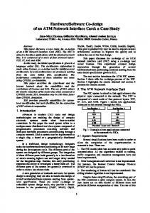
tral limit theorem is appropriate. However, when the profile reveals the quadratic approximation to be poor, there will be a marked discrepancy between the confidence intervals based on asymptotic normality and those based on the contours of the likelihood function. In such a case, the Wald intervals are prima facie suspect, because the Wald interval works by assuming a quadratic approximation to the likelihood surface, while the likelihood ratio method works directly with the likelihood surface. A. Ronald Gallant’s (1987, p. 147) advice on the matter is to “simply use the likelihood ratio statistic in preference to the Wald statistic.” McCullough (2003) examined a nonlinear least-squares model for which the profiles are not straight lines, and in a Monte Carlo analysis found that the likelihood intervals provided better coverage than the Wald intervals. For present purposes, profiling all 42 parameters is both extremely burdensome and unnecessary. The eigensystem analysis of the Hessian, presented in Table 3, indicates that the unit eigenvector associated with the largest normalized eigenvalue has an extremal component ⫺0.999986 in the direction of the parameter ␩. Therefore, we compute the likelihood profile of ␩, which has a value of 1.05071E-5 and a standard error of 6.265E-6. We use TSP to profile the likelihood. All profile estimations were produced by 100 iterations of BHHH followed by Newton iterations until convergence. The LogL on the signed square root scale is plotted against the studentized parameter in Figure 1(a), along with a dotted line with unit slope through the origin. The profile has a slight kink at the origin, with a slope of about unity to the right and a slope greater than unity to the left; this reveals a lack of symmetry in the likelihood. Farther from the origin, even a lack of linearity is evident, and the lack of monotonicity suggests the existence of multiple local optima. These conclusions are confirmed by examining the profile of LogL0 against ␩0 in Figure 1(b). At the other extreme, corresponding to the 40th and 42nd smallest eigenvalues are two eigenvectors with extremal elements of 0.668 and ⫺0.419, respectively, both in the direction of ␳, which has a value of 0.790645 and a standard error 0.154528. Examining Figure 2(a) at the origin, the profile is linear to the right but curved to the left. Further from the origin, a lack of linearity is pronounced, and it can be

VOL. 93 NO. 3


FIGURE 1. LIKELIHOOD PROFILES

seen that ␶0 ranges from ⫺2 to ⫹4, instead of a symmetric ⫺4 to ⫹4; this indicates skewness of the likelihood. These conclusions are confirmed by Figure 2(b), which presents the profile of LogL0 against ␳0 , the left side of which tends toward an asymptote. Thus, for both parameters the quadratic approximation is not valid. This implied asymmetry of the sampling distribution of the parameters suggests that likelihood-based intervals will be preferable to those based on asymptotic normality. Meeker and Escobar (1998) give several examples of likelihoodbased intervals. Additionally, bootstrap methods may also be useful in the presence of such asymmetry, as discussed in Vinod (2000b). We have little doubt that profiling other parameters would produce similar results. We conclude that the quadratic approximation cannot sustain confidence intervals based on normality. In part due to the inadequacy of the quadratic approximation, we do not present standard errors of the coefficients. Were we to produce confidence intervals for the parameters, we might use likelihood ratio intervals or the bootstrap. Regardless, we certainly would not

OF

885

␩

rely on the usual method. The other reason why we do not present standard errors is that we are skeptical of the validity of the parameter estimates themselves, as we show next. D. Additional Considerations While the gradient appears to be zero and the trace exhibits quadratic convergence, the Hessian is extremely ill-conditioned and negative semidefinite, and the likelihood profile suggests that the quadratic approximation is invalid. Taken together, these results leave us far from convinced that the TSP solution is valid, and there remains one more consideration on this point. We have argued elsewhere (McCullough and Vinod, 1999, p. 645) that “A user should always have some idea of the software’s precision and range, and whether his combination of algorithm and data will exhaust these limits.” The analysis thus far allows us to conclude that the SN problem does exhaust the limits of a PC. Specifically, given a 64-bit computing environment, i.e., PC computing, the 42-parameter

886


FIGURE 2. LIKELIHOOD PROFILES

problem posed by SN equation (13) satisfies Wright’s (1993) definition of a “large” optimization problem: “[A] ‘large’ problem is one in which the number of variables (or constraints) noticeably affects our ability to solve the problem in the given computing environment.” Notice the difference between the LogL values associated with the two solutions for which TSP declared convergence: 1967.071433588422 (储 g储 ⫽ 66.9) and 1967.071433588423 (储 g储 ⫽ 8.5E-9). They differ only in the twelfth decimal, i.e., the sixteenth significant digit, yet the gradient of one is decidedly nonzero, while the gradient of the other is zero.18 Considering the extreme ill-conditioning of 18

Note that both analytic first and second derivatives were employed. It is no wonder that approaches based on numerical derivatives met with little success. This does not constitute a call for the wholesale abandonment of numerical derivatives. Experience with the NIST StRD nonlinear least-squares problems suggests that for run-of-the-mill problems, and even some fairly hard ones, the difference between well-programmed numerical derivatives and analytical derivatives, especially when summed, is small enough that the former can give quite satisfactory solutions.

OF

JUNE 2003

␳

the Hessian, the prospective solution is located in a very flat region of the parameter space, so flat that the difference between the zero and nonzero gradient occurs in the sixteenth digit of the value of the likelihood. This sixteenth digit, almost assuredly, is corrupted by rounding error, so we really do not know what the value of LogL is at the maximum (assuming this point is a maximum). Thus, it can be seen that the problem posed by SN has completely exhausted the limits of PC computing, and more powerful computational methods will be needed to analyze this problem properly. We further observe that the use of analytic derivatives does not guarantee a solution, but they have enabled us to see that we do not have a solution: the SN problem, as posed, cannot be reliably solved on a PC. So far we have not presented standard errors for our coefficients for two reasons. First, if we do not trust the coefficients, we cannot possibly trust the standard errors. Second, even if we did trust the coefficients, we are not sure that the finite-sample properties of the likelihood will support asymptotic normal inference. In order

VOL. 93 NO. 3


TABLE 4—COMPARISON OF t-STATISTICS FOR SELECTED COEFFICIENTS Coefficient

␳ ␩ S

SN (BHHH) TSP (BHHH) TSP (Hessian) 4.1 2.6 1.6

5.1 1.7 1.8

6.6 2.8 2.3

to make a further point about standard errors in the context of nonlinear estimation, let us assume that the TSP solution is valid and that the quadratic approximation holds, and inquire into the significance of some important coefficients; for example, those discussed at length on pp. 541–542 of SN. SN, by using the GAUSS maxlik procedure at default, obtained BHHH standard errors; we convert their coefficients and standard errors to t-stats. For purposes of comparison, we present TSP BHHH t-stats from our TSP solution. Results are in Table 4. Notice how ␩ has gone from significant to insignificant. SN write (1999, p. 542), “The parameter ␩ is 0.15 and significant at the 1percent level. This implies that an increase of one million people (holding electoral votes and everything else constant) would lead to less effort which, in turn, would result in a 1-percent decrease in participation.” By contrast, the value of ␳ has increased dramatically, from 0.587 to 0.791, which would imply that the effect of the leader’s effort is even more pronounced. We note also that, had we used analytic Hessian standard errors, the t-stats for ␳, ␩, and S would have been 6.6, 2.8, and 2.3, respectively. This raises the age-old question of which standard error to use. See, e.g., Davidson and MacKinnon (1993, Secs. 8.6 and 13.5) or Greene (2000, Sec. 4.5.2). We merely wish to suggest that the researcher should not accept uncritically the default standard errors offered by the software. IV. On the Process of Replication

As part of our continuing investigation into the reliability of econometric software (McCullough and Vinod, 1999; McCullough, 2000b; Vinod, 2001), our original goal was to replicate each article in an issue of this journal using the author’s software package. Porting the code to other software packages might have enabled us

887

to determine the extent to which econometric results are software-dependent. Regrettably, we had to abandon the project because we found that the lesson of William G. Dewald et al. (1986) has not been well-learned: the results of much research cannot be replicated. Many authors do not even honor this journal’s replication policy, let alone ensure that their work is replicable. Gary King (1995, p. 445) posed the relevant questions: “[I]f the empirical basis for an article or book cannot be reproduced, of what use to the discipline are its conclusions? What purpose does an article like this serve?” We selected the June 1999 issue of this journal, and found ten articles that presented results from econometric/statistical software packages. Two of these were theory articles that did some computation—we deleted them from our sample to focus on empirical work. We began trying to collect data and code from authors as soon as the issue was out in print. Three authors supplied organized data sets and code. These three papers were primarily centered on linear regression. From a computational perspective, they are not fertile ground when one is searching for numerical difficulties; we did not bother to attempt replicating these papers.19 Though the policy of the AER requires that “Details of computations sufficient to permit replication must be provided,” we found that fully half of the authors would not honor the replication policy. Perhaps this should not be surprising—Susan Feigenbaum and David Levy (1993) have clearly elucidated the disincentives for researchers to participate in the replication of their work, and our experience buttresses their contentions. Two authors provided neither data nor code: in one case the author said he had already lost all the files; in another case, the author initially said it would be “next semester” before he would have time to honor our request, after which he ceased replying to our phone calls, e-mails, and letters. A third author, after several months and numerous requests, finally supplied us with six diskettes containing over 400 files—and no README file. Reminiscent 19

Even linear procedures must be viewed with caution. Giuseppe Bruno and Riccardo De Bonis (2003) gave the same panel data problem to three packages and got three different answers for the random-effects estimator. However, they traced all the discrepancies to legitimate algorithmic differences in the programs.

888


of the attorney who responds to a subpoena with truckloads of documents, we count this author as completely noncompliant. A fourth author provided us with numerous datafiles that would not run with his code. We exchanged several e-mails with the author as we attempted to ascertain how to use the data with the code. Initially, the author replied promptly, but soon the amount of time between our question and his response grew. Finally, the author informed us that we were taking up too much of his time—we had not even managed to organize a useable data set, let alone run his data with his code, let alone determine whether his data and code would replicate his published results. The final paper was by SN, who obviously honored the replication policy. This paper contained an extremely large nonlinear maximumlikelihood problem that greatly intrigued us, so we decided to examine it in detail. Thus, it became our case study. Professor Shachar cooperatively and promptly exchanged numerous e-mails with us as we sought to produce a useable data set and understand his code. Professor Nalebuff, too, was most helpful. They continued to assist us even after we declared that their nonlinear problem was too large for a PC.20 Replication is the cornerstone of science. Research that cannot be replicated is not science, and cannot be trusted either as part of the profession’s accumulated body of knowledge or as a basis for policy. Authors may think they have written perfect code for their bug-free software package and correctly transcribed each data point, but readers cannot safely assume that these error-prone activities have been executed flawlessly until the authors’ efforts have been independently verified. A researcher who does not openly allow independent verification of his results puts those results in the same class as the results of a researcher who does share his data and code but whose results cannot be replicated: the class of results that cannot be verified, i.e., the class of results that cannot be trusted. A researcher can claim that his results are correct 20

For the record, the SN paper contains 11 tables of results. We did not attempt to replicate Tables 1, 2, and 8 (which are Monte Carlo results), 10 (which contains the results of algebraic calculations), and 11. Excepting typographical errors, we had no difficulty replicating Tables 3, 4, 5, 6, and 7.

JUNE 2003

and replicable, but before these claims can be accepted they must be substantiated. This journal recognized as much when, in response to Dewald et al. (1986), it adopted the aforementioned replication policy. If journal editors want researchers and policy makers to believe that the articles they publish are credible, then those articles should be subject, at least in principle, to the type of verification that a replication policy affords. Therefore, having a replication policy makes sense, because a journal’s primary responsibility is to publish credible research, and the simple fact is that “research” that cannot be replicated lacks credibility. Many economics journals have similar replication policies: The Economic Record, Journal of International Economics (JIE), Journal of Human Resources, International Journal of Industrial Organization (IJIO), and Empirical Economics are but a few. Our own informal investigation suggests that the policy is not more effective at these journals than at the American Economic Review. We chose recent issues of JIE and IJIO, and made modest attempts to solicit the data and code: given the existence of the World Wide Web, we do not believe that obtaining the data and code should require much more effort than a few mouse clicks. We sent either e-mails or, if an e-mail address could not be obtained, a letter, to the first author of each empirical article, requesting data and code; for IJIO there were three such articles, and for JIE there were four. Only two of the seven authors sent us both data and code. There may be some problems with the implementation of replication policies at the above journals, but the problems certainly are remediable. What is difficult to believe is that 17 years after Dewald et al. (1986), most economics journals have no such policy, e.g., Journal of Political Economy, Review of Economics and Statistics, Journal of Financial Economics, Econometrica, Quarterly Journal of Economics, and others. One cannot help but wonder why these journals do not have replication policies. Even in the qualitative discipline of history, authors are expected to make available their data, as evidenced by the recent Bellesiles affair (James Lindgren, 2002). Our experience with the June 1999 issue of the AER is the first test of the AER policy of which we are aware, and the policy does not fare well. Obtaining data and code from authors

VOL. 93 NO. 3


after their paper is in print can be a formidable task. Even for the authors who sent data/code files, of which there were six, we had to wait anywhere from days to months for the author to supply the data and code. This, of course, was after we made successful contact with the author, a process that itself took anywhere from days to weeks. Sometimes the data were in a file format that could only be read by the author’s software, rather than in ASCII. Some of the code we received exhibited exceedingly poor programming style: unindented, uncommented, and generally undecipherable by anyone not intimately familiar with the package in question— here we recommend an excellent article by Jonathan Nagler (1995) on how to write good code for archival purposes. The code should be written and commented so as to guide a user who has a different software package. Ensuring that one’s work is replicable is no easy task, as Micah Altman and Michael P. McDonald (2003) demonstrated. As solutions to these problems, as part of a symposium on the topic of replication, King (1995) discussed both the replication standard, which requires that a third party could replicate the results without any additional information from the author, and the replication data set, which includes all information necessary to effect such a replication.21 Naturally, this includes the specific version of the software, as well as the specific version of the operating system. This should also include a copy of the output produced by the author’s combination of data/ code/software version/operating system. In the field of political science, many journals have required a replication data set as a condition of publication.22 Some economics journals have archives; often they are not mandatory or, as in the case of the Journal of Applied Econometrics, only data is mandatory, while code is optional. A “data-only” requirement is insuffi-

21 Some journals permit authors to “embargo” their data for a period of time, so that the author will have exclusive use of the data for that period. Of course, the empirical results of articles based on embargoed data cannot be trusted or used as the basis of policy-making, for those results cannot be replicated at least until the embargo ends. 22 American Journal of Political Science, Political Analysis, British Journal of Political Science, and Policy Studies Journal are but four.

889

cient, though, as Jeff Racine (2001) discovered when conducting a replication study. As shown by Dewald et al. (1986), researchers cannot be trusted to produce replicable research. We have shown that the replication policies designed to correct this problem do not work. The only prospect for ensuring that authors produce credible, replicable research is a mandatory data/code archive, and we can only hope that more journals recognize this fact. To the best of our knowledge the only economics journals that have such a policy are the Federal Reserve Bank of St. Louis Review, the Journal of Money, Credit, and Banking, and Macroeconomic Dynamics. The cost of maintaining such an archive is low: it is a simple matter to upload code and (copyright permitting) data to a web site.23 The benefits of an archive are great. First, there would be more replication (Richard G. Anderson and Dewald, 1994). Second, as we recently argued (McCullough and Vinod, 1999, p. 661), more replication would lead to better software, since more bugs would be uncovered. Researchers wishing to avoid software-dependent results will take Stokes’ (2003) advice and use more than one package to solve their problems; this will also lead to more bugs being uncovered. Finally, the quality of research would improve: knowing that eager assistant professors and hungry graduate students will scour their data and code looking for errors, prospective authors would spend more time ensuring the accuracy, reliability, and replicability of their reported results. V. Conclusions

The textbook paradigm ignores computational reality by accepting uncritically the output from a computer program’s nonlinear estimation procedure. Researchers generally follow this paradigm when publishing in economics journals, even though it is well known that nonlinear solvers can produce incorrect answers. We advocate a four-step process whereby a proposed solution can be verified. We illustrate our method by making a case 23 In the case of proprietary data, the researcher should provide some information on the data that does not violate the copyright, e.g., the mean of each series, so that another researcher who obtains the data from the proprietary source can be sure he is using the exact same data.

890


study of one nonlinear estimation from a recently published article by Shachar and Nalebuff (1999). The four-step process not only can be used to verify a possible solution, it can also assist in determining whether a problem is too large for the computer at hand. Indeed, this proved to be the case with the Shachar/Nalebuff nonlinear maximum likelihood problem. Finally, we have vindicated our previous assertion concerning replication policies, that such “policies are honored more often in the breach” (McCullough and Vinod, 1999, p. 661). Mere “policies” do not work, and only mandatory data/ code archives can hope to achieve the goal of replicable research in the economic science. Computational Details: For TSP v4.5 r 06/07/01 (as well as “R” v1.5.0, in which graphics were rendered) and Mathematics v4.1 the operating system was Linux v2.2.18 (Red Hat v7.1) on a 733 MHz Pentium III. GAUSS v3.5 was run on 733 MHz Pentium III under Windows Millenium Edition. REFERENCES Albert, A. and Anderson, J. “On the Existence of

Maximum Likelihood Estimations in Logistic Regression Models.” Biometrika, April 1984, 71(1), pp. 1–10. Altman, Micah and McDonald, Michael P. “Replication with Attention to Numerical Accuracy.” Political Analysis, 2003 (forthcoming). Anderson, Richard G. and Dewald, William G.

“Replication and Scientific Standards in Applied Economics a Decade After the Journal of Money, Credit, and Banking Project.” Federal Reserve Bank of St. Louis Review, November/December 1994, 76(6), pp. 79 – 83. Bates, Douglas and Watts, Donald G. “A Relative Offset Orthogonality Convergence Criterion for Nonlinear Least Squares.” Technometrics, May 1981, 23(2), pp. 179 – 83. . Nonlinear regression analysis and its applications. New York: J. Wiley and Sons, 1988. Berndt, Ernst; Hall, Robert; Hall, Bronwyn and Hausman, Jerry. “Estimation and Inference in

Nonlinear Structural Models.” Annals of Economic and Social Measurement, October 1974, (3/4), pp. 653– 65. Bischof, C. H.; Bu¨cker, H. M. and Lang, B. “Automatic Differentiation for Computational Fi-

JUNE 2003

nance,” in E. J. Kontoghiorghes, B. Rustem, and S. Siokos, eds., Computational methods in decision-making, economics and finance, volume 74 of applied optimization. Dordrecht: Kluwer Academic Publishers, 2002, pp. 297–310. Box, George E. P. and Jenkins, Gwilym M. Time series analysis: Forecasting and control. San Francisco: Holden-Day, 1976. Box, George E. P. and Tiao, George C. Bayesian inference in statistical analysis. Reading, MA: Addison-Wesley, 1973. Brooks, Chris; Burke, Simon P. and Persand, Gita. “Benchmarks and the Accuracy of

GARCH Model Estimation.” International Journal of Forecasting, January 2001, 17(1), pp. 45–56. Bruno, Giuseppe and De Bonis, Riccardo. “A Comparative Study of Alternative Econometric Packages with an Application to Italian Deposit Interest Rates.” Journal of Economic and Social Measurement, 2003 (forthcoming). Datta, Biswa N. Numerical linear algebra and applications. New York: Wiley, 1995. Davidson, Russell and MacKinnon, James G. Estimation and inference in econometrics. New York: Oxford University Press, 1993. . Econometric theory and methods. New York: Oxford University Press, 2003. Dennis, J. E. and Schnabel, Robert B. Numerical methods for unconstrained optimization. Philadelphia, PA: SIAM Press, 1996. Dewald, William G.; Thursby, Jerry G. and Anderson, Richard G. “Replication in Empir-

ical Economics: Journal of Money, Credit, and Banking Project.” American Economic Review, September 1986, 76(4), pp. 587– 603. Doornik, Jurgen and Ooms, Marius. “Multimodality and the GARCH Likelihood.” Working paper, Nuffield College, Oxford, 2000. Feigenbaum, Susan and Levy, David. “The Market for (Ir)Reproducible Econometrics.” Social Epistemology, 1993, 7(3), pp. 215–32. Fiorentini, Gabrielle; Calzolari, Giorgio and Panattoni, Lorenzo. “Analytic Derivatives and the

Computation of GARCH Estimates.” Journal of Applied Econometrics, July–August 1996, 11(4), pp. 399 – 417. Gallant, A. Ronald. Nonlinear statistical models. New York: J. Wiley and Sons, 1987. Gill, Philip E.; Murray, Walter and Wright, Margaret H. Practical optimization. New York:

Academic Press, 1981.

VOL. 93 NO. 3


Golub, Gene H. and van Loan, Charles F. Matrix

computations, 3rd edition. Baltimore, MD: Johns Hopkins University Press, 1996. Greene, William. Econometric analysis, 4th edition. Saddle River, NJ: Prentice-Hall, 2000. Hauck, Walter W. and Donner, Allan. “Wald’s Test as Applied to Hypotheses in Logit Analysis.” Journal of the American Statistical Association, December 1977, 72(360), pp. 851– 53. Judd, Kenneth. Numerical methods in economics. Cambridge, MA: MIT Press, 1998. Kaiser, J. “Software Glitch Threw Off Mortality Estimates.” Science, June 14, 2002, 296, pp. 1945– 47. King, Gary. “Replication, Replication.” Political Science & Politics, September 1995, 28(3), pp. 444 –52. Lindgren, James. “Fall From Grace: Arming America and the Bellesiles Scandal.” Yale Law Journal, June 2002, 111(8), pp. 2195– 249. Maddala, G. S. Introduction to econometrics, 2nd edition. New York: MacMillan, 1992. McCullough, B. D. “Assessing the Reliability of Statistical Software: Part II.” American Statistician, May 1999a, 53(2), pp. 149 –59. . “Econometric Software Reliability: EViews, LIMDEP, SHAZAM and TSP.” Journal of Applied Econometrics, March/ April 1999b, 14(2), pp. 191–202; “Comment” and “Reply,” January/February 2000, 15(1), pp. 107–11. . “Experience with the StRD: Application and Interpretation,” in K. Berk and M. Pourahmadi, eds., Proceedings of the 31st symposium on the interface: Models, prediction and computing. Fairfax, VA: Interface Foundation of North America, 2000a, pp. 15–21. . “Is It Safe to Assume That Software Is Accurate?” International Journal of Forecasting, July/September 2000b, 16(3), pp. 349 –57. . “Some Details of Nonlinear Estimation,” in M. Altman, J. Gill, and M. McDonald, eds., Numerical methods in statistical computing for the social sciences. New York: J. Wiley and Sons, 2003. McCullough, B. D. and Renfro, Charles G.

“Benchmarks and Software Standards: A Case Study of GARCH Procedures.” Journal of Economic and Social Measurement, 1999, 25(2), pp. 59 –71.

891

. “Some Numerical Aspects of Nonlinear Estimation.” Journal of Economic and Social Measurement, 2000, 26(1), pp. 63–77. McCullough, B. D. and Vinod, H. D. “The Numerical Reliability of Econometric Software.” Journal of Economic Literature, June 1999, 37(2), pp. 633– 65. McCullough, B. D. and Wilson, Berry. “On the Accuracy of Statistical Procedures in Microsoft Excel 97.” Computational Statistics and Data Analysis, July 1999, 31(1), pp. 27– 37. . “On the Accuracy of Statistical Procedures in Microsoft Excel 2000 and Excel XP.” Computational Statistics and Data Analysis, December 2002, 40(4), pp. 713–21. Meeker, William Q. and Escobar, Luis A. “Teaching about Approximate Confidence Regions Based on Maximum Likelihood Estimations.” American Statistician, February 1995, 49(1), pp. 48 –53. . Statistical methods for reliability data. New York: J. Wiley and Sons, 1998. Mittelhammer, Ron C.; Judge, George G. and Miller, Douglas J. Econometric foundation.

New York: Cambridge University Press, 2000. Nagler, Jonathan. “Coding Style and Good Computing Practices.” Political Science & Politics, September 1995, pp. 488 –92. Nerlove, Marc. “Chapter One: The Likelihood Principle.” Unpublished manuscript, University of Maryland, 1999. Newbold, Paul; Agiakloglou, Christos and Miller, John. “Adventures with ARIMA Software.”

International Journal of Forecasting, December 1994, 10(4), pp. 573– 81. Nocedal, Jorge and Wright, Stephen J. Numerical optimization. New York: Springer, 1999. Overton, Michael. Numerical computing with IEEE floating point arithmetic. Philadelphia, PA: SIAM, 2001. Racine, Jeff. “On the Nonlinear Predictability of Stock Returns Using Financial and Economic Variables.” Journal of Business and Economic Statistics, July 2001, 19(3), pp. 380 – 82. Rao, C. R. Linear statistical inference and its applications. New York: J. Wiley and Sons, 1973. Revkin, Andrew. “Data Revised on Soot in Air and Deaths.” New York Times (National Edition) June 5, 2002, p. A23. Ritter, Christian and Bates, Douglas M. “Profile

892


Methods,” in A. Prat, ed., Compstat 96. Heidelberg: Physica, 1996, pp. 123–34. Rose, Colin and Smith, Murray. Mathematical statistics with Mathematica. New York: Springer, 2002. Schoenberg, Ron. “Optimization with the Quasi-Newton Method.” Unpublished manuscript, Aptech Systems, Maple Valley, WA, 2001. Seber, G. A. F. and Wild, C. J. Nonlinear regression. New York: J. Wiley and Sons, 1989. Shachar, Roni and Nalebuff, Barry. “Follow the Leader: Theory and Evidence on Political Participation.” American Economic Review, June 1999, 89(3), pp. 525– 47. Stokes, Houston. “On the Advantage of Using Two or More Econometric Software Systems to Solve the Same Problem.” Journal of Economic and Social Measurement, 2003 (forthcoming). Ueberhuber, Christoph W. Numerical computation, volume 1. New York: Springer, 1997a. . Numerical computation, volume 2. New York: Springer, 1997b.

JUNE 2003

Venables, W. N. and Ripley, B. D. Modern ap-

plied statistics with S-plus, 3rd edition. New York: Springer, 1999. Vinod, H. D. “Review of Gauss for Windows, Including Its Numerical Accuracy.” Journal of Applied Econometrics, March/April 2000a, 15(2), pp. 211–20. . “Foundations of Multivariate Inference Using Modern Computers.” Linear algebra and its applications, December 2000b, 321(1/3), pp. 365– 85. . “Care and Feeding of Reproducible Econometrics.” Journal of Econometrics, January 2001, 100(1), pp. 87– 88. Vinod, H. D. and Ullah, Aman. Recent advances in regression methods. New York: MarcelDekker, 1981. Wolfram, Stephen. The mathematica book, 4th edition. New York: Cambridge University Press, 1999. Wright, Margaret H. “Some Linear Algebra Issues in Large-Scale Optimization,” in Marc S. Moonen, Gene H. Golub, and Bart L. R. de Moor, eds., Linear algebra for large-scale and real-time applications. Dordrecht: Kluwer Academic Publishers, 1993, pp. 315–37.

Verifying the Solution from a Nonlinear Solver: A Case Study - CiteSeerX

Verifying the Solution from a Nonlinear Solver: A Case Study - CiteSeerX

Suggest Documents

Verifying the Solution from a Nonlinear Solver: A Case ... - CiteSeerX

Verifying a Signature Architecture â A Comparative Case Study

Verifying a Signature Architecture â A Comparative Case Study

A Case Study from Computer Science - CiteSeerX

A Case Study - CiteSeerX

A Case Study - CiteSeerX

A Case Study - CiteSeerX

A Case Study - CiteSeerX

a case study - CiteSeerX

a Case Study - CiteSeerX

a case study - CiteSeerX

the wam case study: verifying compiler correctness for ... - CiteSeerX

the wam case study: verifying compiler correctness for ... - CiteSeerX

A Nonperiodic, Nonlinear Eulerian Gyrokinetic Solver for ... - CiteSeerX

A Case Study of Verifying and Validating an ...

A Case Study of Verifying and Validating an Astrophysical Simulation ...

A Case Study of Verifying and Validating an ...

Analyzing Alloy Constraints using an SMT Solver: A Case Study

A case study from paleoecology

A Case Study from Chile

A Case Study from Qatar

a case study from Niger

results from a case study in the geometry domain - CiteSeerX

A case study on the path from academic practices - CiteSeerX

Verifying the Solution from a Nonlinear Solver: A Case Study - CiteSeerX