Vertical Forecasting of Temperature, Dissolved

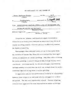
Journal of Environmental Science and Engineering A 3 (2014) 87-105 Formerly part of Journal of Environmental Science and Engineering, ISSN 1934-8932

D

DAVID

PUBLISHING

Vertical Forecasting of Temperature, Dissolved Oxygen, pH and Conductivity in the Amadorio Reservoir by Multivariate Methods Jorge Bluhm Gutiérrez1, Alicia Esparza Martínez2, Ernesto Patricio Nuñez Peña1, Felipe de Jesús Escalona Alcázar1, Santiago Valle Rodríguez1 and Josefina Huerta García3 1. Academic Unit of Earth Sciences, University Autonomous of Zacatecas, Zacatecas 98058, México 2. Academic Unit of Culture, University Autonomous of Zacatecas, Zacatecas 98058, México 3. Academic Unit of Biological Sciences, University Autonomous of Zacatecas, Zacatecas 98058, México Received: August 07, 2014 / Accepted: August 21, 2014 / Published: September 20, 2014. Abstract: PCA (principal component analysis), CCA (canonical correlation analysis) and PLSR (partial least squares regression) are powerful water quality modeling methods that provide better results than other classical ones such as multiple lineal regression. In this work they were used to model four water quality parameters at the Amadorio Reservoir (Alicante, Spain), namely: water temperature, dissolved oxygen, pH and conductivity. The main purpose of this study was to predict the future quality of the water and, thus improve its management. Raw data correspond to daily values of mean wind speed, mean wind direction, maximum wind speed, mean, minimum and maximum air temperature, number of hours below 7 ºC, relative humidity, global solar radiation, total precipitation, evapotranspiration, exploitation volume, inflow, outflow, filtration, depth and Julian day. Two years were considered (2004-2005) to get the calibration (186 days, 4,401 registrations) and validation (185 days, 4,573 registrations) datasets. Models were developed using either all the variables or a reduced subset; furthermore, PLSR yielded the best results. Key words: Water quality management, canonical correlation analysis, partial least squares.

1. Introduction Water quality is one of the most important characteristics to be assessed when managing aquatic resources [1]. Particularly, in the Mediterranean regions, reservoirs are probably the most important and unique, big bodies of fresh water for human activities [2]. Quite frequently, natural sources that feed water to reservoirs lack the quality required for its different uses. Therefore, observations on the site in real time are necessary to ensure water quality [3]. In the Amadorio Reservoir (Alicante, Spain), this is carried through a multiparametric probe, installed in 2003 to Corresponding author: Jorge Bluhm Gutiérrez, doctor, research field: water resources. E-mail: [email protected].

measure temperature, dissolved oxygen, pH and conductivity at different depths with the aim of elaborating vertical profiles of these constituents. One-dimensional modeling continues to be an effective and useful approach to describe water quality [4]. Multivariate approaches are gaining acceptance and revealing their usefulness [5-9]. There is an introduction of the three multivariate statistical techniques (with references to more particular details for interested readers) and, to finalize the main objectives of this work are summarized. Water temperature can be considered the most important variable in any aquatic system because it affects numerous water quality parameters and determines the presence and development of living organisms [10]. Also, the thermal stratification

88

Vertical Forecasting of Temperature, Dissolved Oxygen, pH and Conductivity in the Amadorio Reservoir by Multivariate Methods

regulates chemical and biological processes that take place in a reservoir, determining its water quality, as well as that of the river flowing downstream [11]. Oxygen is another important factor in lakes and reservoirs [4] as it controls many chemical oxidation reactions and can be used as a parameter indicative of the general condition of the aquatic system [12]. Biota is highly sensitive to extreme pH values; however, there is an existing range for each organism allowing it to live optimally [13]. Furthermore, some chemical substances in the reservoir’s sediment can dissolve back to water because of extreme pH values, as it is the case with some heavy metals [14]. Conductivity can be used in water analysis to estimate the content of dissolved and suspended solids. It is a general measure of water quality and constitutes a basic parameter to evaluate its adequacy for different uses, such as irrigation [15]. The meteorological parameters and the reservoir state variables are of upmost importance in the monitoring of water quality and they will be discussed in the experimental section. Multivariate methods constitute a useful tool in research studies implying large datasets [16]. One of the relevant advantages is that they do not require previous knowledge on the samples or the variables. The objective of this work is to predict temperature, dissolved oxygen, pH and conductivity through the application of multivariate techniques: PCA (principal component analysis), CCA (canonical correlation analysis) and PLSR (partial least squares regression).

2. Calculation and Methods 2.1 The Amadorio Reservoir The Amadorio Reservoir is located in the Province of Alicante (Spain) and includes the Algar River and the Amadorio River basins (Fig. 1). Its coordinates in UTM (Universal Transverse Mercator) 30 are X: 738,390 m-Y: 4,272,435 m. The reservoir basin surface is 205 km2, with an annual mean contribution of 6 hm3, the longitude of the main river-bed is 30 km

and the mean slope of the river-bed is 3.43%, its benchmark in regards to the mean level of the sea is of 127.00 m. It has a spillway type Creager with floodgates, bottom drainage, and two outlets: an inferior outlet in the right riverbank and a superior outlet in the left riverbank. The reservoir is used for irrigation and as water supplier for Benidorm City and Villajoyosa City (Fig. 1). Its total capacity is 16.00 hm3 and it belongs to the so-called Marina Baja Exploitation System, which was classified as high risk because it belongs to a geographical zone with frequent droughts. The climate of the area is semi-arid Mediterranean with a mean temperature of 16 ºC, and a mean rainfall of 360 mm. 2.2 Experimental Data 2.2.1 Multiparametric Probe In 2003, an automatic multiparametric probe was installed close to the Outlet Works of the Amadorio Reservoir to continuously monitor the physic-chemical characteristics of the water reservoir. The multiparametric probe was installed in a fixed unit that was mounted near to the Amadorio Outlet Works, so that it is representative of the water for treatment. The probe measures four signal parameters at different depths (temperature, dissolved oxygen, pH and conductivity, some depths ranging from 0.42 m to 30.00 m), which allow the establishment of vertical and temporary profiles for each analytical parameter. Further, the dataset obtained by the multiparametric probe is suitable to carry out traditional one-dimensional modeling and to manage and predict the quality of the water in the reservoir [3, 17]. Data from 2004 showed values outside the current experimental ranges (more likely because of wrong measurements, functional problems, etc.), in all cases the input data were removed. In 2005, those problems were avoided and no record was deleted. In 2004, 138 days had complete records, whereas, in 2005, 233 days were recorded. Hence, data values were completed for 371 valid days. They were divided into two subsets,

Vertical Forecasting of Temperature, Dissolved Oxygen, pH and Conductivity in the Amadorio Reservoir by Multivariate Methods

Fig. 1

89

Localization map of the Amadorio Reservoir.

one for modeling (186 days, 4,401 records) and one for validation (185 days, 4,573 registrations). The descriptive statistics of the variables for each dataset were studied to verify that the experimental ranges agreed [10]. 2.2.2 Weather Conditions The weather parameters are important to assess the water quality. Therefore, climatological data from the Villajoyosa Weather Station were used to register daily-average values for: wind mean speed (V, km·h-1); wind mean direction (DV, º); wind maximum speed (Vx, km·h-1); mean temperature (T, ºC); minimum air temperature (Tn, ºC); maximum air temperature (Tx, ºC); number of hours below 7 ºC (Hf); mean relative humidity of the air (HR, %); global solar radiation (Rad, W·m-2); total precipitation (P, mm); and reference evapotranspiration (ETo, mm). 2.2.3 Variables of State The variables of state of the reservoir were: volume of exploitation (VolExp, m3); reservoir inflow (Qent,

m3·day-1); reservoir outflow (Qsal, m3·day-1); filtration (Filt, m3·day-1); and depth (Profundidad, m). Additionally, the Julian day variable was considered to introduce a periodic component in the analysis. This variable is initially used to determine if the season affected the quality of water through mechanisms not covered with other variables that were used. 2.3 Chemometric Methods All chemometric studies were carried out with Excel, SPSS 15.0 for Windows, and Statgraphics Centurion XV. 2.3.1 Classical One-Dimensional Modelling Modeling water quality reservoirs has been traditionally performed by univariate methods, like multiple linear regression [5, 10, 18]. Çamdevýren et al. [5] used the relationships between Chlorophyll-a and 16 chemical variables. Physical and biological water quality variables in

90

Vertical Forecasting of Temperature, Dissolved Oxygen, pH and Conductivity in the Amadorio Reservoir by Multivariate Methods

Çamlidere reservoir (Ankara, Turkey) were studied by using PCS (principal component scores) in MLR (multiple linear regression analysis) to predict Chlorophyll-a levels. Two approaches were used. In the first approach, only five selected score values obtained by PCA (principal components analysis) were used for the prediction of Chlorophyll-a levels and predictive success (R2) of the model found it to be 56.3%. In the second approach, all score values obtained from the PCA were used as independent variables; the predictive power was turned out to be 90.8%. Deas and Lowney [10] looked into past decades and dozens of modelling efforts which ranged from simple statistical relationships to complex dynamic models that have been applied to rivers and reservoirs. They point out that the empirical models are statistical relationships between two or more observed characteristics of a particular system. 2.3.2 PCA PCA aims to reduce the original dimensionality of data so that, from p experimental original variables, knew abstract variables are obtained as the linear combination of the p variables [19]. Typically k is selected to be much lower than p; however, there is a restriction that the original data, with as much information as possible, should be explained with a reduced number of principal components. PCA was used with the purpose of achieving several objectives: to revise the homogeneity hypothesis for the calibration and validation periods [20], to detect if some variables show tendency behaviors on the whole, and to purify the information eliminating the erroneous data [16, 21]. 2.3.3 CCA The purpose of a canonical analysis is to characterize the independent statistical relationships that exist between two (and possibly more) sets of random variables [22]. CCA allows the establishment of the interrelations that may exist between two groups of variables. This is done by identifying the

linear combinations of the variables of the first group that are most correlated with some linear combinations of the variables of the second group. Hence, it can be easily seen that this technique degenerates to the multiple regression technique when one of the groups is reduced to a single variable [23]. The variables are divided into two groups so that a group of variables in one group may be used to predict the variables of the other group [16]. In general, this is accomplished by establishing a linear combination between the predictive variables and the response variables [19]. The CCA allows an explicit partition of a group of data given in explanatory variables and response variables, with the purpose of identifying vector couples in these partial spaces of data [24]. A comprehensive explanation of CCA and technical details can be found elsewhere [19, 22, 25-26]. Some CCA applications at reservoirs are shown in Refs. [27-30]. 2.3.4 PLSR PLSR is a multivariate calibration technique that sets a relationship among a group of predictive data, termed X-block, and a group of responses, Y-block. PLSR was demonstrated to be capable of providing stable predictions even when X contains highly correlated variables [31] and some noise [32]. PLSR relates the predictive variables and the response variables by means of inner linear regression models developed between the so-called latent variables (which, similarly to the principal components, are linear combinations of the original variables) [32]. The prediction capabilities of the models can be improved by adjusting the number of latent variables included into the model [33]. There are numerous applications of the methodology in main fields within analytical chemistry, as well as comprehensive explanations on the algorithms [6, 20, 34-38]. Singh et al. [31] analyzed a surface water quality data set pertaining to a polluted river using PLSR models.

Vertical Forecasting of Temperature, Dissolved Oxygen, pH and Conductivity in the Amadorio Reservoir by Multivariate Methods

3. Results 3.1 Classic Method The classic method for water quality modeling at reservoirs is the mechanicist model. The reservoir is modeled as a group of horizontal layers, in the vertical direction and one-dimensional form (Fig. 2). Many of the big reservoirs are stratified and have appreciable temperature vertical gradients and other constituents; however, they are laterally uniformed. The variation main axis for water storages is vertical [39]. Each layer is considered as uniform in its thermal attributes and the layer parameters are assigned in its half point [12]. Mixing process and water quality in reservoirs are controlled by natural variations in inflows, outflows, and meteorological forcings. In man-made reservoirs, of course, the mixing is also controlled to a large degree by the manner in which they are regulated [39]. This type of modeling was conducted by Bluhm [40]

Fig. 2

Horizontally layered model of the reservoir.

91

for the Ta (water temperature) variable using the same data of the Amadorio Reservoir for the calibration and validation periods, obtaining for the validation period R2 = 0.915 of explained variability, with an estimate standard error of 2.01 °C. The variables that are nearest to their minimum and maximum values in the periods of calibration and validation are: V, DV, Vx, T, Tn, Tx, HR, Rad, ETo, VolExp, Qsal, Profundidad, Ta and Odis. On the other hand, those that show a smaller coincidence of the minimum and maximum values for the calibration data and validation data are: DJ, Hf, P, Qent, Filt, pH and Con. 3.2 Data Structure and Anomalous Data Detection When applying the PCA, the data were previously standardized with the purpose of eliminating the influence of the different measure units and to homogenize the dimensionality of the data. This technique was used in the periods of calibration and

92

Vertical Forecasting of Temperature, Dissolved Oxygen, pH and Conductivity in the Amadorio Reservoir by Multivariate Methods

validation using the total of the predictive variables and response variables. For the calibration group, five outstanding principal components were obtained. That explains 75.9% of the total variability (Table 1). To compare the explained variability in the validation group, five components were obtained and these represent 75.1% of the variance (Table 2). To be able to detect anomalous data, the dispersion Table 1

diagrams of the components were used in pairs. Small groups of points can be appreciated in some of the diagrams very far from the rest, like in the dispersion diagram of the components 5 and 6 (calibration group, Fig. 3). The weights in the first five components for the calibration and validation periods are shown in Table 3.

Variance percentage explained by the components with eigenvalue greater than the unit, calibration group. Principal components analysis

Component number

Eigenvalue

Variance percentage

Storage percentage

1

6.79448

32.355

32.355

2

3.16844

15.088

47.442

3

2.73154

13.007

60.450

4

2.12718

10.129

70.579

5

1.11699

5.319

75.898

Table 2

Variance percentage explained by the first five components, validation group. Principal components analysis

Component number

Eigenvalue

Variance percentage

Storage percentage

1

7.06814

33.658

33.658

2

3.10922

14.806

48.464

3

2.61874

12.470

60.934

4

1.71601

8.171

69.105

5

1.26001

6.000

75.105

Fig. 3

Dispersion diagram of the components 5 and 6, calibration group.

Vertical Forecasting of Temperature, Dissolved Oxygen, pH and Conductivity in the Amadorio Reservoir by Multivariate Methods Table 3

93

Weights in the first five principal components, calibration and validation periods.

Variable 1

2

Calibration

Validation

Components

Components

3

4

5

1

2

3

4

5

DJ

0.1307

0.3734

-0.0712

0.3329

-0.0159

0.3252

-0.1020

0.0614

-0.2068

-0.1154

V

-0.0500

-0.2619

0.2659

0.4160

0.1355

-0.0155

0.1171

-0.5014

-0.3220

0.1277

DV

-0.2210

0.0642

0.0130

0.2466

-0.2430

-0.0868

-0.0709

-0.0321

-0.0588

-0.5141

Vx

-0.0250

-0.1621

0.1999

0.4320

0.4572

-0.0486

0.0614

-0.3739

-0.4084

0.3726

T

0.3714

0.0253

-0.0268

0.0116

0.0658

0.3498

0.0579

0.0123

0.0331

0.0163

Tn

0.3678

0.0554

-0.0417

0.0036

0.0566

0.3453

0.0284

0.0586

0.0064

0.0544

Tx

0.3669

0.0101

-0.0275

0.0028

0.0390

0.3435

0.0709

-0.0222

0.0348

-0.0058

Hf

-0.1932

-0.2568

0.1367

-0.1090

-0.3962

-0.2029

-0.1208

-0.1227

-0.2020

-0.0884

HR

0.0180

0.2474

-0.2600

-0.4352

0.1399

-0.0107

-0.1746

0.4753

0.0744

0.1472

Rad

0.2907

-0.2584

0.1318

-0.1101

0.0014

0.1668

0.2807

-0.2279

0.3703

-0.0886

-0.0637

0.2295

-0.1138

0.0058

0.2574

-0.0344

-0.1171

0.2185

-0.2251

0.4023

ETo

0.3346

-0.2010

0.1231

-0.0008

0.0760

0.2573

0.2448

-0.2611

0.2081

-0.0025

VolExp

0.0836

-0.4026

0.0880

-0.3464

0.1776

-0.2438

0.2283

-0.0729

0.3702

0.2272

P

Qent

-0.2217

0.1179

-0.0612

-0.0306

0.4070

-0.2999

-0.0841

-0.0601

-0.0791

-0.1907

Qsal

0.2808

0.2058

-0.0703

0.2167

-0.2509

0.3203

-0.0543

0.0281

-0.1395

-0.0088

Filt

-0.1254

0.0587

-0.0045

0.0517

-0.1195

-0.0717

-0.0105

-0.1354

-0.0511

-0.4690

0.0134

0.1706

0.4381

-0.2082

0.1684

0.0141

-0.3814

-0.2302

0.3718

0.1836

Profundidad Ta

0.2792

-0.0734

-0.3053

0.1673

-0.1008

0.1849

0.3315

0.2254

-0.3075

-0.1300

Odis

-0.2244

-0.2546

-0.3618

0.0913

-0.0041

-0.2484

0.3365

0.1067

-0.0539

-0.0146

pH

-0.0602

-0.0950

-0.4096

0.0463

0.3712

-0.1734

0.3196

0.1718

0.0430

0.0391

Con

-0.0470

0.3750

0.3858

-0.0532

0.0704

0.0684

-0.4768

-0.1359

0.0228

-0.0665

3.3 Canonical Correlation Analysis

T, Tn, Tx, Hf, HR, ETO, VolExp, Qsal and Profundidad. The results of the adjustment are shown in Table 5.

3.3.1 Using 17 Predictive Variables At the beginning, the variables were standardized for all the analyses made with CCA. The variables were standardized using the values corresponding to the mean and standard deviation of the calibration group. The results in the validation period are shown in Table 4. 3.3.2 Using Nine Predictive Variables To fulfill the parsimony principle, that is, to simplify the model without losing prediction power, the number of variables was decreased. In this way, the variables were selected inside the first two canonical

variables

(those

that

explain

more

variability), the weights of the independent variables with numeric value higher than 0.10 were selected. There were nine variables included with this approach:

3.4 PLSR In all the method applications used in this study, the X and Y variables were standardized before starting[41]; this helps eliminate the fraction of data that is common in all registrations [42, 43]. Besides that, the data adjustment is increased [44]. The algorithm PLS1 will be applied in all cases, that is, the response variables Y predicted individually (only one at a time) [45]. Each application will be proven with different number of components and the quantity allowing the best prediction in the validation period will be used to model most of the systematic variability [43]. Also, some specific variants existing in the PLSR will be developed with the purpose of improving the estimate.

94

Vertical Forecasting of Temperature, Dissolved Oxygen, pH and Conductivity in the Amadorio Reservoir by Multivariate Methods

Table 4 Results of predictions of the CCA in the validation period, using 17 predictive variables, standardized with the parameters of the calibration period. Variable

Q2 corrected

Ta

0.679

4.07

Typical error of the estimation

Odis

0.682

2.62

pH

0.434

0.44

Con

0.604

74.95

Table 5 Results of predictions of the CCA applied in the validation period, using nine predictive variables, standardized with the parameters of the calibration period. Variable

Q2 corrected

Typical error of the estimation

Ta

0.657

4.13

Odis

0.738

2.58

pH

0.475

0.44

Con

0.607

77.97

3.4.1 Using 17 Predictive Variables The results obtained by using 17 predictive variables for the validation period are shown in Table 6. The number of components extracted is indicated to model each variable, which is different for each response variable. 3.4.2 Evaluating the Julian Day Effect The Julian day variable was represented to evaluate if the season effect in the response variables is already considered; however, in the remaining predictive variables, the PLSR was applied without including this variable Julian day. The results of the modeling using 16 predictive variables for the validation group are shown in Table 7. Due to the obtained results, the variable Julian day in the following analyses will not be used. 3.4.3 Trimming the Data Several steps were taken: first, the data were ordered by variable. Then data bigger than 99% and smaller than 1% were replaced for the values of these limits [42]. The trimming was applied to the predictive and response variables. The trimming process was only applied to the calibration group. The results are shown in Table 8. 3.4.4 Model Reduced in Linear Terms To fulfill the parsimony principle, the variables with significant standardized coefficients were

selected from the PLSR graphs for each water quality variable used. The procedure to select the appropriate variables to model each one consisted on proving models that included different numbers of predictive variables, until an expression that explained practically the same quantity of variability that the complete model with 16 variables but only using some of them (for example, the standardized coefficients for dissolved oxygen show this concept, Fig. 4) was gotten. The regression characteristics are pointed out in Table 9. 3.4.5 Extended Matrix of Entrances With the objective of improving the regression, the matrix of entrances can extend including non-linear terms of the predictive variables X (logarithms, quadratic values, cubic values, reciprocal values) and later development of the linear PLSR is developed on that extended matrix [35] for each water quality variable. This variant of the PLSR is denominated INLR (implicit to non-linear PLS regression) and it has been shown that it allows the modeling of non-soft linearities (of second or third polynomial degree) in the relationships X-Y [46]. The obtained values are shown in Table 10. 3.4.6 Non-linear Regression Non-linear models were analyzed considering each

Vertical Forecasting of Temperature, Dissolved Oxygen, pH and Conductivity in the Amadorio Reservoir by Multivariate Methods

95

Table 6 Results of predictions with the PLSR using 17 predictive variables to predict the response variables, algorithm PLS1, validation period. Period

Variable

Extracted components

Ta Validation

R2

Estimation error

7

0.697

4.02

Odis

14

0.686

2.61

pH

11

0.434

0.44

Con

8

0.608

72.36

Table 7 Results of predictions with the PLSR using 16 predictive variables, discarding the Julian day variable, algorithm PLS1, validation group. Period

Variable

Extracted components

Ta Validation

R2

Estimation error

7

0.675

4.04

Odis

14

0.741

2.59

pH

12

0.476

0.44

Con

12

0.606

78.76

Table 8 Results of predictions with the PLSR using 16 predictive variables that were applied trimmed, algorithm PLS1, validation period. Period

Variable

Extracted components

Ta Validation

R2

Estimation error

4

0.694

4.03

Odis

13

0.742

2.61

pH

10

0.472

0.43

Con

8

0.610

77.86

Fig. 4 Table 9 terms.

Profundidad

Qsal Filt

VolExp Qent

P

ETo

Rad

Tx Hf HR

T

Tn

Vx

V DV

Odis

Standardized coefficients of the PLSR model, using 16 predictive variables for dissolved oxygen. Results of predictions with the PLSR applied to the period of validation, algorithm PLS1, models reduced in linear

Period

Validation

Variable

Number of predictive variables

Extracted components

R2

Estimation error

Ta

5

2

0.689

4.07

Odis

4

3

0.749

2.32

pH

6

6

0.484

0.42

Con

3

3

0.630

71.44

96

Vertical Forecasting of Temperature, Dissolved Oxygen, pH and Conductivity in the Amadorio Reservoir by Multivariate Methods

Table 10 Results of predictions with the PLSR applied to the validation period, algorithm PLS1, using the extended matrix of entrances. Period

Validation

Variable

Number of used terms

Extracted components

R2

Estimation error

Ta

7

6

0.695

4.04

Odis

6

5

0.719

2.71

pH

7

4

0.472

0.41

Con

4

4

0.639

73.57

Table 11 Results of predictions with the PLSR applied to the validation period, algorithm PLS1, nonlinear regression, using the results of the reduced model in linear terms. Period

Validation

Variable

R2

Ta

0.743

3.54

Odis

0.755

2.38

pH

0.484

0.42

Con

0.631

71.48

of the four variables of water quality, like independent variable, X, which estimates the value of water quality and dependent variable, Y, with observed values. Linear, quadratic, cubic, logarithmic, compound, growth, S curve, exponential, inverse, power and logistics regressions were proven. In each case, the regression accepted was that which presented a bigger coefficient of determination, R2. The value parameters that measure the adjustment from the observations are shown in Table 11.

4. Discussion 4.1 Initial Study of the Data The revision of the minimum and maximum values that the variables take in the calibration and validation periods undoubtedly leave on one hand that the great majority of predictive variables values present in the calibration period are also in the validation period. These are V, DV, Vx, T, Tn, Tx, HR, Rad, ETo, VolExp, Qsal and Profundidad; therefore, these variables are good options which can be included in the regression expressions. On the other hand, the predictive variables that present more similar variation ranges in the two periods are Ta and Odis, hoping their predictions will be better than pH and Con variables. The first five principal components for calibration and validation show (Tables 1 and 2), through the

Estimation error

variability explained individually and as a whole (75.9% and 75.1%, respectively), that the global behavior of the predictive and response variables is practically uniform, opening the possibility of making inferences, and using models obtained in the calibration group to carry out predictions for the validation group. The PCA performance to locate very outstanding anomalous data showed great effectiveness when using the components diagrams for pairs. For example, Fig. 3 shows some anomalous data. Several of these anomalous data refer to the balance calculated data in the storage and this is possibly due to certain phenomenas, such as the occurrence of intense rains or openings of floodgates which require the use of intervals larger than 24 h. When revising weights for the first five components in the calibration and validation groups (Table 3), the calibration for the first component explains 32.4% of the variance and the variables that possess bigger weights in this component are: T, Tn,, Tx, Rad, ETo, Qsal and Ta; it is possible to interpret that this component represents the thermal energy and its balance in the system. For the validation group, the first component explains 33.7% of the variance and the variables with more weight in this component are: DJ, T, Tn, Tx, ETo, Qent and Qsal; it is observed that

Vertical Forecasting of Temperature, Dissolved Oxygen, pH and Conductivity in the Amadorio Reservoir by Multivariate Methods

some changes exist in the formation of the component, mainly when including DJ because it is introduced in the component as a bound factor to the date of the year (temporary factor). That diminished their weight Rad and Ta and the volume of entrances Qent increased their influence, impacting this component. The prediction capacity of a model can be explained by the fact that the loads of the first principal component or factor in the calibration and test samples are very similar for both groups. A good part of the variation in the test group can be explained by the first principal component [47]. The second component for the calibration group represents 15.1% of the variance and the most important variables are: DJ, V, Hf, VolExp, Odis and Con; this component can interpret the wind speed variation through the season of the year, the hours of cold temperature, and the exploitation volume in the reservoir and their influence in dissolved oxygen and conductivity. In the validation group, the second component explains 14.8% of the variability and the variables that saturate this component are: Rad, Profundidad, Ta, Odis, pH and Con; this component includes the influence of the radiation and mainly of the depth in the four variables of water quality. The third component for the calibration period contains 13.0% of the group total variance and this component is more influenced by the variables HR, Profundidad, pH and again Ta, Odis and Con; therefore, the variation of relative humidity and, mainly, of depth, and how they influence the four variables of water quality is manifested. In the validation group, the third component represents 12.5% of the variance and the variables that influence it are: V, Vx, HR and ETo; there is a combined variation of the mean speed and maximum speed of the wind, of the relative humidity, and the evapotranspiration. The variables that saturate this component in a more important way differ considerably for the two periods. The fourth component in the calibration group

97

explains 10.1% of the total variability and the variables that impacts more are: V, Vx, and HR; therefore, it is representing the variation of the mean speed and maximum speed of the wind along with relative humidity. In the validation group, the fourth component constitutes 8.2% of the variance and the variables with more weight are: Vx, Rad, VolExp, Profundidad and Ta; it is a component influenced mainly by the maximum speed of the wind, radiation, volume of the storage and depth, which impacts the temperature of the water. The only variable in common in the formation of the component in the two periods is Vx. The fifth component in the period of calibration explains a 5.3% variability and the variables that influence this component are: Vx, Hf, P, Qent, Qsal and pH; this component picks up the importance of maximum speed air, the hours of cold temperature, precipitation, volumes that enter and leave the reservoir and how these variables influence the pH. For the validation group, the fifth component contains 6.0% of the variance and the variables that have bigger weight in the component are: DV, Vx, P and Filt; here the combined manifestation of the wind direction, their maximum speed of the day, the precipitation, and the filtration can be appreciated. In this case, the fifth component in the validation does not include any of the response variables. The first component is the most important because it explains a bigger variance quantity and the most influential variables are practically the same ones, however,

the

other

components

show

bigger

variability within the variables that appear with more weight. 4.2 CCA Results It is important to point out that the standardization variables as predictive or as response allow that the results obtained with the CCA improve. Also, the parameters for the standardization (the mean and the standard deviation) are very important because they

Vertical Forecasting of Temperature, Dissolved Oxygen, pH and Conductivity in the Amadorio Reservoir by Multivariate Methods

98

influence the predictions. To standardize the predictive variables, in the calibration group and in the validation group, the mean and the standard deviation obtained for the variables in the calibration were used. When using 17 predictive variables, the results of Table 4 were obtained, the best variable explained is dissolved oxygen (R2 = 0.682) followed by water temperature (R2 = 0.679). Continuing in the prediction quality comes conductivity (R2 = 0.604) and the pH variable ended with a smaller determination coefficient (R2 = 0.434). Table 5 shows the prediction results for nine predictive variables. When comparing the analysis carried out with the 17 and with the nine predictive variables, it is observed that the water temperature diminishes very little its determination coefficient (R2 = 0.657) and increases its estimate error very weakly (4.13 ºC) when passing from 17 to nine variables; however, the determination coefficients of the dissolved oxygen (R2 = 0.738, the one that more Table 12

increased), the pH (R2 = 0.475), and the conductivity (R2 = 0.607) improve. Additionally, the estimate errors decrease for the dissolved oxygen (2.58 mg·L-1) and the pH (0.44) and the estimate error for the conductivity (77.97 S·cm-1) increases a little. Therefore, the analysis with nine variables is globally better than the one carried out with 17, thus the simplification of the model is achieved without global loss of prediction power. For the water temperature variable, the best prediction utilizing CCA was to use 17 predictor variables (R2 = 0.679 and standard estimation error of 4.07 °C), however, in the mechanistic conventional method by horizontal layers predictive power was better (R2 = 0.915 and standard estimation error of 2.01 °C). The correlation analysis carried out with nine predictive variables has the characteristics that are shown in Table 12 and the coefficients of the canonical variables can be seen in Table 13.

Canonical correlation analysis with nine predictive variables standardized.

Number

Eigenvalue

Canonical correlation

Wilks lambda

1

0.878535

0.937302

2

0.698269

3

0.426065

4

0.213395

Table 13

Chi-Cuadrado

p-value

0.016546

18,018.40

0.0000

0.835625

0.136220

8,757.38

0.0000

0.652736

0.451461

3,493.61

0.0000

0.461947

0.786605

1,054.45

0.0000

Coefficients for the canonical variables of the first and the second series, using nine predictive variables. U2

U3

ZT

0.8873

-0.2296

-0.3012

0.2977

ZTn

-0.0299

0.4189

-0.1996

-0.9486

ZTx

-0.5369

0.1561

0.5468

0.9606

ZHf

-0.0158

0.2700

-0.1421

-0.9854

ZHR

0.1669

-0.1042

-0.1713

0.0673

ZETo

0.5220

-0.0156

-0.5841

-1.0830

-0.3454

0.2882

1.2927

0.6990

0.2406

0.1500

0.4320

0.0816

Canonical variable

ZVolExp ZQsal ZProfundidad Canonical variable ZTa

U1

0.2528 V1 0.6937

-0.8718 V2

0.3456

U4

-0.2206

V3

V4

0.5198

-1.1529

-0.0149

ZOdis

-0.6970

0.3921

-1.4021

-0.3501

ZpH

0.1439

-0.4033

0.2260

1.1760

ZCon

0.2340

-0.5691

-1.6176

0.0391

99

V1

Vertical Forecasting of Temperature, Dissolved Oxygen, pH and Conductivity in the Amadorio Reservoir by Multivariate Methods

U1 Fig. 5

Graph of the first couple of canonical variables, using nine standardized predictive variables.

The first couple’s graph of canonical variables sample shows that the relationship among them is approximately linear (Fig. 5). The p-values are next to zero, which confirms the hypothesis that the two blocks of variables are related to each other. The biggest canonical correlation has a value of 0.94 explaining a 0.88 / (0.88 + 0.70 + 0.43 + 0.21) = 40% of the variability and represents the relationship between the variable T and ETo (thermal energy in the environment), that influences the canonical variable U1, and the relationship between Ta and Odis (with contrary signs) which possess bigger weight in V1; this indicates that for more thermal energy in the atmosphere, there is bigger temperature in water and smaller dissolved oxygen. The second canonical correlation has a value of 0.84 that represents 31% of variability and includes the relationship between the Profundidad variable and the conductivity so, and revising the reservoir profile in a given day, it was observed that for a greater depth corresponds a greater conductivity. The third correlation is 0.65 which includes 19% of the variance of the group and manifests the relationship between the VolExp variable and the conductivity. This manner will diminish all levels of conductivity when increasing the stored volume. The fourth correlation has a value of 0.46, capturing a percentage of

variability of 10%, where the influence of some of the predictive variables is manifested on the pH variable. 4.3 PLSR Results When 17 predictive variables are used (Table 6), the variable better simulated is the water temperature (R2 = 0.697) using seven components only; followed by the dissolved oxygen that has a determination coefficient similar to the previous one (R2 = 0.686) but 14 components were extracted; the explained variability of the conductivity continues in descending order (R2 = 0.608) and eight components were obtained; the variable with the lowest determination coefficient (R2 = 0.434) is the pH, calculated with 11 components. The determination coefficient was higher and the error was reduced for all the variables when the PLSR was used instead of the CCA, except for the pH which showed identical couple of values in the two methods. This can be due to the pH, being the response variable with smaller variation range and whose value modifies a little [32, 33, 43, 48]. When the Julian day was not used as a predictive variable, with the purpose of evaluating the effect of their absence, the algorithm PLS1 was applied for each response variable using 16 predictive variables (Table 7) and it was observed that the water temperature lightly diminished its explained

100

Vertical Forecasting of Temperature, Dissolved Oxygen, pH and Conductivity in the Amadorio Reservoir by Multivariate Methods

variability (R2 = 0.675) and almost maintained its estimate error similar to when 17 variables were used (4.04 ºC); the dissolved oxygen significantly increased its determination coefficient (R2 = 0.741) and slightly diminished its error (2.59 mg·L-1); the pH also increased its explained variability (R2 = 0.476) and conserved its estimate error equally (0.44); last the conductivity practically maintained its R2 with the same value (0.606) and its error of estimate increased lightly (78.76 S·cm-1). When making a global balance, it is more convenient not to consider the Julian day variable in the analysis, with that, the global adjustment has a similar quality. The trimmed data made on 16 variables (Table 8) improved the explained variability of the water temperature (R2 = 0.694) and slightly diminished their prediction error (4.03 ºC); the dissolved oxygen practically conserved its same values of explained variability and error (R2 = 0.742 and 2.61 mg·L-1); with the pH (R2 = 0.472 and 0.43 of error) and the 2

-1

conductivity (R = 0.610 and 77.86 S·cm ), the same thing happened, varying its quantities very little. It was observed that when applying the trimming of data, the best results in the PLSR were obtained using fewer components for each response variable in comparison to the application of the same technique when the data were not trimmed. This process implies additional calculations, as it is observed that the advances are reduced for this case. The fact that the adjustment parameters are practically the same can be an indicative that the atypical values absence not modifies the regression process considerably. It is possible because with the PCA they were eliminated completely. The results of using in the regressions less variables (approach of the reduced model in linear terms) expressed in Table 9 show that in comparison with the model with 16 variables, the reduced model improvement in all aspects, with the exception of the error in the water temperature estimate. The coefficient determination of water temperature with

the reduced model improved a little (R2 = 0.689) and the error increased slightly (4.07 ºC); the dissolved oxygen was explained better (R2 = 0.749) and the error diminished substantially (2.32 mg·L-1); the variability of the pH was represented better (R2 = 0.484) and its error diminished (0.42); the conductivity improved its determination coefficient (R2 = 0.630) and it diminished the estimate error substantially (71.44 S·cm-1). Therefore, the pattern reduced in linear terms provides a superior adjustment for the data. For each response variable, the number of extracted factors has decreased enough; this fact possibly explains the improvement in the regression because the eliminating factors contribute little information and a lot of noise. The graph of dissolved oxygen observations and predictions considering the model reduced in linear terms is shown in Fig. 6. Also, the expressions to estimate the variables of water quality are simpler than those 16 variables: Ta _ Est  8.32020.310551Profundidad    n (1) 0.000112235Q sal 0.56017ETo 0.191481T 0.180964T

Odis _ Est 11.12680.752148ETo 0.342047Profundidad0.238237Tx



 8.68778x10

7

(2)

Vol

Exp

pH _ Est 7.431430.144645ETo





0.0305618Tx 0.0259479Tn  1.11747x10 7 VolExp 0.0408722Hf 0.0154395Profundidad

(3) Con _ Est 1220.888.71871Profundidad   0.0000336155VolExp 0.854586ETo

(4)

The termination _Est in Eqs. (1) and (4) mean estimate values. By including the PLSR in the non-linear regression terms of the predictive variables (extended matrix of entrances), it is expected for it to deal with a lack of possible linearity in the relationship among variables. The results for the most significant terms for each response are shown in Table 10. When comparing

Vertical Forecasting of Temperature, Dissolved Oxygen, pH and Conductivity in the Amadorio Reservoir by Multivariate Methods

Fig. 6

101

Graphs of observations and predictions, considering the PLSR model reduced in linear terms, for dissolved oxygen.

with the obtained results of the models outlined with linear terms (Table 9), the explained variability of the water temperature lightly increases (R2 = 0.695) and the estimate error slightly diminishes (4.04 ºC); the determination coefficient of the dissolved oxygen falls sensibly (R2 = 0.719) and its estimate error increases (2.71 mg·L-1); the pH diminished its explanation percentage (R2 = 0.472) and its error was almost the same (0.41); the conductivity slightly increased its explained variability (R2 = 0.639) and its estimate error increased (73.57 S·cm-1). Also, the number of terms used to obtain the estimate of the response variables is bigger, in all cases, than the terms used in the models reduced in linear terms. Therefore, due to the similarity of the quality of results, it is observed that the models in linear terms are better because their expressions are simpler. On the other hand, when making nonlinear regressions on the estimates made with the linear reduced model and the observed values of variables in water quality and after proving several types of regressions for each of the response variables, the best results are shown in Table 11, and when comparing them with the models reduced in linear terms (Table 9), the water temperature is the only variable that improved enough its modeling because increasing

the explained variability (R2 = 0.743) and its error diminishment (3.54 ºC); while the dissolved oxygen increased its determination coefficient (R2 = 0.755) and its estimate error (2.38 mg·L-1); the pH remained the same in its explained variability (R2 = 0.484) and error (0.42); the conductivity practically continued the same (R2 = 0.631 and error of 71.48 S·cm-1). Therefore, the only non-linear regression to take into account will be the one made for the water temperature that is shown in Fig. 7. The expressions obtained for each one of the response variables are the following: Ta 11.231604 0.060883 Ta _ Est  0.020614 Ta _ Est  0.00223407 Ta _ Est  2

3

(5)

O dis 

11.915435/ 154.990249exp  0.659802O dis _ Est  

(6) pH0.0695477 1.017231 pH _ Est  0.00106663 pH _Est 

2

(7)

Con 21.609260





1.042232 Con _ Est  2.05126x10 5  Con _ Est 

2

(8)

Vertical Forecasting of Temperature, Dissolved Oxygen, pH and Conductivity in the Amadorio Reservoir by Multivariate Methods

Ta_Observed

102

Ta_Estimated Fig. 7 Graph of observations and predictions for the water temperature, when making the cubic regression on the linear reduced model and the observations.

For the water temperature prediction in the validation period using the PLSR, it was better to do non-linear regression on the estimated values with the linear reduced model and the observed values and testing various regressions types (R2 = 0.743 and estimation standard error 3.54 °C). However, the classical mechanistic method of horizontal layers had greater predictive power for water temperature (R2 = 0.915 and estimation standard error 2.01 °C).

5. Conclusions An example was presented to examine the efficiency of two multivariate statistical methods: the CCA and the PLSR, to predict profiles of four variables of reservoir water quality: temperature, dissolved oxygen, pH and conductivity. The available data included groupings of days (not consecutive) in the Amadorio Reservoir (Spain) and consisted of information of the state’s reservoir, meteorological data of the nearest station (Villajoyosa Station), and

data in the 2004 and 2005 vertical profiles of the water quality variables. The available data were divided into two groups (calibration and validation) and descriptive statistics were used to check its homogeneity. The PCA was applied to detect anomalous data using the scores of the registrations in diagrams for the components by pairs; the similarity of the two periods that grouped the data was also verified through the study of variable weights in the components. The CCA allowed establishing relationships between the block of predictive variables and the block of response variables; standardizing the data of the validation group using the values corresponding to the mean and the standard deviation of the calibration data. Also, the CCA allowed discovering clear relationships between some predictive variables and the response variables using the canonical variables coefficients and its correlations. The CCA allowed the making of predictions of water quality variable values in the period of validation, by using some of predictive

Vertical Forecasting of Temperature, Dissolved Oxygen, pH and Conductivity in the Amadorio Reservoir by Multivariate Methods

variables. The PLSR was applied to obtain better regressions through some of its variants: reduction of the number of predictive variables to use only the most significant, trimmed data, and extended matrix entrances (INLR). It was observed that the selection of number factors with better results can be obtained of the explanation of bigger parts of the systematic variability [43] and to introduce less noise in the analysis. Also, this procedure imposes since the beginning fewer restrictions than other chemometric methods and it is possible to make it on significant variables, selected from the diagrams of standardized coefficients. The PLSR in order to provide appropriate results should be applied under the Homogeneity Principle, which implies that the effects of the state and meteorological variables do not change substantially through time; implying certain continuity under the conditions of its tributaries and that new contamination sources contributions will not take place in the basin. In the made regressions, the best results were obtained with this method. Also, the PLSR allowed knowing which predictive variables possess bigger influence on the water quality variables analyzed in this work.

References [1]

[2]

[3]

[4]

[5]

Armengol, J. 2000. Analysis and Evaluation of Reservoirs as Ecosystems. Barcelona: Universidad de Barcelona. Rueda, F., Moreno-Ostos, E., and Armengol, J. 2006. “The Residence Time of River Water in Reservoirs.” Ecological Modelling 191 (2): 260-74. Prats i Vime, R., and Correcher Martínez, E. 2004. “Continuous Monitoring of the Quality of the Water in Reservoir.” Presented at Working Group 24, VII National Congress of the Environment. Accessed January 20, 2013. http://www.conama.org/documentos/ GT24.pdf. Antonopoulos, Z. V., and Gianniou, K. S. 2003. “Simulation of Water Temperature and Dissolved Oxygen Distribution in Lake Vegoritis, Greece.” Ecological Modelling 160 (1-2): 39-53. Çamdevýren, H., Demýr, N., Kanik, A., and Keskýn, S. 2005. “Use of Principal Component Sscores in Multiple

[6]

[7]

[8]

[9]

[10]

[11]

[12]

[13] [14]

[15] [16] [17]

[18]

103

Linear Regression Models for Prediction of Chlorophyll-a in Reservoirs.” Ecological Modelling 181 (4): 581-9. Einax, W. J., Aulinger, A., Tümpling, V. W., and Prange, A. 1999. “Quantitative Description of Element Concentrations in Longitudinal River Profiles by Multiway PLS Models.” Fresenius Journal of Analytical Chemistry 363 (7): 655-61. Giussani, B., Dossi, C., Monticelli, D., Pozzi, A., and Recchia, S. 2006. “A Chemometric Approach to the Investigation of Major and Minor Ion Chemistry in Lake Como (Lombardia, Northern Italy).” Annali di Chimica 96 (5-6): 1-8. Shrestha, S., and Kazama, F. 2007. “Assessment of Surface Water Quality Using Multivariate Statistical Techniques: A Case Study of the Fuji River Basin, Japan.” Environmental Modelling & Software 22 (4): 464-75. Singh, P. K., Malik, A., Mohan, D., and Sinha, S. 2004. “Multivariate Statistical Techniques for the Evaluation of Spatial and Temporal Variations in Water Quality of Gomti River (India)—A Case Study.” Water Research 38 (18): 3980-92. Deas, L. M., and Lowney, L. C. 2000. Water Temperature Modelling Review. Central Valley: The Bay Delta Modeling Forum. Dolz, J., Puertas, J., Aguado, A., and Agulló, L. 1995. Thermal Effects in Dams and Reservoirs. Catalonia: Polytechnic University of Catalonia. Environmental Laboratory. 1995. CE-QUAL-R1: A Numerical One-Dimensional Model of Reservoir Water Quality; User’s Manual, Instruction Report E-82-1 (Revised Edition). US Army Engineer Waterways Experiment Station, Vicksburg. Manahan, E. A. 2000. Environmental Chemistry. Boca Raton: Lewis Publishers. Markiegi, X., Rallo, A., and Andía, A. 1999. Water Quality Protection in Zadorra System Reservoirs. Basque Country: Ararteko. Romero Rojas, A. J. 1999. Water Quality. Mexico: Alfaomega. Johnson, E. D. 2000. Multivariate Methods Applied to Data Analysis. Mexico: International Thomson Editores. Joehnk, D. K., and Umlauf, L. 2001. “Modelling the Metalimnetic Oxygen Minimum in a Medium Sized Alpine Lake.” Ecological Modelling 136 (1): 67-80. Gnauck, A. 2006. Water Quality Modelling and Management of Freshwater Ecosystems. Brandenburg:

104

Vertical Forecasting of Temperature, Dissolved Oxygen, pH and Conductivity in the Amadorio Reservoir by Multivariate Methods

Brandenburg University of Technology at Cottbus. [19] Pérez López, C. 2005. Advanced Statistical Methods with SPSS. Madrid: International Thomson Editores Spain Paraninfo S. A. [20] Wold, S., Sjöström, M., and Eriksson, L. 2001. “PLS-Regression: A Basic Tool of Chemometrics.” Chemometrics and Intelligent Laboratory Systems 58 (2): 109-30. [21] Martens, H., and Næs, T. 1989. Multivariate Calibration. New York: John Wiley & Sons. [22] Kettenring, R. J. 2006. Canonical Analysis. Encyclopedia of Statistical Sciences. New Jersey: John Wiley & Sons Inc. [23] Ouarda, J. M. B. T., Girard, C., Cavadias, S. G., and Bobée, B. 2001. “Regional Flood Frequency Estimation with Canonical Correlation Analysis.” Journal of Hydrology 254 (1-4): 157-73. [24] Callies, U. 2005. “Interaction Structures Analysed from Water-Quality Data.” Ecological Modelling 187 (4): 475-90. [25] Gutiérrez, M. J., Cano, R., Cofiño, S. A., and Sordo, M. C. 2004. Neural and Probabilistic Networks in the Atmospheric Sciences. Santander: Ministerio de Medio Ambiente. [26] Peña, D. 2002. Analysis of Multivariate Data. Madrid: McGraw-Hill/Inter-American of Spain. [27] Ariyadej, C., Tansakul, R., Tansakul, P., and Angsupanich, S. 2004. “Phytoplankton Diversity and Its Relationships to the Physico-Chemical Environment in the Banglang Reservoir, Yala Province.” Journal of Environmental Science and Technology 26 (5): 595-607. [28] McIninch, P. S., and Garman, C. G. 2000. Identification and Analysis of Aquatic and Riparian Habitat Impairment Associated with Dams of the Virginia Tide Water Region. Report to Virginia Department of Conservation & Recreation. Richmond. [29] Qingyun, Y., Yuhe, Y., Weisong, F., Zhigang, Y., and Hongtao, C. 2008. “Plankton Community Composition in the Three Gorges Reservoir Region Revealed by PCR-DGGE and Its Relationships with Environmental Factors.” Journal of Environmental Sciences 20 (6): 732-8. [30] Schallenberg, M., and Burns, W. C. 2003. “A Temperature, Tidal Lake-Wetland Complex. Water Quality and Implications for Zooplankton Community Structure.” New Zealand Journal of Marine and Freshwater Research 37: 429-47.

[31] Singh, P. K., Malik, A., Basant, N., and Saxena, P. 2007. “Multi-way Partial Least Squares Modelling of Water Quality Data.” Analytica Chimica Acta 584 (2): 385-96. [32] Baffi, G., Martin, B. E., and Morris, J. A. 1999. “Non-linear Projection to Latent Structures Revisited (the Neural Network PLS Algorithm).” Computers & Chemical Engineering 23 (9): 395-411. [33] Li, C., and Huang, H. 2003. “Model Building by Merging Submodels Using PLSR.” Journal of Chemical Engineering of Japan 36 (9): 1023-33. [34] Burnham, A. J., MacGregor, F. J., and Viveros, R. 2001. “Interpretation of Regression Coefficients under a Latent Variable Regression Model.” Journal of Chemometrics 15 (4): 265-84. [35] Li, C., Ye, H., Wang, G., and Zhang, J. 2005. “A Recursive Nonlinear PLS Algorithm for Adaptive Nonlinear Process Modelling.” Chemical Engineering and Technology 28 (2): 141-52. [36] Martens, H. 2001. “Reliable and Relevant Modelling of Real World Data: A Personal Account of the Development of PLS Regression.” Chemometrics and Intelligent Laboratory Systems 58 (2): 85-95. [37] Sundberg, R. 2006. “Small-Sample and Selection Bias Effects in Multivariate Calibration, Exemplified for OLS and PLS Regressions.” Chemometrics and Intelligent Laboratory Systems 84 (1-2): 21-5. [38] Wold, S., Trygg, J., Berglund, A., and Antti, H. 2001. “Some Recent Developments in PLS Modeling.” Chemometrics and Intelligent Laboratory Systems 58 (2): 131-50. [39] Martin, L. J., and McCutcheon, C. S. 1999. Hydrodynamics and Transport for Water Quality Modelling. Boca Raton: Lewis Publishers. [40] Bluhm, J. 2008. “One-Dimensional Modeling of Water Quality in Reservoirs. Comparative Analysis of Mechanistic and Multivariate Models.” Ph.D. thesis, Polytechnic University of Valencia. [41] Dayal, S. B., and MacGregor, F. J. 1997. “Improved PLS Algorithms.” Journal of Chemometrics 11 (1): 73-85. [42] Kettaneh, N., Berglund, A., and Wold, S. 2005. “PCA and PLS with Very Large Data Sets.” Computational Statistics & Data Analysis 48 (1): 69-85. [43] Ferré, J. 2006. Multivariate Calibration in Quantitative Analysis. The Inverse Model. Tarragona: Publica S. A. [44] Bro, R., and Smilde, K. A. 2003. “Centering and Scaling in Component Analysis.” Journal of Chemometrics 17 (1): 16-33. [45] Ergon, R. 2006. “Reduced PCR/PLSR Models by

Vertical Forecasting of Temperature, Dissolved Oxygen, pH and Conductivity in the Amadorio Reservoir by Multivariate Methods Subspace Projections.” Chemometrics and Intelligent Laboratory Systems 81 (1): 68-73. [46] Berglund, A., Kettaneh, N., Uppgård, L. L., Wold, S., Bendwell, N., and Cameron, R. D. 2001. “The GIFI Approach to Non-linear PLS Modelling.” Journal of Chemometrics 15 (4): 321-36. [47] Rodrigues, J., Alves, A., Pereira, H., Da Silva Perez, D., Chantre, G., and Schwanninger, M. 2006. “NIR PLSR

105

Results Obtained by Calibration with Noisy, Low-Precision Referente Values: Are the Results Aceptable?” Holzforschung 60 (4): 402-8. [48] Blanco, M., Coello, J., Iturriaga, H., Maspoch, S., and Redón, M. 1995. “Partial Least-Squares Regression for Multicomponent Kinetic Determinations in Linear and Non-linear Systems.” Analytica Chimica Acta 303 (2-3): 309-20.