Vessel-Diameter Quantification and Embolus Detection in CTA Images

Vessel-Diameter Quantification and Embolus Detection in CTA Images

Henri Bouma

The front cover shows a surface rendering of contrast-enhanced blood in pulmonary vessels. The shape of a healthy vessel-surface is convex, but at the location of an embolus – which is a clot inside the vessels – it is concave, because the blood is flowing around the clot. Isophote curvature is used to color the concave surface red. The back cover shows surface renderings of pulmonary vessels at several scales and thresholds. The top image shows the coarse shape of blood vessels at a high scale. The bottom image shows details of contrast-enhanced blood inside the vessels at a low scale.

c 2008 by H. Bouma, unless stated otherwise on chapter front pages, all rights Copyright reserved. No part of this publication may be reproduced by print, photocopy or any other means without the permission of the copyright owner. ISBN 978-90-386-1209-6 A catalogue record is available from the Eindhoven University of Technology Library. Printed by PrintPartners Ipskamp, The Netherlands. The work described in this thesis was performed at the Technische Universiteit Eindhoven in collaboration with Philips Medical Systems in Best. The CT data of patients with PE was provided by the Academic Medical Center in Amsterdam. The CT data of the cerebrovascular phantom was provided by the University Medical Center in Utrecht.

This work was carried out in the ASCI graduate school. ASCI dissertation series number 160.

Vessel-Diameter Quantification and Embolus Detection in CTA Images

PROEFSCHRIFT

ter verkrijging van de graad van doctor aan de Technische Universiteit Eindhoven, op gezag van de Rector Magnificus, prof.dr.ir. C.J. van Duijn, voor een commissie aangewezen door het College voor Promoties in het openbaar te verdedigen op woensdag 2 april 2008 om 16.00 uur

door

Henri Bouma

geboren te Uithuizermeeden

Dit proefschrift is goedgekeurd door de promotoren: prof.dr.ir. F.A. Gerritsen en prof.dr.ir. B.M. ter Haar Romeny Copromotor: dr. A. Vilanova i Bartrol´ı

Contents

1 Introduction 1.1 Vessel-Diameter Quantification . . . . . . . . . . . . . . . . . . . . . 1.2 Embolus Detection . . . . . . . . . . . . . . . . . . . . . . . . . . . . 1.3 Outline of the Thesis . . . . . . . . . . . . . . . . . . . . . . . . . . .

I

Vessel-Diameter Quantification

9 9 10 16

17

2 Gaussian Derivatives on Anisotropic Data 2.1 Introduction . . . . . . . . . . . . . . . . . . 2.2 Anisotropic Blurring . . . . . . . . . . . . . 2.3 Anisotropic Voxels . . . . . . . . . . . . . . 2.4 Experiments and Results . . . . . . . . . . . 2.5 Conclusions . . . . . . . . . . . . . . . . . .

. . . . .

. . . . .

. . . . .

. . . . .

. . . . .

. . . . .

. . . . .

. . . . .

. . . . .

. . . . .

. . . . .

. . . . .

. . . . .

. . . . .

19 20 21 24 26 27

3 Gaussian Derivatives based 3.1 Introduction . . . . . . . . 3.2 Accuracy of Methods . . . 3.3 Computational Cost . . . 3.4 Conclusions . . . . . . . .

. . . .

. . . .

. . . .

. . . .

. . . .

. . . .

. . . .

. . . .

. . . .

. . . .

. . . .

. . . .

. . . .

. . . .

29 30 32 36 40

4 Correction for the Dislocation of Curved Edges 4.1 Introduction . . . . . . . . . . . . . . . . . . . . . 4.2 Existing Edge-Detection Methods . . . . . . . . . 4.3 Analysis of Curved Edges and Surfaces . . . . . . 4.4 Approximation for Curved Surfaces in 3D . . . . 4.5 Implementation . . . . . . . . . . . . . . . . . . . 4.6 Experiments and Results . . . . . . . . . . . . . . 4.7 Conclusion . . . . . . . . . . . . . . . . . . . . .

. . . . . . .

. . . . . . .

. . . . . . .

. . . . . . .

. . . . . . .

. . . . . . .

. . . . . . .

. . . . . . .

. . . . . . .

. . . . . . .

. . . . . . .

41 42 42 43 49 49 50 57

on . . . . . . . .

B-Splines . . . . . . . . . . . . . . . . . . . . . . . . . . . .

. . . .

5 Unbiased Vessel-Diameter Quantification based 5.1 Introduction . . . . . . . . . . . . . . . . . . . . . 5.2 Method . . . . . . . . . . . . . . . . . . . . . . . 5.3 Experiments and Results . . . . . . . . . . . . . . 5.4 Conclusions . . . . . . . . . . . . . . . . . . . . .

II

on . . . . . . . .

FWHM . . . . . . . . . . . . . . . . . . . . . . . .

. . . .

. . . .

. . . .

Embolus Detection

6 Pulmonary Vessel Segmentation 6.1 Introduction . . . . . . . . . . . 6.2 Vessel Segmentation . . . . . . 6.3 Candidate Detection . . . . . . 6.4 Experiments and Results . . . . 6.5 Conclusions . . . . . . . . . . .

59 60 60 67 69

71 and . . . . . . . . . . . . . . .

PE Candidate Detection . . . . . . . . . . . . . . . . . . . . . . . . . . . . . . . . . . . . . . . . . . . . . . . . . . . . . . . . . . . . . . . . . . . . . . . . . . . . . . . . . . . . .

7 Features for Pulmonary-Embolus Classification 7.1 Introduction . . . . . . . . . . . . . . . . . . . . . 7.2 Features for PE Classification . . . . . . . . . . . 7.3 Experiments and Results . . . . . . . . . . . . . . 7.4 Conclusions . . . . . . . . . . . . . . . . . . . . . 8 Classification of Pulmonary-Embolus 8.1 Introduction . . . . . . . . . . . . . . 8.2 Training and Testing . . . . . . . . . 8.3 Evaluation of the CAD System . . . 8.4 Conclusions . . . . . . . . . . . . . .

. . . . .

73 74 75 80 81 86

. . . .

. . . .

. . . .

. . . .

. . . .

. . . .

. . . .

. . . .

. . . .

. . . .

87 . 88 . 89 . 98 . 102

Candidates . . . . . . . . . . . . . . . . . . . . . . . . . . . . . . . .

. . . .

. . . .

. . . .

. . . .

. . . .

. . . .

. . . .

. . . .

. . . .

. . . .

107 108 109 120 124

9 Discussion and Recommendations 129 9.1 Vessel-Diameter Quantification . . . . . . . . . . . . . . . . . . . . . 129 9.2 Embolus Detection . . . . . . . . . . . . . . . . . . . . . . . . . . . . 130 Appendix A: FWHM Mapping

135

Appendix B: List of Features

137

Bibliography

139

Summary

149

Samenvatting (Summary in Dutch)

151

Acknowledgements

153

Curriculum Vitae

155

Introduction

7

Chapter 1

Introduction Cardio-vascular diseases (CVD) are the number one cause of death in the USA and most European countries. They kill more people every year than cancer, accidents, diabetes, and influenza combined in western countries [3, 6]. CVD are often related to thrombosis and atherosclerosis. Thrombosis is the formation of a clot (thrombus) inside a blood vessel, obstructing the flow of blood through the circulatory system. When the clot detaches and travels through the vascular system it is called an embolus. An embolus that blocks the arteries in the lungs is called a pulmonary embolus, which mostly originates from a venous thrombus in the legs. Atherosclerosis is a vascular disease that hardens the arteries by plaque formation. Rupture of vulnerable plaque may lead to the formation of a thrombus. The thrombus (or after detachment: embolus) may obstruct blood supply to the heart and the brains, causing a heart attack or a stroke. The thickening of plaque and the arterial wall can also lead to a narrowing (stenosis) of the artery. Both stenosis and embolism can hinder the blood flow in vessels, which may lead to an infarct (i.e. local death of tissue), or even patient death. This thesis focusses on computer assistance for the diagnosis of stenosis of systemic arteries and embolism in pulmonary arteries.

1.1


A heart attack and a stroke are caused by clots that block the vessels that feed the heart and the brain respectively. Those clots are often related to stenosis, since both are caused by atherosclerotic plaque formation. In almost 30% of the patients with a stroke or transient ischaemic attaque (TIA), a substantial stenosis could be found in the carotid arteries, which are the most important blood suppliers for the brain [159]. Stenosis may be treated by endarterectomy, angioplasty or stenting. Endarterectomy is the surgical removal of plaque in an artery; it is used in the carotids, sometimes in the legs, but never in the heart or the lungs. Angioplasty is a non-surgical 9

10

Introduction

minimally invasive treatment procedure by which an intra-arterial catheter is inserted percutaneously an the stenosis of the vessel is widened by inflating a balloon. Stenting is a similar procedure that includes the placement of a tubular mesh (stent) to keep the vessel open. The degree of stenosis determines how much a patient might benefit from treatment, because higher grades of stenosis are associated with an increased risk of stroke. However, treatment itself also carries a risk of stroke or TIA. Therefore only the people with severe stenosis (diameter reduction of more than 70%) are treated [102]. For an optimal selection of patients, and to perform studies that will improve the protocol, the quantification of the vessel diameter must be accurate. Traditionally, stenosis grading was primarily based on digital subtraction angiography (DSA), but DSA for diagnostic purposes has gradually been replaced by less invasive techniques, such as magnetic resonance (MR) and CT imaging [102, 159]. The latter is most often used due to the high resolution and shorter acquisition times, especially for acute disorders. Many methods have been proposed to improve the reproducibility and precision (which is related to the stochastic error) of vessel-diameter estimation in medical images [12, 24, 54, 69, 125, 159]. However, inherent to image acquisition is a blurring effect, which causes a bias (systematic error) in the diameter estimation of most quantification methods [70, 102]. Some methods even increase the amount of blur further with the differential operators that are used to localize the vessel boundary and thus also the bias. Especially small vessels and stenoses are systematically overor underestimated. This systematic error in the diameter estimation deteriorates the selection of patients. Therefore, we will focus on fast and accurate (i.e. unbiased) vessel-diameter quantification.

1.2

Embolus Detection

Pulmonary Embolism Pulmonary embolism (PE) is the sudden obstruction of an artery in the lungs, usually due to a blood clot originating from the veins in the legs [127]. There are more than 50 cases of PE per 100,000 persons every year in the USA [118]. Of these cases, 11% die in the first hour [75] and in total, the untreated mortality rate of PE is estimated to be 30% [124] versus 2.5% for appropriately treated PE [134]. Autopsy studies on hospitalized patients even showed a PE prevalence of 60% to 70% [132]. Consequently, PE is a common disorder with a high morbidity and mortality for which an early and precise diagnosis is highly desirable [40]. The process of blood-clot formation inside a blood vessel is called thrombosis. The blood clotting mechanism can have many causes. For example, thrombosis can be caused by a decreased velocity of blood [32, 68]. Because blood flow is slower in veins than in arteries, most thrombi are formed in veins. When a piece of a thrombus ruptures it is called an embolus. Emboli can travel through the vascular system and block blood flow at a distant site. Emboli are arrested in vessels that

1.2 Embolus Detection

11

are too narrow to pass. Most emboli originate from thrombi inside the veins in the legs. These emboli will travel through the inferior vena cava and the right heart and they will get trapped in the pulmonary arteries. Blood flow blockage caused by emboli can result in an infarct or even in death, dependent on the severity of vascular obstruction and the heart function. The most commonly known risk factor for PE are immobility or inactivity, which leads to a reduced blood flow, e.g., by hospitalization or long-distance car or plane travel. Other risk factors are hypertension, surgery or trauma, which are related to damaged cells in the inner layer of blood vessels. Additional factors that may lead to a higher risk are: cigarette smoking, obesity, heart failure, cancer, chronic obstructive lung disease, hormone therapy, pregnancy, oral contraceptives, advanced age and family members with thrombosis or embolism [61]. The signs and symptoms of PE can vary greatly, depending on the size of the clot, the area of the lung that is affected, and the overall health of the patient. Common warning signals of PE include: unexplained shortness of breath, chest pain, breathing difficulties and leg discomfort or leg swelling (which is related to thrombosis). These signals and the mentioned risk factors are used to determine the clinical probability of pulmonary embolism [162]. The treatment of PE depends on the severity. The embolization is mild when only a few subsegmental vessels are blocked and it is severe when multiple segmental or a few lobar vessels are blocked. Mild PE is managed with blood thinners. Severe PE requires additional measures, such as clot-dissolving medication, placement of a filter in the inferior vena cava, or clot removal with either a catheter or surgery [61]. Methods for the Diagnosis of PE The first step in the diagnosis of PE is a clinical assessment [131, 162, 163]. The best known standardized clinical assessment is the Wells score [162], which uses risk factors, signs and symptoms to estimate the probability of PE. A clinical pre-test assessment is crucial for the selection of patients that need further treatment. It is important for hospitals to minimize costs and for patients to select the right diagnostic procedure, to get prompt treatment and to avoid unnecessary exposure to radiation or invasive diagnosis. Diagnosing PE – or thrombosis – remains a major challenge because the symptoms are unspecific and may not be present in all patients. Radiological imaging therefore plays a crucial role. Diagnostic tests have different strength with respect to their capability to ‘rule in’ or ‘rule out’ a disease [78]. For that reason, one or more of the following tests can be performed to find the cause of the symptom and – equally important – to determine whether the symptoms are caused by another disorder. For example, a chest x-ray is often the initial imaging study in patients with suspected PE [29]. This test shows a 2D image of the heart and lungs. X-ray images can neither rule out nor diagnose PE, they can only be used to rule out conditions that mimic PE [60], e.g. a pneumothorax can cause chest pain similar to pain caused by acute PE. There are several tests for the diagnosis of thrombosis (which is related to the risk

12

Introduction

of PE), such as the D-dimer test, a Doppler ultra-sound test or venous angiography. The D-dimer blood test can be used to rule out thrombosis. Thrombosis is a clot of platelets enmeshed in a network of fibrin (which is a protein). D-dimer is formed when cross-linked fibrin is broken down. A low value of D-dimer can help to rule out PE, because it shows that the clotting process is not active. An elevated D-dimer, however, is nonspecific and can be caused by acute PE but also by many other conditions such as trauma, post-operative state, cancer, inflammation, pregnancy and advanced age. Thus, an elevated D-dimer level is non-diagnostic for acute PE, particularly among hospitalized patients [132]. A venous ultra-sound (US) test uses the reflection of high frequency sound waves to create images of veins in the leg. The test is quick, painless and carries no risk. Unfortunately, the test is not very sensitive, especially for thrombi below the knee and dependent on the experience of the examiner. Venous angiography (venography) is another test for the detection of blood clots in the legs [132]. Contrast media is injected via a foot vein and images of the contrast-filled leg veins are taken in several projections. There are also methods that create an image of the lungs in order to diagnose PE, such as a ventilation/perfusion scintigram (V/Q scan), pulmonary angiography, MR and CT imaging. Traditionally, a V/Q scan was the most important test in patients with suspected PE. This scan uses radioactive tracers to evaluate both the air ventilation (V) and the blood perfusion (Q) through the lungs. A mismatch of ventilated but not perfused lung tissue was considered as indicator for pulmonary embolism. Thus the V/Q scan allowed the indirect detection of an embolus by looking at the effects of an occlusion. In comparison with the CT scan, the frequency of a false negative scan was higher, inter-observer correlation lower and the number of ‘indeterminate scans’ not yielding a definite diagnosis much higher [137]. A normal perfusion scan securely excluded pulmonary embolism, but was found in a minority of the patients that are suspected of PE [120], and thus, often further testing was needed. Pulmonary angiography has been used when other tests fail to provide a definitive diagnosis. For a pulmonary angiogram, a catheter is inserted into a large vein and threaded through the heart into the pulmonary arteries. A sequence of x-ray images is taken while the pulmonary vessels are enhanced with contrast material. Before the introduction of spiral CT angiography, pulmonary angiography was considered the gold standard but it has not been used frequently, because it is invasive, costly, technically demanding to perform and associated with serious side effects (0.5% mortality) [78]. Several studies reported promising results for the assessment of PE with magnetic resonance (MR) imaging [51]. MR uses a magnetic field to generate a 3D image volume. This modality is promising because images can be generated without radiation, and because it allows a combination of morphological and functional imaging (e.g., perfusion) [51]. However, MR has a lower spatial resolution than CT and much longer acquisition times (around 30 minutes as opposed to seconds


13

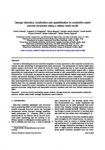
with CT). Besides, it is more expensive and less readily available than CT [132]. Therefore, CT is currently the preferred modality. MR plays a role in patients when radiation is undesirable, e.g., in pregnant patients or children. In the last few years, contrast-enhanced multi-slice x-ray computed tomography (CT) has become the preferred initial imaging test (and often the only test) to diagnose PE, for reasons that have already been mentioned before: it is a simple, minimally invasive, accurate and a very fast imaging technique [66, 128, 129, 136] that allows the direct depiction of a clot inside the blood vessels. Since its introduction of spiral CT in the early 1990s, it has gained wide acceptance as a first-line imaging test for PE [51, 123]. While the first single-slice scanners were limited in spatial resolution and scan time, and therefore less suited for depiction of subsegmental emboli, these limitations have been overcome by the advent of multi-slice scanners. The introduction of multi-slice CT has substantially improved the spatial resolution and scan times. A CT scan of the pulmonary arterial tree can be acquired up to the eighth branch in less than 10 seconds [51, 59]. The CT image can also be used to identify alternative potentially life-threatening causes of signs and symptoms in a patient with chest pain [137]. Diagnosis with Computed Tomography A CT scanner uses x-rays. The CT image consists of attenuation (absorbtion) differences of the various tissues, transferred into different grey levels: bones are white, tissue and blood are grey, and air is black. Contrast material (iodine) is injected into the vascular system with a relatively high flow and CT data is acquired during the ‘first pass’ of the contrast through the vessels, before the contrast material diffuses from the intra-vascular in the extra-vascular (organ) space. The CT scan of strongly contrast-enhanced blood vessels is called CT angiography (CTA). In CTA images the blood vessels appear as bright tubular structures (Figure 1.1) because the contrast material is dissolved in blood.

1 R

L

5 R

2 4

3 L

R

6

Figure 1.1: Three axial CT images from top to bottom showing (1) the aortic arch, (2) ascending aorta, (3) descending aorta, (4) main pulmonary artery, which is bifurcating in the left and right pulmonary artery, (5) superior vena cava and the (6) left atrium, which is connected to the pulmonary veins. An embolus causes an intravascular contrast defect, and therefore, is seen as a

14

Introduction

dark spot in the pulmonary arteries (Figure 1.2).

P E

Figure 1.2: PE appears as a filling defect inside the pulmonary arteries in CT images.

For a radiologist, it can be difficult to detect all PE in the CT data [143] for several reasons. The CT scanner produces consecutive 2D x-ray images of 512x512 pixels (picture elements), as a stack of approximately 400 cross-sectional slices so that a three-dimensional (3D) volume is constructed. In a 3D volume, the pixels are called voxels (volume pixels), of which the size is approximately 0.6 mm in every direction. The several hundred high-resolution images consisting of 100 million voxels have to be reviewed. Furthermore, the lung vasculature is quite complex with many segmental and subsegmental branches. It is almost impossible to visualize all vascular structures within one image at a time. Therefore, many radiologists go through such a scan several times reviewing only parts of the vascular system in the attempt not to miss an intravascular (sometimes very small) black dot indicating PE. A secure diagnosis or exclusion of PE is therefore quite time-consuming and highly dependent on the experience of the radiologist. For a radiologist, it might also be difficult to avoid false detections. There are several diagnostic pitfalls [63, 124, 165]:


15

Examples of diagnostic pitfalls are: • A poorly enhanced vein. Since PE are arrested in pulmonary arteries, the scan is optimized for enhancement of the arteries and the veins are often poorly filled with contrast material. These filling defects in the veins look similar to PE and might be misdiagnosed if the radiologist misinterprets the location. • Lymphoid tissue that is located around the vessels. Because it has the same intensity as PE, it might be misinterpreted as wall adherent thrombi. • Respiratory or cardiac motion, which may cause movement artifacts in the CT image with inhomogeneous intravascular contrast resembling PE. • Streak-artifacts near the superior vena cava due to beam hardening. • Parenchymal diseases alter the pulmonary perfusion and thus the difference between intravascular and extravascular contrast, hampering the diagnosis of PE. • Blurring due to the partial volume effect at the vessel wall or at bifurcations. • Impacted bronchi mimic dark tubular structures. • Incorrect bolus timing resulting in insufficient intravascular contrast. • Image noise due to low dose or obese patients. • Artifacts due to edge-enhancing image reconstruction. Because it is difficult and time consuming for a radiologist to find all emboli, a computer aided diagnosis (CAD) system is desirable. In current clinical practice, the diagnosis of PE is divided in a yes-or-no decision, independent of the location and severity of emboli (with some exclusions as stated before). It is therefore less important that CAD finds more emboli in a patient with already known disease. More important tasks of CAD seem to be: to increase the radiologists certainty to rule out a disease, to estimate the obstruction index [121] or to decrease inter-reader variability. In this thesis, we propose a CAD system for the automatic detection of PE in CTA images. For the design of such a system, the mentioned pitfalls must be taken into account, to avoid a large number of false detections. Therefore, our data were selected to demonstrate a variety of thrombus load and considerable differences in image quality with respect to motion artifacts, sub-optimal contrast enhancement and parenchymal diseases. This is important because the main problem of PE detection is the separation between true PE and look-alikes, which is much harder when the patient is suffering from overlying disease and image quality is suboptimal.

16

1.3

Introduction

Outline of the Thesis

Both stenosis and pulmonary embolism can obstruct the blood flow in vessels, which may have serious consequences. This thesis focusses on computer assistance for the diagnosis of these two types of obstructions. The first part discusses vessel quantification to improve the selection of patients with stenosis. The second part describes a CAD system for the automatic detection of PE which may be help a radiologist to find all emboli. The first part is about fast and accurate vessel-diameter quantification in CT images. Gaussian derivatives are commonly used as differential operators to localize the vessel wall. Chapter 2 describes how Gaussian derivatives should be computed on multi-dimensional data with anisotropic voxels and anisotropic blurring. In the CT images the voxels and blurring are usually anisotropic, which means that the voxel size and the amount of blur in the x- and y-directions are not equal to that in the z-direction. Although isotropic reconstruction is becoming more and more common for CT data, being able to handle anisotropic data (especially anisotropic blur) will continue to be important for image analysis, also in the medical field. In Chapter 3, we show that the computational cost of interpolation and differentiation on Gaussian blurred images can be reduced by using B-spline interpolation and approximation, without losing accuracy. Chapter 4 introduces a derivative-based edge detector with unbiased localization on curved surfaces in spite of the blur in CT images. In the last chapter of the first part, Chapter 5, we propose a modification of the full-width at half-maximum (FWHM) criterion to create an unbiased method for vessel-diameter quantification in CT images. This criterion is not only cheaper but also more robust to noise than the commonly used derivative-based edge detectors. The second part of this thesis describes the CAD system for automatic detection of PE in CTA images. The system consists of three steps, which are described in separate chapters. In the first step, pulmonary vessels are segmented and PE candidates are detected inside the vessel segmentation, as described in Chapter 6. Subsequently, shown in Chapter 7, features are computed on each of the candidates to enable the classification of the PE candidates. In the last step, classification is used to separate candidates that represent real emboli from the other candidates. The system is optimized with feature selection and classifier selection, and after that, the system for embolus detection is evaluated and results are presented in Chapter 8. Finally, the discussion can be found in Chapter 9, combined with some recommendations for future research.

Part I


17

Chapter 2

Gaussian Derivatives on Anisotropic Data Abstract – Gaussian derivatives are often used to analyze the structure in medical images. In this chapter, we show how Gaussian derivatives should be applied to multi-dimensional data with anisotropic blurring and anisotropic voxel sizes, with special attention to three-dimensional computed-tomography (CT) data.

19

20

Gaussian Derivatives on Anisotropic Data

2.1

Introduction

Computer vision tries to automate the interpretation of structures in an image. The low-level image structure is usually analyzed with differential operators. Gaussian derivatives are often used as differential operators. They are used to implement differential invariants – such as edge detectors, shape descriptors and motion estimators. In the medical field, Gaussian derivatives are commonly used to compute features for computer-assisted interpretation of multi-dimensional images. Interpolation and differentiation methods usually assume the images to be represented by a set of uniformly-spaced samples that are isotropically blurred. However, multi-dimensional images – e.g., from a computed-tomography (CT) scanner – usually are anisotropic in two ways (Figure 2.1). On one hand, the volume elements (voxels) are anisotropic if the voxel sizes are not equal in every direction. On the other hand, the blurring is anisotropic if the point-spread function (PSF) is not equal in every direction. Differential operators will only produce meaningful values if both types of anisotropy are taken into account. For example, isophote curvature – which shows in three-dimensional data the curvedness of a surface of equal intensity – will only be inversely proportional to the radius of the circles that locally fit to the shape of the isophotes if the blurring is isotropic. And the gradient magnitude will only reflect the slope of an edge if the voxel sizes are taken into account. Unfortunately, the anisotropy is often neglected, which leads to incorrect measurements. In this chapter, we will present a review on the computation of Gaussian derivatives on multi-dimensional images with anisotropic blurring and anisotropic voxels, with a special attention to three-dimensional CT images. The chapter is organized as follows. We will analyze the anisotropy due to blurring in Section 2.2, and the anisotropy due to voxel sizes in Section 2.3. In Section 2.4, an experiment is performed to verify the theory about Gaussian derivatives on anisotropic data.

C o n tin u o u s O b je c t

A c q u is itio n

B lu r r in g

S a m p lin g

D ig ita l Im a g e

Figure 2.1: The acquisition process of digital images can be modelled by acquisition, blurring and sampling. Blurring and sampling are often anisotropic.

2.2 Anisotropic Blurring

2.2

21

Anisotropic Blurring

In this section, we will first analyze how blurring is modelled in CT data. After that, we show how the anisotropy of blurring can be taken into account to extract meaningful features from the data.

2.2.1

Point-Spread Function (PSF)

In physics, an integrated weighting over the detector area is needed to perform a measurement. This causes a blurring effect. In CT images the blurring is a function of the beam collimation, detector size, interpolation algorithm, slice thickness, pitch, focus-center and focus-detector distances. The blurring due to all of this is modelled as a convolution by the PSF; a point in the object is not reproduced as a point, but as a spreaded point in the image. The PSF in CT images is often approximated by a Gaussian [113]. The PSF describes the impulse response of a system and its width is a measure of spatial resolution, which is often not the same in every direction. Therefore, the PSF is often approximated with an anisotropic Gaussian: 1 1 ~x ~x GN (~x, ~σ ) = exp − · (2.1) 2 ~σ ~σ (2π)N/2 det(~σ I) where N is the number of dimensions, ~σ is the vector that contains the standard deviations for each direction, and I represents the N × N identity matrix. The PSF can be obtained in two ways. One way is to measure the PSF directly as the edge-spread function (which leads to the integral of the PSF, as the Heaviside step function is the integral of the Dirac delta function), the line-spread function or (literally) as the point-spread function [113, 11, 92, 28]. Another way is to first measure its Fourier counterpart – the modulation transfer function (MTF) – and then transform the MTF to the PSF. Because the MTF is the most fundamental measurement of spatial resolution used in radiology [11], we will elaborate on its relation with the PSF, and how the MTF can be measured directly.

2.2.2

Modulation Transfer Function (MTF) and the PSF

The MTF is another way to describe the blurring in CT images. The MTF is the absolute value of the normalized complex Fourier transform of the PSF. In 2D: R ∞ R ∞ PSF(x, y) e−2 π i (u x + v y) dx dy −∞ −∞ R∞ R∞ (2.2) MTF(u, v)2D = PSF(x, y) dx dy −∞ −∞

In this equation u and v are spatial frequencies of the two-dimensional Fourier transform. The one-dimensional Fourier transform is defined as: s Z ∞ |b| F {h(x)} = h(x) ei b ω x dx (2.3) (2π)1−a −∞

22


where the parameters should be chosen as: a = 0 and b = −2π. Since the Fourier transform of a Gaussian is a Gaussian, and if the PSF can be modelled by a Gaussian, the relation between the PSF and the MTF can be written in two short equations: ⇒

MTF =

F −1

M T F = (2π)N/2 det(~σ I) GN (~ν , ~σ )

2.2.3

GN (~ν , 2π1 ~σ ) (2π)N/2 det(~σ I) 1 ) P SF = GN (~x, 2π ~σ

F

P SF = GN (~x, ~σ )

⇒

(2.4) (2.5)

Measuring the MTF

The MTF can be measured by using a test pattern that consists of a series of line pairs (i.e. bars and spaces, or square wave). It should be measured with a sine wave, but this is much more expensive to make. That is why everybody measures in practice with a square wave. In an acquired image, the response of a line pair consists of a part with a high value and a low value (Figure 2.2). The relative amplitude of this response is called contrast. As the spatial frequency of the line pairs per centimeter (lp/cm) increases – the pairs become smaller – the contrast decreases due to blurring. .50

.50

.25 .00

Test pattern Frequency ν

0.5

1.

1.5

2.

.25

.00

0.5

1.

1.5

2.

x HcmL

.00

-.25

-.25

-.25

-.50

-.50

-.50

0.5 lp/cm

1.0 lp/cm

.50

.50

.25

x HcmL 0.5

1.

1.5

1.5

2.

x HcmL

.25 0.17 x HcmL 0.5

1.

1.5

.00

2.

-.25

-.25

-.50

-.50

-.50

0.89

x HcmL 0.5

-.25

1.00

1.

2.0 lp/cm

.00

2.

0.5

.50

0.45

.25

.00

Response r(ν) Contrast

.50

.25 x HcmL

1.

1.5

2.

0.34

Figure 2.2: Response r(ν) of a bar pattern. The square-wave response is obtained with σpsf = 0.13cm. The frequency-contrast response of a square wave is shown as a solid curve in Figure 2.3). The three dots on this curve are obtained with the frequency and contrast quantities in Figure 2.2. However, the MTF is not equal to the frequency-contrast response of a square wave [140], but to the response of a sine wave. The sine-wave response R(ν) can be expressed in the square-wave response r(ν) as shown by Coltman [30]. The seventh-order approximation of this relation is: r(3ν) r(5ν) r(7ν) π r(ν) + − + ... (2.6) R(ν) = 4 3 5 7

2.2 Anisotropic Blurring

23

1 0.75 0.5 0.25 0.5

1.44

3

ν (lp/cm)

Figure 2.3: The frequency-contrast response of a sine wave (dashed curve) is equal to the MTF. The response of a square wave (solid curve) obtained from Figure 2.2 is not equal to the MTF.

With this equation, the square-wave response (solid curve in Figure 2.3) can be converted to the MTF (the dashed curve in Figure 2.3). The two ways to measure the amount of blur – in the frequency domain (MTF) and in the spatial domain (PSF) – can be compared. For example, the width of the PSF that was used to blur the bar pattern in Figure 2.2 (σ = 0.13 cm), can also be estimated in the frequency domain. A measurement of the width at halfmaximum (ν) of the MTF results in an estimate of ν = 1.44 lp/cm (see dashed curve in Figure 2.3). The computation of the PSF as a Fourier transform of the MTF results in the same estimate of σ: G1 (1.44, σ 12π ) √ = 0.5 (σ 2π)

⇒

σ = 0.13 cm

(2.7)

As shown, the blur can be measured with bar-shaped line pairs in the frequency domain and as the PSF in the spatial domain. Both methods result in the same estimate of blur and they can be transformed from one to the other and vice versa with a Fourier transform. The MTF or PSF should be measured in every direction to estimate the anisotropic blurring in multi-dimensional data.

2.2.4

Correction for Anisotropic Blurring

The blurring of the PSF in the z-direction is usually much larger than the blurring in x- and y-direction; the blurring is anisotropic. As mentioned before, the blurring must be made isotropic to produce a meaningful measurement. The total blur σtot in a processed image consists of two parts. The first is caused during acquisition by the PSF σpsf , and the second is caused by the Gaussianderivative operators σop . The self-similarity (or semi-group) property of the Gaus2 2 2 sian (σtot = σpsf + σop ) can be used to correct for the anisotropy of the PSF. The property of separability allows us to apply the operator in each of the directions

24


with a different value for σop in order to make the total blurring σtot equal in all directions. In some cases it is undesired to increase the amount of blur, because information is lost. However, in many cases extra blur is necessary to obtain accurate measurements. For example, an iso-surface on the boundary of a sphere with anisotropic blurring is not spherical anymore. Therefore, the isophote curvature will fail to represent the inverse of the radius. Additional blur can make the total blurring equal in all directions. So, we showed how the (anisotropic) blurring in data can be measured with the PSF and the MTF, and how the blurring can be made isotropic to allow analysis of the structure in images.

2.3

Anisotropic Voxels

In this section, the anisotropy of voxels is analyzed. We will first mention the terminology that is common for CT data. After that, we show how differential operators can take the anisotropy of voxels into account.

2.3.1

CT Terminology

The elements inside a CT volume are called voxels. However, the volumetric dataset can also be described as a ‘stack of slices’, and the elements inside a slice are called picture elements (pixels). In the x- and y-direction, the distance between the elements is called ‘pixel spacing’ and in the z-direction it is called ‘spacing between slices’ (according to the DICOM standard, the standard for medical imaging). The pixel spacing is equal to the division of the field-of-view size by the dimensions of a slice. The spacing between slices is equal to the reconstruction interval. The spacing between slices is easily confused with the slice thickness. Slice thickness is not the same as the size of the voxels, but it is related to the blurring of the data. In other words, the slices can be overlapping. For single-detector CT, slice thickness was directly related to slice collimation and pitch. For multi-detector CT the reconstruction algorithm allows the user in the same study to reconstruct images with high resolution but increased noise (thin slices) and images with lower resolution but less noise (thicker slices).

2.3.2

Natural Coordinates

Differential operators are not scale-invariant. This means that the slope of a blurred signal will decrease as the amount of blurring increases. Blur removes low-scale structure (like noise) and allows analysis at a higher scale. If we consider the transformation x → x/σ = x ˜, then x ˜ is dimensionless and the operator is scale-invariant. The dimensionless coordinate is called the natural coordinate [64]. This implies that the derivative operator in dimensionless natural coordinates has a scaling factor: ∂n n ∂n ∂xn → σ ∂ x ñ . The natural coordinates and the scaling factor avoid the decrease of the output of an image derivative at a larger scale.

2.3 Anisotropic Voxels

2.3.3

25

Correction for Anisotropic Voxels

In order to correct for the anisotropy of voxels we will perform a transformation to natural coordinates. Our goal is to make operators that are independent of the voxel size, which avoid the decrease of intensity for larger voxels. The length of a voxel in the x-direction will be defined as cx . Normalizing the Gaussian G1 (cx x, σ) requires a scaling factor cx : Z 1 cx x (2.8) cx G1 (cx x, σ) dx = erf( √ ) 2 2σ

where the units are pixels [px] for x and [mm/px] for cx . Applying the chain rule results in: ∂ nx {G1 (cx x, σ)} ∂ nx {G1 } cx = c1+nx (cx x, σ) (2.9) x nx ∂x ∂xnx where nx is the nxth-order derivative in the x-direction. So, in 3D, we can either transform the σ’s: σx σy σz ∂ nx ∂ ny ∂ nz {G3 (~x, [ , , ])} = nx ny nz ∂x ∂y ∂z cx cy cz nx ny nz ∂ ∂ ∂ σx σy σz c−nx c−ny c−nz {G3 }(~x, [ , , ]) (2.10) x y z ∂xnx ∂y ny ∂z nz cx cy cz or we can transform the coordinates x, y and z: ∂ nx ∂ ny ∂ nz {G3 ([cx x, cy y, cz z], ~σ )} = ∂xnx ∂y ny ∂z nz ∂ nx ∂ ny ∂ nz c1+nx c1+ny c1+nz {G3 }([cx x, cy y, cz z], ~σ ) x y z ∂xnx ∂y ny ∂z nz

(2.11)

Equation (2.10) or (2.11) makes the Gaussian derivatives invariant to the size of the voxels. If we assume isotropic pixel spacing (cx = cy ) and another value for the spacing between slices (cz ), then the anisotropy (a) is: cz cz a= = (2.12) cx cy If the coordinates are transformed so that pixel spacing in the x- and y-direction is defined to be the unit length, then only a scaling factor is required and we can use: ∂ nx ∂ ny ∂ nz n σz o [x, y, z], [σ , σ , G ] = x y 3 ∂xnx ∂y ny ∂z nz a σz ∂ nx ∂ ny ∂ nz 1 {G } [x, y, z], [σ , σ , ] (2.13) 3 x y anz ∂xnx ∂y ny ∂z nz a Equation (2.10) or (2.11) makes the Gaussian derivatives invariant to the size of voxels. These equations can easily be modified for n-dimensional data. In some cases in 3D data, invariance to anisotropy in the z-direction is sufficient; assuming that voxels are isotropic in the x- and y-direction. Equation (2.13) shows how the operators can be made invariant to this type of anisotropy.

26

2.4


Experiments and Results

To verify the theory about Gaussian derivatives on data with anisotropic blurring and anisotropic voxels we will perform an experiment with a synthetic image of a sphere. The sphere M is defined with a radius R, and a heaviside unit-step U: M = U(R − r). The blurred sphere is defined as: L = M ∗ G. Partial derivatives will be denoted by subscripts, as in Mz for ∂M ∂z . Derivatives are calculated in a locally fixed coordinate system (gauge coordinates). The vector w is defined in the direction of the gradient. Thus, Lww is the second-order Gaussian derivative in the gradient direction. The position vector, expressed in spherical coordinates is: ~r = [r cos(θ)sin(φ), r sin(θ)sin(φ), r cos(φ)]T . As the sphere is rotationally symmetric, we can solve it in 1D, along the radial direction only. We choose the derivatives to x and y to be zero (Lx = 0, Ly = 0) and the gradient magnitude as Lw = |Lz |, without loss of generality. Mz = − cos(φ)δ(R − r) R ∞R πR 2π ~) dΘdΦdρ Lz = 0 0 0 ρ2 sin(Φ)Mz G(~r − ρ r R cos(Φ) R r 2 +R2 R π sin(Φ) cos(Φ) e σ 2 dΦ (2.14) 0 √ = −e− 2 σ2 2

− r 2+R σ2

2

Lw = e

(r R+σ2 )e

−rR σ2

√

2 π σ3

rR

+(r R−σ 2 ) e σ2

2 π r2 σ

Lww can be derived from Lw , and the Laplacian (∆L) from these two. Lww =

(r+R)2 2σ 2

2rR 3 2 σ2 (r R + 2rRσ ) 1 + e + 2π 2rR (2σ 4 + r2 (R2 + σ 2 )) 1 − e σ2

−

e √

∆L = e−

r3

σ3

(r+R)2 2σ 2

rR

2rR 1+e σ2

2

2

+(R +σ ) √ 2π r σ 3

2rR 1−e σ2

(2.15)

The blurred sphere L can be derived from Lw by integration. L=

−σ e−

(r−R)2 2σ 2

+ σ e− √ 2π r

(r+R)2 2σ 2

1 − erf 2

r−R √ 2σ

1 + erf 2

r+R √ 2σ

(2.16)

Equation 2.16 is used to create a synthetic image of a blurred sphere (R = 4.4mm) without aliasing (σ = 1.5mm) on anisotropic voxels (cx = cy = 1.0mm/px, cz = 1.5mm/px, a = 1.5). Extra blurring (σ = 1.4mm) is applied in the z-direction to make the blurring√anisotropic. An extra blurring of σ = 1.4mm results in a total blurring of σz = 1.52 + 1.42 = 2.05 mm in the z-direction. Three cross sections through the center of the blurred sphere are shown in Figure 2.4. Note that in the figure the domain on the horizontal axis in the z-direction differs from the domains in the x- and y-direction. The lack of a flat plateau in the center of the sphere is caused by the amount of blurring in relation to the radius of the sphere.

2.5 Conclusions

27

I

I

I

1

1

1

0.8

0.8

0.8

0.6

0.6

0.6

0.4

0.4

0.4

0.2

0.2 -12 -9 -6 -3 0

3

6

9 12 15

x(px)

0.2 -12 -9 -6 -3 0

3

6

9 12 15

y(px)

-8 -6 -4 -2 0

2

4

6

8 10

z(px)

Figure 2.4: Creation of a blurred sphere (R = 4.4mm) with anisotropic voxels (cx = cy = 1mm/px, cz = 1.5mm/px) and anisotropic blurring (σxy = 1.4mm, σz = 2.05mm).

The image with anisotropic blurring and anisotropic voxels is used to show that we can calculate derivatives that match the theory. The second-order derivative in the gradient direction Lww is calculated on this image using Gaussian differential operators as in Eq. 2.13 with a total blurring of σtot = 3.4mm. The result is compared with Equation 2.15 (Figure 2.5). The root-mean-square (RMS) error appears to be 1.5 · 10−8 . Lww

Lww

Lww

0.01

0.01

0.01

0.005

0.005

0.005

-12 -9 -6 -3 0

3

6

9 12 15

x(px)

-12 -9 -6 -3 0

3

6

9 12 15

y(px)

-8 -6 -4 -2 0

-0.005

-0.005

-0.005

-0.01

-0.01

-0.01

-0.015

-0.015

-0.015

-0.02

-0.02

-0.02

2

4

6

8 10

z(px)

Figure 2.5: Lww calculated on a sphere (R = 4.4mm) with anisotropic voxels (cx = cy = 1mm/px, cz = 1.5mm/px) and anisotropic blurring (σxy = 1.4mm, σz = 2.05mm). The total blurring for Lww is σ = 3.4mm. The result of the differential operators (dots) matches Equation 2.15 (curve).

In this experiment we showed that the Gaussian derivatives can be used on data with anisotropic blurring and anisotropic voxels. The experimental results match the theory with an RMS value that is close to the computational accuracy.

2.5

Conclusions

In this chapter, a review was given on the computation of Gaussian derivatives on multi-dimensional images with anisotropic blurring and anisotropic voxels, with a special attention to three-dimensional CT images. The blurring in CT images is modelled by the PSF or the MTF. The blurring is usually anisotropic, which makes many differential operations (e.g., isophotecurvature computation) meaningless. Separability and the self-similarity (or semi-

28


group) property allowed a correction for anisotropic blurring. The voxel sizes in CT images are defined by the pixel spacing and the spacing between slices. The voxels are usually anisotropic, which should also be taken into account to create meaningful measurements. An approach, exploiting natural coordinates, allowed us to make the Gaussian derivatives invariant to voxel sizes.

Chapter 3

Gaussian Derivatives based on B-Splines H. Bouma, A. Vilanova, J. Oliv´ an Besc´ os, B.M. ter Haar Romeny and F.A. Gerritsen; Int. Conf. Scale Space and Variational Methods [15] c 2007 Springer-Verlag, http://www.springer.com/lncs Copyright

Abstract – Gaussian derivatives are often used as differential operators to analyze the structure in images. In this chapter, we will analyze the accuracy and computational cost of the most common implementations for differentiation and interpolation of Gaussianblurred multi-dimensional data. We show that – for the computation of multiple Gaussian derivatives – the method based on Bsplines obtains a higher accuracy than the truncated Gaussian at equal computational cost [15].

29

30

3.1

Gaussian Derivatives based on B-Splines

Introduction

Computer vision aims at the automatic interpretation of structures in an image. The low-level image structure is often analyzed with differential operators, which are used to calculate (partial) derivatives. In mathematical analysis, the derivative expresses (x) (x) = limh↓0 f (x+h)−f ). However, the slope of a continuous function at a point ( ∂f∂x h differentiation is an ill-posed operation, since the derivatives do not continuously depend on the input data [65]. The problem of an ill-posed differentiation on a discrete image F is solved through a replacement of the derivative by a (well-posed) convolution with the derivative of a regularizing test function φ [138, 52]. Z ∞ n F (ξ) ∂i1 ...in φ(x + ξ) dξ (∂i1 ...in F ∗ φ)(x) = (−1) −∞ Z ∞ F (ξ) ∂i1 ...in φ(x − ξ)dξ = (F ∗ ∂i1 ...in φ)(x) (3.1) = −∞

The Gaussian is positive (which avoids overshoot and ringing artifacts) and an integration over the kernel is normalized to one. These properties imply that variation will diminish, which means that the Gaussian is causal. The Gaussian is the only regularizing test function that is smooth, self-similar, causal, separable and rotation invariant [52, 43]. The convolution of an image with a Gaussian is called blurring, which allows the analysis at a higher scale where small structures (e.g., noise) are removed. Thanks to the mentioned properties, the Gaussian derivatives are often applied in the fields of image processing and computer vision as differential operators [64]. They are used to implement differential invariant operators – such as edge detectors, shape descriptors and motion estimators. In the medical field, the Gaussian derivatives are used to compute features in huge multi-dimensional images for a computer-aided interpretation of the data, sometimes even at multiple scales [107]. This processing requires an efficient and accurate implementation of the Gaussian derivatives. The naive approach to obtain the blurred derivatives of an image, is to convolve a multi-dimensional image with a multi-dimensional truncated Gaussian (derivative) kernel. The same result can be obtain with lower computational cost by using separability, because the rotation-invariant multivariate Gaussian is equal to a product of univariate Gaussians. However, the cost of both approaches increases as the scale gets larger. Therefore, many techniques are proposed for an efficient implementation at large scales or at multiple scales. The FFT [58] allows the replacement of an expensive convolution in the spatial domain by a cheaper multiplication in the Fourier domain. Usually, the cost of an FFT is only acceptable for large scales [53]. A recursive implementation [2, 36, 158] of the Gaussian (derivative) is even cheaper than the FFT [167], and the costs are – like the FFT – independent of the scale. However, this implementation lacks high accuracy, especially for small scales [10] and derivatives cannot be computed between voxels (e.g., for rendering) or locally at some voxels (e.g., to save time

3.1 Introduction

31

and memory for the computation of isophote curvature on a sparse surface). The low-pass pyramid technique [23, 33] uses down-sampling at coarser scales to reduce the computational cost. Especially analysis at multiple or higher scales can benefit from this approach. However, the use of large-scale Gaussian derivatives can be avoided because the Gaussian is a self-similar convolution operation. This means that a cascade application of two Gaussian kernels with p standard deviation σ1 and σ2 , results in a broader Gaussian function with σtot = σ12 + σ22 (semi-group property). Therefore, Lindeberg [97] proposed to first blur an image once with a large Gaussian G(σ1 ), and then obtain all partial derivatives at lower cost with smaller Gaussian derivative kernels g(σ2 ). In this chapter, we will compare the accuracy and computational cost of several approaches to obtain these derivatives. Figure 3.1 shows four ways to obtain a Gaussian derivative. One way is to convolve an image in one pass with a truncated Gaussian derivative for each partial derivative. The second way is the approach of Lindeberg [97] that first blurs an image once and then obtains all the partial derivatives with small truncated Gaussian derivative kernels. Due to truncation, the Gaussian is not continuous and smooth anymore, although the error of this exponential function rapidly approaches zero. In the third way, which is similar to the second way, the small Gaussian derivative is replaced by a B-spline derivative [23, 161, 160]. The higher-order B-spline β converges to a Gaussian as a consequence of the central-limit theorem. An advantage of the B-spline of order n is that it is a compact kernel that guarantees C n−1 continuity. The fourth way to compute the Gaussian derivatives makes a separation between blurring and differentiation. After blurring the image – an operation that can benefit from the mentioned optimizations – the derivative is computed without blurring. Many operators have been proposed to compute the derivative in an image (e.g., the Roberts, Prewitt and Sobel operators [1, 112, 146]). However, they do not compute the derivative without adding extra blur and they are very inaccurate. The unblurred derivative of an image can be computed as a convolution with the derivative of an interpolation function φ (4th way in Figure 3.1). The sincinterpolator is considered to be the perfect interpolator, because it can reconstruct band-limited signals from the sampled data without an error. However, in practice, the sinc-function cannot be used as interpolator because it requires an infinite kernel size and truncation leads to severe artifacts [105]. A quantitative comparison of several interpolation methods can be found in papers by Meijering et al. [109, 110], Jacobs et al. [73] and Lehmann et al. [91]. The comparisons show that for each of the methods for differentiation and interpolation there is a trade-off between accuracy, continuity and kernel size, and that B-spline interpolation [150, 152, 153] appears to be superior in many cases. Therefore, we used the derivative of a B-spline interpolator to implement the unblurred derivative (4th way in Figure 3.1). In the last decades, we have seen a growing competition between Gaussianand spline-based image-analysis techniques, which are both frequently used. To our knowledge, a comparison between the truncated Gaussian and the approaches

32

Gaussian Derivatives based on B-Splines g (s In p u t Im a g e

G (s 1)

G (s

to

to t

1 )

2 g (s 2) 3 b

B lu r r e d Im a g e (s 1)

B lu r r e d Im a g e (s t)

to t

)

4

B lu r r e d D e r iv a tiv e o f Im a g e

f

Figure 3.1: Four ways to obtain the blurred derivative of an image. The first way performs one convolution with the derivative of a Gaussian g(σtot ). The second and third way convolve the image with a Gaussian G(σ1 ) for most of the blurring and then with a smaller p derivative of a Gaussian g(σ2 ) or a B-spline derivative β; where σtot = σ12 + σ22 . The fourth way convolves the image with a Gaussian G(σtot ) for all the blurring and then with the derivative of an interpolator φ for differentiation.

based on B-spline approximation and B-spline interpolation (Figure 3.1) for a fast and accurate implementation of Gaussian derivatives has not been published before. In this chapter, we will compare the accuracy (Section 3.2) and computational cost (Section 3.3) of the four strategies.

3.2

Accuracy of Methods

In this section, the true Gaussian derivatives are compared to their approximations to analyze the accuracy of these approximations on one-dimensional data. Thanks to the separability of the Gaussian G, this analysis is also valid for higher dimensions. G(x, σ) =

x2 1 √ e− 2σ2 σ 2π

(3.2)

The error ǫ of an approximation y˜ of the true continuous signal y is computed as the normalized RMS-value, which is directly related to the energy. qR ∞ |˜ y (x) − y(x, σ)|2 dx −∞ qR (3.3) ǫ= ∞ 2 dx |y(x, σ)| −∞

For the normalized RMS-value, the error of the impulse response of a Gaussianderivative kernel that is truncated at x = aσ is independent of thepstandard deviation. For example, the normalized RMS-error is ǫ = 1 − erf(a), and p of a Gaussian 2 √ −a for a first-order Gaussian derivative: ǫ = 1 + 2 a e / π − erf(a).

3.2 Accuracy of Methods

3.2.1

33

Aliasing and Truncation of the Gaussian

Small-scale Gaussian operators may suffer from sampling artifacts. According to the Nyquist theorem, the sampling frequency must be at least twice the bandwidth in order to avoid overlap of the copied bands (aliasing) [64]. If the copies do not overlap, then perfect reconstruction is possible. For a small amount of blurring (e.g., σ < 1 pixel) limitation of the bandwidth of the reconstructed signal is not guaranteed and serious aliasing artifacts may be the result. Band-limitation is enforced by a convolution with a sinc function [10]. If high-frequencies are (almost) absent in the stop band, then aliasing is negligible and the signals with and without bandlimitation (g ∗φsinc (x) and g(x) respectively) are (approximately) equal. Figure 3.2a shows that sampling causes serious aliasing artifacts for a small-scale zeroth-order derivative of a Gaussian, and it shows that a first- or second- order derivative requires even more blurring for the same reduction of the aliasing effects. To avoid aliasing artifacts, second-order derivatives are often computed at σ = 2.0 pixels. Therefore, we will mainly focus further analysis on this amount of blurring (σtot = 2.0 px). For a fixed kernel size N , small scales will lead to aliasing artifacts but large scales will lead to truncation artifacts. The optimal trade-off between aliasing and truncation is selected by minimizing the difference between a band-limited Gaussian (g ∗ φsinc ) and a truncated p Gaussian. Figure 3.2b shows that the error is minimal at σ ≈ (N/6.25)0.50 ≈ N/6. If the truncated kernel is applied to a blurred input signal –pe.g. blurred by the PSF or pre-filtering with σ1 – so that the total blurring is σtot = σ12 + σ22 = 2.0 p px, the optimal scale can even be reduced to approximately σ2 ≈ (N/9.9)0.56 ≈ N/10, as shown in Figure 3.2c. The scale with a minimal error is used to implement the second approach in Figure 3.1. log(ǫ) 0.5

1

1.5 2

-2 1 -4

0

-6 -8

(a)

2

log(ǫ)

σ

4 -1 -2 -3 -4 -5 -6

5

6 7 4

8

log(ǫ)

N/σ 2 .0

9 10

-2

N/σ 1.8

7 8 9 10 11 12 13 14 4

8 -4

8

-6

12 16

12 16 -8

(b)

(c)

Figure 3.2: (a) The normalized RMS-error ǫ due to aliasing for a zeroth-, first- and second-order derivative of a Gaussian at σ = [0.5 − 2.0]. (b) The difference between a band-limited Gaussian and a truncated Gaussian is minimal at σ = (N/6.25)0.50 , where the kernel size N = [4, 8, 12, 16]. (c) On a blurred signal, the normalized RMS-error is minimal at σ = (N/9.9)0.56 .

34

3.2.2


B-Spline Approximation

The B-spline approximator is used to implement the third approach in Figure 3.1. A high-order B-spline [160], or a cascade application of kernels [161, 23], will converge to a Gaussian (central-limit theorem). The B-spline approximator β n (x) of order n is: n+1 n+1 1 X n+1 i n n (−1) µ x − i + (3.4) β (x) := i n! i=0 2 where µn (x) is xn for x ≥ 0 and zero for other values, and where n+1 is the i binomial coefficient. The derivatives of the B-spline can be obtained analytically in a recursive fashion based on the following property: ∂β n (x) 1 1 = β n−1 x + − β n−1 x − (3.5) ∂x 2 2 The z-transform [76] is commonly used in digital signal processing to represent filters in the complex frequency domain. For example, for cubic (n = 3) spline filtering, the z-transform is: B 3 (z) =

1 z −1 + 4 z 0 + 1 z 1 6

⇔

yi =

1 4 1 xi−1 + xi + xi+1 6 6 6

(3.6)

The output yi of this digital filter only depends on the inputs x, which makes it a finite impulse response (FIR) filter. The derivative of a B-spline approximator β n (x) can be used as a small-scale Gaussian derivative. Figure 3.3a shows the normalized RMS-error pbetween a Gaussian and a B-spline is minimal for the standard deviation σ = N/12 [151]. Although the B-spline converges to a Gaussian for higher orders, the error is not reduced for higher orders (Figure 3.3b) when it is applied to a blurred signal (to obtain σtot = 2.0 px). The scale with a minimal error is used to analyze the accuracy of this approach.

3.2.3

B-Spline Interpolation

The B-spline interpolator is used to implement the fourth approach in Figure 3.1. In order to perform B-spline interpolation of the blurred image H with the approxn imating B-spline kernels (β n in Eq. 3.4), an inverse operation Binv is required. ˜ = H ∗ Bn ∗ βn h inv

(3.7)

The inverse operator can easily be calculated in the z-domain as B n (z)−1 . To obtain a stable filter, this inverse operator can be decomposed by its negative roots with magnitude smaller than one [152, 153]. For example, √ the root of the inverse of a cubic B-spline (Equations 3.6 and 3.8) is λ = −2 + 3. −1

B 3 (z)

=

1 1 6 1 = 1 = −6λ B 3 (z) z + 4 + z −1 (1 − λz −1 ) (1 − λz 1 )

(3.8)

3.2 Accuracy of Methods

log(ǫ)

9 10 11 12 13 14 15 -0.5 -1 -1.5 -2

35

N/σ 2

4 16

log(ǫ)

-0.5 9 -1 -1.5 -2 -2.5 -3 -3.5

(a)

10 11 12 13 14

N/σ 2

16 4

(b)

Figure 3.3: The normalized RMS-error between a Gaussian and a B-spline p approximator is minimal at σ = N/12, for kernel size N = 4, 8, 12, 16. (b) The same relation can be found on a blurred signal. Multiplication of two parts in the z-domain is equivalent to a cascade convolution with both parts in the spatial domain. The last part in Equation (3.8), with z 1 , can be applied backward, so that it also becomes a z −1 operation. This results in a stable and fast filter, which should be applied forward and backward: 1 1 − λz −1

⇔

yi = xi + λ yi−1

(3.9)

The output yi of this digital filter does not only depend on the input xi , but also on the output yi−1 , which makes it a recursive – or infinite impulse response (IIR) – filter. The recursive inverse operation makes the B-spline interpolator computationally more expensive than the B-spline approximator at equal order n. For more information about B-Spline interpolation, we refer to the work of Unser et al. [152, 153, 150].

3.2.4

Comparison of Accuracy

An experiment was performed to estimate the normalized RMS-error between the impulse response of a continuous Gaussian derivative (σtot = 2.0 px to avoid aliasing) and each of the four approaches (Figure 3.1). Measuring for each approach the error of the impulse response gives an indication of the accuracy in general, because a discrete image can be modelled as a sum of impulses with varying amplitude. The first approach, which is based on a one-pass truncated Gaussian of σ = 2.0 pixels, used an unblurred impulse as input signal. The second and third approach, which are based on a small-scale truncated Gaussian and on a B-spline approximator, used a sampled Gaussian as an input signal to obtain a total blurring of σ = 2.0 pixels. The fourth approach, which is based on B-spline interpolation, used a sampled Gaussian of σ = 2.0 pixels as input signal. Truncation of the one-pass Gaussian is often performed at 3σ or 4σ, which corresponds to a kernel size of 12 or 16 pixels for σ = 2.0 pixels. Figure 3.4 shows

36


that for these kernel sizes the normalized RMS-error in the second-order derivative is 5.0 · 10−2 or 2.4 · 10−3 respectively. The results show that B-spline approximation requires much smaller kernels to obtain the same accuracy as the truncated Gaussian (4 or 6 px respectively). The figure also shows that B-spline interpolation and cascade application of small-scale Gaussians may be interesting if higher accuracies are required, but for most applications the approach based on B-spline approximation will be sufficiently accurate. log(ǫ) 4

6

8

10

-1

12

1:g(σtot )

-2

16

log(ǫ)

N

4

3:β

-4

2:g(σ2 )

-5

8

10

12

16

log(ǫ)

N

1:g(σtot )

4

6

8

10

12

14

16

N

1:g(σtot )

-1

3:β

-2

3:β

-3

-4

2:g(σ2 ) 4:φ

2:g(σ2 )

-4 -5

-6

0th order

14

-3

-5

4:φ

6

-1 -2

-3

-6

14

4:φ

-6

1st order

2nd order

Figure 3.4: The normalized RMS-error ǫ in estimating the zeroth-, firstand second-order Gaussian derivative (σ = 2.0px) for the four approaches based on the one-pass truncated Gaussian (g(σtot ), dashed), the cascade application Gaussians (g(σ2 ), dashed), the B-spline approximator (β, solid) and the B-spline interpolator (φ, solid). The first approach requires much larger kernels than the others to obtain the same accuracy.

3.3

Computational Cost

Our comparison of computational cost will focus on the calculation of first- and second-order derivatives at a low scale (σ = 2.0 px) in three-dimensional (3D) data, because these derivatives are frequently used in the medical field. For these parameters, we will show that – in most cases – it is beneficial to use the B-spline approximator. For larger scales, more derivatives or higher-dimensionality it will be even more beneficial to make a separation between the blurring and differentiation. Therefore, our analysis can easily be extended to the computation of an arbitrary number of derivatives at higher scales on multi-dimensional data. Figure 3.4 showed that the truncated Gaussian requires 12 or 16 pixels to obtain the same accuracy as the B-spline approximator of 4 or 6 pixels respectively. For these sizes thep B-spline approximator (B-spl.A) is more accurate than the cascaded Gaussians (G( N/10)) and computationally cheaper than the B-spline interpolator (B-spl.I ) because no inverse is required (Eq. 3.7). Therefore, we will focus on the

3.3 Computational Cost

37

comparison of the B-spline approximator with the truncated Gaussian. Despite its small kernel, the B-spline is not always cheaper than the truncated Gaussian because it requires preprocessing to obtain the same amount of blur. The computational cost of this global blurring step can be reduced – especially for large scales – by using a recursive implementation [158]. The estimation of the computational cost C is based on the number of multiplications, which is equal to the kernel size. Three approaches are distinguished to analyze the performance for different purposes (Table 3.1). In the first approach, all volume-elements (voxels) are processed in a 3D volume. In the second, the derivatives are computed at some voxel-locations, and in the third, interpolation and differentiation is allowed at arbitrary (sub-voxel) locations in the volume. Finally, our estimation of the computational cost is verified with an experiment. Table 3.1: The computational cost C in a 3D volume of d derivatives based on the truncated Gaussian (kernel size k) and B-spline approximation (order n).

Trunc. Gauss B-spline approx.

3.3.1

Blur – 3 (k + 1)

All Voxels 3 d (k + 1) 3 d (n)

Some Voxels d (k + 1)3 d (n)3

Some Points d (k)3 d (n + 1)3

Cost of Differentiation on All Voxels

The computation of Gaussian derivatives on all voxels allows the use of a separable implementation with discrete one-dimensional filters. The continuous B-spline of order n with kernel size n + 1 is zero at the positions −(n + 1)/2 and (n + 1)/2. Therefore, the number of non-zero elements in a discrete B-spline kernel is n. The truncated Gaussian with kernel size k is not zero at its end points and therefore it requires k + 1 elements in the discrete kernel to avoid the loss of accuracy. For a ‘fast’ computation (n = 3, k = 12) of three first-order derivatives on all voxels, the B-spline approximator is 1.8 times faster than the truncated Gaussian despite the required preprocessing. For the nine first- and second-order derivatives, the B-spline is 2.9 times faster. For a ‘more-accurate’ computation (n = 5, k = 16) of three or nine derivatives, the B-spline approximator is 1.6 resp. 2.5 times faster than the truncated Gaussian (horizontal lines in Figure 3.5).

3.3.2

Cost of Differentiation on Some Voxels

If only a small percentage p of the volume needs to be processed (e.g, to compute shape descriptors on the surface of an object) – or if storage of multiple derivatives of the whole image consumes too much memory – the non-separable implementation may be more efficient to compute the derivatives than the separable implementation. However, in 3D data, the cost of a non-separable local operation increases with a power of three instead of a factor of three (Table 3.1).

38


The non-separable implementation is more efficient than the separable for the ‘fast’ B-spline approximator (n = 3) if less than p = 33% of the volume is processed, and for the ‘more-accurate’ (n = 5) if less than p = 12% is processed (Figure 3.5). Figure 3.5 also shows that the B-spline implementation (n = 3, d = 3) is more efficient than the truncated Gaussian if more than p = 0.6% of the voxels is processed (d = 9 reduces the trade-off point to p = 0.2%). For example, the B-spline (n = 3, d = 9) is 8 times faster than the truncated Gaussian at p = 2.0%. If we would have assumed that the blurring for the B-splines was incorporated in the preprocessing, then the B-spline approximator would even have been 81 times faster than the truncated Gaussian for each voxel. Fast (n = 3, k = 12) 1000

0.1

C

1000

More accurate (n = 5, k = 16)

C

1000

C

1000

300

300

300

300

100

100

100

100

30

30

30

1

10

d=3

p

100

0.1

1

10

d=9

p

100

0.1

C

30 1

10

d=3

p

100

0.1

1

10

p

100

d=9

Figure 3.5: The curves show the computational cost C for processing a percentage p of the voxels with a non-separable implementation in a 3D volume with a truncated Gaussian (dashed) and the B-spline (solid) for d derivatives. The horizontal lines show the cost of processing all voxels with a separable implementation. The plots show that the B-spline is expected to be more efficient if more than p = 0.6% of the data is processed.

3.3.3

Cost of Interpolation and Differentiation on Arbitrary Points

To interpolate and differentiate at arbitrary (sub-voxel) points in the volume continuous kernels are needed and a separable implementation cannot be used. The n-th order B-spline has a continuous kernel size of n + 1 (Table 3.1). Figure 3.6 shows that if more than p = 0.8% of the data is processed the B-spline is more efficient than the truncated Gaussian. For example, if nine derivatives are computed at a number of points that equals p = 10% of the voxels, the B-spline (n=3) is more than 16 times faster than the truncated Gaussian (k = 12).

3.3.4

Validation of Cost of Differentiation on Voxels

To validate our estimation of the computational cost, we measured the time that was required to compute the nine first- and second-order derivatives on a 3D volume of 512x512x498 voxels with a Pentium Xeon 3.2 GHz processor. In this experiment, we compared the implementations based on the truncated Gaussian (k = 12) and

3.3 Computational Cost

39

Fast (n = 3, k = 12) 1000

0.1

C

1000

More accurate (n = 5, k = 16)

C

1000

C

1000

300

300

300

300

100

100

100

100

30

30

30

1

10

d=3

p

100

0.1

1

10

p

100

0.1

d=9

C

30 1

10

d=3

p

100

0.1

1

10

p

100

d=9

Figure 3.6: The computational cost C for processing arbitrary points as a percentage p of the voxels in a 3D volume with a truncated Gaussian (dashed) and the B-spline (solid) for d derivatives. The plots show that the B-spline is expected to be more efficient if more than p = 0.8% of the data is processed.

the B-spline approximator (n = 3) as an example to show that our assumptions are valid. The measured results in Figure 3.7 are in good agreement with our analysis. The measurements show that the B-spline is more efficient if more than 0.3% of the data is processed (estimated 0.2%). The B-spline appears to be 6 times faster than the truncated Gaussian if 2% of the volume is processed with a non-separable implementation (estimated 8 times faster). And if all voxels are processed with a separable implementation the B-spline appears to be 2.1 times faster (estimated 2.9 times faster). t (sec) 1000

300

100

30

0.1

1

10

p (%)

100

Figure 3.7: The measured computation time t in seconds for processing a percentage p of the voxels in a 3D volume (512x512x498 voxels) with a truncated Gaussian (k = 12, dashed) and a B-spline approximator (n = 3, solid) for 9 derivatives. The horizontal lines show the cost of processing all voxels with a separable implementation. The plot shows that, for equivalent accuracy, the B-spline is more efficient if more than p = 0.3% of the data is processed.

40

3.4


Conclusions

We analyzed the accuracy and computational cost of several common implementations for differentiation and interpolation of Gaussian blurred multi-dimensional data. An efficient implementation is extremely important for all fields that use Gaussian derivatives to analyze the structure in data. A comparison between an implementation based on the truncated Gaussian and alternative approaches based on B-spline approximation and B-spline interpolation has not been published before, to the best of our knowledge. If the vesselness or isophote curvature of a data set needs to be computed (requiring six or nine derivatives respectively), the B-spline approach will perform much faster than the approach based on truncated Gaussians. These operators are very important in the field of medical imaging for shape analysis. Our analysis shows that, for the computation of first- and second-order Gaussian derivatives on threedimensional data, the B-spline approximator is faster than the truncated Gaussian at equal accuracy, provided that more than 1% of the data is processed. For example, if 2% of a 3D volume is processed, B-spline approximation is more than 5 times faster than the truncated Gaussian at equal accuracy. Our analysis can be extended easily to an arbitrary number of derivatives on multi-dimensional data. Higher accuracy will not always lead to better results. However, in many cases, the same accuracy can be obtained at lower computational cost, as was shown in this chapter. Another advantage of the B-spline of order n is that C n−1 continuity is guaranteed, whereas the truncated Gaussian is not even C 0 continuous.

Chapter 4

Correction for the Dislocation of Curved Edges H. Bouma, A. Vilanova, L.J. van Vliet and F.A. Gerritsen, IEEE Trans. Pattern Analysis and Machine Intelligence [16] c 2005 IEEE, http://www.ieee.org Copyright

Abstract – Conventional edge-detection methods suffer from the dislocation of curved surfaces due to the PSF. We propose a new method that uses the isophote curvature to circumvent this. It is accurate for objects with locally constant curvature, even for small objects (like blood vessels) and in the presence of noise.

41

42

4.1

Correction for the Dislocation of Curved Edges

Introduction

Many clinical applications of medical imaging require that edges are accurately located. An example is the diagnosis of a vascular disease, where the grading of stenoses is an important factor in determining the treatment therapy [56]. However, inherent to the acquisition step is a blurring effect, which can be modelled by the convolution with a point-spread function (PSF). This blurring function causes conventional edge-detection methods to inaccurately locate edges, leading to errors in quantification and visualization. The dislocation of curved edges due to the PSF was shown several times in the literature. Vessel quantification measurements have shown that an adaptive threshold causes an error in the diameter estimation of cylindrical structures [56, 125, 71]. Frangi et al. [56] and Krissian et al. [89] used a simplified model to approximate the cross-section of a tube. Later, Krissian et al. [90] showed that the radius estimation of tubes in CT images can be improved by modelling the PSF correctly. Many deconvolution methods have been proposed to undo the blurring caused by the PSF, which include approximations of the inverse filter and iterative methods [79]. Most deconvolution methods are ill-posed and hence unstable and noise enhancing, which deteriorates the result [98]. Regularization can be used to reduce the sensitivity to noise, at the expense of a considerable increase in computational cost for iterative methods [25]. We propose a new non-iterative edge-localization method that yields an exact correspondence between the edge that is detected and the true surface of objects in the real word. The locally measured isophote curvature is used to correct for the dislocation of the curved surface due to Gaussian blurring, in 2D and 3D [14]. The analysis in this chapter and the proposed method are applicable where the images show rather homogeneous objects and where the PSF can be approximated by a Gaussian. Although the PSF is not completely isotropic and shift invariant for computed tomography (CT) [41], this approximation can safely be made for CT and several other medical acquisition modalities [113]. This chapter is organized as follows. In Section 4.2, existing methods for edge detection are summarized. In Section 4.3, the dislocation of curved edges is analyzed mathematically. An approximation for curved surfaces in 3D is made in Section 4.4. Section 4.5 is about the implementation of the proposed method. Finally, in Section 4.6, experimental results are discussed.

4.2

Existing Edge-Detection Methods

Object boundaries are usually detected with first- and second-order derivatives. The gradient, i.e. a vector of first-order derivatives, may indicate the presence of an edge and the maximum of the gradient magnitude is commonly used to locate edges. The zero-crossings of the second-order derivative in the gradient direction (Lww ) are located where the gradient magnitude is maximal [24]. For simplicity,

4.3 Analysis of Curved Edges and Surfaces

43

the zero crossings of the Laplacian (∆L), which is the trace of the Hessian matrix, can also be used to locate edges [104]. The Laplacian is easy to calculate, but the zero crossings are not located where the gradient is maximal [115, 157]. However, our goal is not to find the position of maximal gradient in the blurred image, but to find the location of the edge before blurring. For example, if the edge of a circular object with radius R is not defined as the position where the gradient is maximal after blurring, but as the location before blurring, the zero-crossing positions r0 of both methods (∆L and Lww ) give a dislocation of the curved edges. The dislocation (r0 − R) of these methods goes in opposite directions (Figure 4.1). ∆L gives an overestimation and Lww gives an underestimation of the radius. The dislocation is caused by the isophote curvature κ in relation with the standard deviation σ of the Gaussian blurring. Since both ∆L and Lww appear to be dislocated in opposite directions, Van Vliet and Verbeek [154] proposed the PLUS operator, which sums ∆L with Lww . This operator reduces the dislocation of curved edges. Mendon¸ca [111] recently proposed a two-step method that fits a curve through the zero crossings of Lww and corrects for the bias in the localization by shifting the curve according to the dislocation that is known if the curvature is locally constant. We will derive a filtering method that corrects for the dislocation and does not require curve extraction. The methods are analyzed in the next section. (r0 −R)/R 0.02 ∆L P LU S

0.00 0.1

σκ 0.2

Lww

-0.02

Figure 4.1: The zero-crossings r0 of the Laplacian (∆L) and the secondorder derivative in the gradient direction (Lww ) are dislocated in the opposite direction. Therefore, the PLUS operator (∆L + Lww ) was proposed by Van Vliet and Verbeek [154].

4.3

Analysis of Curved Edges and Surfaces

In this section, the dislocation of edge detectors is mathematically analyzed and a new operator is derived. The zero crossings of this operator are located exactly at surfaces with locally constant curvature. First, the notation, assumptions and problem definition are mentioned. The filter is derived for 2D and 3D in the Subsections 4.3.4 and 4.3.5 respectively. Finally, at the end of this section, conclusions will be drawn.

44

4.3.1


Background and Notation 2

∂ L Partial derivatives will be denoted by subscripts, as in Mx for ∂M ∂x or Lyy for ∂y 2 . Derivatives are calculated in a locally fixed coordinate system (gauge coordinates). The vector w is defined in the direction of the gradient and vector v (and u, in 3D) are perpendicular to w. Thus, Lww is the second-order derivative in the gradient direction. The first order derivative in the gradient direction (Lw ) is equal to the gradient magnitude and the first-order derivative tangential to the iso-surface (Lv ) is equal to zero. The isophote curvature in 2D is denoted by κ. In 3D, it consists of two values (the principal curvatures: κ1 and κ2 , sorted by magnitude: |κ1 | > |κ2 |). The vectors corresponding to these values are perpendicular to the gradient and perpendicular to each other. The sum of principal curvatures will be denoted as κΣ (= κ1 + κ2 ).

4.3.2

Assumptions

Three assumptions are made during the derivation. First, regions are assumed to be rather homogeneous. Therefore, edges can be modelled by the Heaviside unit step U(x). Second, the curvature is assumed to be locally constant. Locally constant curvature means that the curvature is constant inside the footprint of the blurring function. The unblurred objects M = U(R − r) with constant curvature will be a disk (interior of circle) in 2D, a ball (solid sphere) and a cylinder in 3D with radial coordinate r (distance to the origin) and radius R. Third, the shape of the PSF, which causes the blurring, is assumed to be Gaussian: ~r.~r 1 exp − 2 G= √ (4.1) 2σ ( 2πσ 2 )N where σ is the standard deviation, N is the number of dimensions and (~r.~r) is the dot product of the position vector with itself. In cartesian coordinates the position vector ~r = [x, y, z]T . The blurred object L is defined as an N-dimensional convolution: L = M ∗ G.

4.3.3

Problem Definition

The most commonly used edge detectors are the detectors of Canny [24] and MarrHildreth [104] based on Lww and ∆L, respectively. Figure 4.1 shows that both dislocate the edges in opposite directions. The PLUS operator (Lww + ∆L) results in an edge detector with a better localization. However, if σκ is larger than 0.2, the performance of the PLUS operator also diminishes (as shown in Section 4.6). The equation of the PLUS operator in 2D can be written as: 1 (4.2) PLUS = Lww + ∆L = 2 Lww − κ Lw 2


45

We want to correct for the dislocation of curved surfaces. Therefore, we use the curvature term in (4.2) to obtain a better localization. This can be achieved by solving: Lww − α(σ κ) κ Lw = 0

(4.3)

for the function α(σ κ), where α(σ κ) is expected to be approximately 0.5 for small values of σ κ (like the PLUS operator). The product of the standard deviation of the Gaussian blurring σ and the local isophote curvature κ is taken as the parameter of this function α(σ κ), because it is a dimensionless quantity and therefore scale invariant.

4.3.4

Curved Edges in 2D

The simplest object with (locally) constant curvature in 2D, is a disk M = U(R−r). The position vector, expressed in polar coordinates, is: ~r = [r cos(φ), r sin(φ)]T . The derivatives of M are: Mx = −cos(φ)δ(R − r) My = −sin(φ)δ(R − r) q Mw = Mx2 + My2 = δ(R − r)

Mww = ∆M =

Mx2 Mxx +2Mx Mxy My +My2 Myy = δ ′ (R Mx2 +My2 Mxx + Myy = δ ′ (R − r) − δ(R−r) r

(4.4) − r)

The gradient magnitude of the blurred object Lw can be obtained by the convolution of Mw with a Gaussian G. The final equations are rotation invariant. Therefore, we may choose Ly = 0 and Lw = |Lx | without loss of generality. Lx = Mx ∗ G R ∞ R 2π = 0 0 ρMx (~ ρ)G(~r − ρ ~)dΦ dρ R ∞ R 2π = 0 0 −ρ cos(Φ) δ(R − ρ) ρ2 +r 2 −2r ρ cos(φ−Φ) − 1 2σ 2 dΦ dρ 2πσ 2 e

(4.5)

2 2 − R2σ+r 2

1 = −R 2πσ 2 e R 2π r R cos(φ−Φ) σ2 dΦ cos(Φ)e 0

Lw =

R σ2

e−

R2 +r 2 2σ 2

I1 ( rR σ2 )

where In (·) is the modified Bessel function of the first kind. Lww can be derived from Lw . These results are in agreement with the result of Mendon¸ca [111]. As shown in (4.4), ∆L can be calculated from Lw and Lww . r 2 +R2 2 rR Lww = e− 2σ2 − R σ 4 I0 σ 2 + R rR (4.6) ( rσR 4 + rσ 2 ) I1 σ2 2 2 rR +R 2 − r 2σ R rR rR 2 − σ4 I0 σ2 + σ4 I1 σ2 ∆L = e

46


The curvature κ can be obtained from ∆L = Lww + Lvv = Lww − κ Lw . Notice that κ = 1/r. Finally, an edge detector with zero crossings at position r0 = R can be defined: Lww − α κ Lw = 0; and this equation can be solved for α. α = 1+

r2 σ2

−

= 1+

R2 σ2

−

rR r R I0 ( σ2 ) 2 σ I1 ( rR σ22 ) R 2 I0 2 R σ 2 σ I R2 1 σ2

(4.7) (at r = R)

Curvature is inversely proportional to the radius. This can be used to define α as a function of σ κ:   1 2 2 I 0 1 1 − σκ  α(σ κ) = 1 + (4.8) 1 2 σκ I 1

σκ

This equation is shown in Figure 4.2. If σκ approaches zero, then α = 0.5, and our operator becomes the PLUS operator. For σ κ > 0.5, the entire object is inside the center part of the Gaussian PSF. The α in (4.8) avoids dislocation of the zero crossings for an object with locally constant curvature in 2D. So, the proposed method can locate the edge of a disk without a bias. α 1.0

0.5 0.0 1

2

3

4

σκ

-0.5 -1.0

Figure 4.2: Function α in (4.8) allows the localization of edges with locally constant curvature in 2D without a bias.

4.3.5

Curved Surfaces in 3D

The curvature term of the PLUS operator in 3D depends on the sum of curvatures. PLUS = 2 Lww − 12 (κ1 + κ2 )Lw (4.9)

Therefore, the κ in the 2D problem definition is replaced by the sum of curvatures κΣ in 3D: Lww − α κΣ Lw = 0

(r = R)

(4.10)

Simple objects in 3D with constant curvature and different ratios of κ2 /κ1 are balls (κ2 /κ1 = 1) and cylinders (κ2 /κ1 = 0). Both objects are described below.


47

Ball The derivation for a ball is similar to that of a disk. The position vector, expressed in spherical coordinates is: [r cos(θ)sin(φ), r sin(θ)sin(φ), r cos(φ)]T . The derivatives of M are: Mx = −cos(θ)sin(φ)δ(R − r) My = −sin(θ)sin(φ)δ(R − r) Mz = −cos(φ)δ(R − r) q Mx2 + My2 + Mz2 = δ(R − r)

Mw =

Mww = (Mx2 Mxx + My2 Myy + Mz2 Mzz + 2(Mx (Mxy My +Mxz Mz )+My Myz Mz ))/ (Mx2 + My2 + Mz2 ) = δ ′ (R − r) ∆M = Mxx +Myy +Mzz = δ ′ (R − r) − δ(R−r) r

(4.11)

The gradient magnitude of the blurred object Lw can be calculated by a convolution. We choose Lx = 0, Ly = 0 and Lw = |Lz | without loss of generality. R ∞R πR 2π Lz = 0 0 0 ρ2 sin(Φ)Mz G(~r − ρ ~) dΘdΦdρ = −e−

r 2 +R2 2 σ2

2 2 − r 2+R σ2

Lw = e

Rπ

R

0

r R cos(Φ)

sin(Φ) cos(Φ) e σ2 √ 2 π σ3

(r R+σ2 )e

−rR σ2

√

dΦ

(4.12)

rR

+(r R−σ 2 ) e σ2

2 π r2 σ

Lww can be derived from Lw , and ∆L from these two. (r+R)2 − 2rR 2 3 2 σ2 + (r R + 2rRσ ) 1 + e Lww = e√2π 2σ r3 σ3 2rR (2σ 4 + r2 (R2 + σ 2 )) 1 − e σ2 ∆L = e−

rR

(r+R)2 2σ 2

2rR 1+e σ2

2

2

+(R +σ ) √ 2π r σ 3

2rR 1−e σ2

(4.13)

The sum of curvatures κΣ can be obtained with ∆L = Lww − κΣ Lw . Notice that the sum of curvatures on a ball is κΣ = 2/r, because each of the two principal components of isophote curvature is 1/r. Finally, an edge detector with zero crossings at position r = R can be defined: Lww − α κΣ Lw = 0; and this equation can be solved for α, resulting in: 4

2( R σ ) +2 1−e

α= 2 1−e

2

2

( Rσ )

( Rσ )

2

!

2

2

+( R σ) 2

+( R σ)

1+e

3+e

2

2

2

( Rσ )

2

( Rσ )

!

(4.14)

!!

Replacing R by 2/κΣ will define α to be a function of the product of κΣ and σ. α(σ κΣ ) =  2

2 σ κΣ

4



+2 1−e

2 1−e

2

2

2 σ κΣ

2 σ κΣ

2

+

2 

+

2 σ κΣ

2

2 σ κΣ



2

 1+e

2



 3+e

2 σ κΣ

2

2 σ κΣ

2  



2 



(4.15)

48


This equation is shown in Figure 4.3. It can be used to locate the edge of a ball without a bias. α 1.0

0.5 0.0 1

2

3

4

σκΣ

-0.5 -1.0

Figure 4.3: Function α in (4.15) can be used to locate the edge of a ball in 3D without a bias.

Cylinder For a cylinder, the 3D Gaussian can be decomposed in one component in the direction of the central axis of a cylinder (z-direction) and two components in the cross-sectional plane. Because all derivatives in the z-direction are zero, the solution for the cylinder is identical to that of the disk after replacing the 2D κ by the 3D κΣ in (4.8). This function α is used to accurately quantify the diameter of tubular structures (such as blood vessels).

4.3.6

Conclusion of the Analysis

A method for unbiased edge localization was derived for blurred disks, balls and cylinders. For small values of σ κ, function α approaches 0.5 and our operator approximates the PLUS operator, as expected. Increasing σ κ yields different values for α. Instead of extracting a contour in 2D at the zero crossings of Lww and estimating the required dislocation, as Mendon¸ca et al. proposed [111], we designed an edge-detector with its zero-crossings at the correct location that can also be applied in 3D. The analysis helps us to obtain a better understanding of the small-vessel radiusestimation results of others [56, 125, 71, 89], and it yields more accurate quantification. The accuracy of the new edge detector will be verified in Section 4.6. The function α(σ κΣ ), which avoids dislocation, is not invariant to the ratio between the principal isophote curvatures. α is not the same for a cylinder (κ2 /κ1 = 0) and a ball (κ2 /κ1 = 1). It is different for small values of σκ (e.g., for σκ smaller than 0.2). Therefore, a more general approximation for curved surfaces is presented in the next section.

4.4 Approximation for Curved Surfaces in 3D

4.4

49

Approximation for Curved Surfaces in 3D

Because α is not invariant to the ratio κ2 /κ1 , the sum of curvature components does not give enough information to correct for the dislocation of the curved surface. Therefore, not only the sum of curvature components, but also the ratio between the curvature components is used to correct for the dislocation. These two dimensionless parameters allow the creation of a two-dimensional look-up table in a limited domain, with σ κΣ (that was used in the previous section) on one of the axis. An approximation of α as a function of σκΣ and κ2 /κ1 is: α(σ κΣ , κκ12 ) ≈ −1 + e

κ22 2 κ21

(σ κΣ )2 4

+

3 2

−

κ22 2 κ21

6.7−7.2 · 1.0374

2

( 25 − 4κκ12 )

!

(4.16)

Equation (4.16) was obtained with a toroidal object (donut) – as a model of a curved vessel – stored in a discrete data set. For several values of the two radii of the toroid, we computed the corresponding value of α that produced the unbiased edge location, and a function was fitted numerically through the values of α.

4.5

Implementation

In this section, the steps needed for implementation of the proposed method are described.

4.5.1

Implementation in 2D

Steps for implementation in 2D are listed below. Separable Gaussian derivatives are used to calculate the first- and second-order derivatives of the image [114]. The blurring of the PSF and the Gaussian operators q can be taken into account using: σ =

2 2 . σpsf + σop

The derivatives are used to calculate Lw , Lww and ∆L, using (4.4). After that, κ can be calculated using κ = (Lww − ∆L)/Lw . In edge regions, Lw will be larger than zero. The zero crossings of the filter Lww − α(σ κ) κ Lw must be detected to show the edges. To speed up the calculations, a 1D look-up table (LUT) can be used for α, indexed by the product of κ and σ (Figure 4.2).

4.5.2

Implementation in 3D

Steps for implementation in 3D are listed below. Gaussian derivatives are calculated. The total blurring is made isotropic in x-, q 2 2 . y- and z-direction using σ = σpsf + σop

50


The derivatives are used to calculate Lw , Lww and ∆L using (4.11). After that, κΣ can be calculated using κΣ = (Lww − ∆L)/Lw . The zero crossings of the filter Lww − α(κΣ σ) κΣ Lw must be detected to find the location of the surfaces. • To detect spherical structures use (4.15) to fill a 1D LUT, indexed by the product of κΣ and σ. • To detect cylindrical structures (like vessels) use (4.8) to fill a 1D LUT, indexed by the product of κΣ and σ. • If the ratio κ2 /κ1 is not approximately 1 or 0, (4.16) can be used to fill a 2D LUT. The two principal components of the isophote curvature (κ1 and κ2 ), which can be used if the 3D object does not resemble a cylinder or a sphere, are derived from the equations in the article by Van Vliet et al. [155], which result in: 2 2 κG = L−4 w [Lx (Lyy Lzz − Lyz )+ 2 2 Ly (Lxx Lzz − Lxz ) + L2z (Lxx Lyy − L2xy )+ 2(Ly Lz (Lxz Lxy − Lxx Lyz ) + Lx Lz (Lyz Lxy −Lyy Lxz ) + Lx Ly (Lxz Lyz − Lzz Lxy ))] κH = κΣ /2 p κ1 = κH + pκ2H − κG κ2 = κH − κ2H − κG

(4.17)

The two principal components should be sorted by magnitude. Therefore, they must be swapped if κH is smaller than zero.

4.6


The proposed method was tested on synthetic images and on CT data to verify the accuracy and robustness of the algorithm. Synthetic images were obtained by first blurring a continuous object, then sampling and finally adding white Gaussian noise. The CT data was obtained with a Philips Mx8000 IDT 16-slice CT scanner. After creation of the images, the method proposed in this chapter was used to locate the edges. The zero crossings were used to indicate the edge at subvoxel accuracy. We used continuous Gaussian derivatives to interpolate the blurred derivatives of the image (as shown by Van den Boomgaard [10] and Ter Haar Romeny [64]). In the first subsection, an experiment is described to validate the theory and to make a comparison with other methods. In the second subsection, results of the edge localization of small circular objects are shown to study the robustness for sampling. In the third subsection the sensitivity of the algorithm in the presence of noise is studied. In the fourth, the behavior of the method on an image with varying

4.6 Experiments and Results

51

curvature is shown. In the fifth, our approximation for objects in 3D that are not spherical or cylindrical is verified. The sixth subsection shows that the assumptions are valid for CT data, using quantitative measurements of a phantom. And the last subsection shows that the method can be applied to the CT data of a real patient.

4.6.1

Localization Accuracy

An experiment was performed with a disk in a digitized 2D image to compare the location errors of various methods (Figure 4.4). Equation (4.6) gives the theoretical dislocation. It can be seen that experimentally obtained results (dots) match the theory (curves). The dislocation of the proposed method is negligable compared to the other methods. (r0 −R)/R

0.2

∆L

0.1

0.2 -0.1

0.4

P LU S 0.6

0.8

1.

σκ

Lww iCurv

-0.2

Figure 4.4: Experimental (dots) and theoretical (curves) relative dislocation of Lww , PLUS, ∆L and the proposed method ( iCurv). The dislocation of the proposed method is very small compared to the other methods.

4.6.2

Sampled Image of Small Circular Object

Even for small disks, e.g., with the radius R = 2px (pixels), the method is able to locate edges with a relative dislocation |r0 − R|/R less than 10−8 as shown in Figure 4.5. This figure has been obtained with σpsf = 2px and σop = 2px. It allows a comparison with the results of Verbeek et al. [154]. A relative dislocation of 1 means that the radius is estimated twice as large as the actual radius. The dislocation of the proposed method is not exactly zero due to the limited working precision. The figure shows that the relative dislocation of the proposed method is much more accurate than ∆L, Lww and the PLUS operator. The relative dislocation is also much smaller than the generalized Radon transform [99].

4.6.3

Suppression of Noise

In order to test the robustness of the edge detector in the presence of noise, white Gaussian noise was added to the image of a disk (Figure 4.6). The second-order Gaussian-derivative kernels are analyzed to understand the relation between noise and dislocation, before the results of the experiment are

52

Correction for the Dislocation of Curved Edges |r0 −R|/R ∆L

100

P LU S

10-4 10-8

iCurv

10

-12

2

4

6

8

R (px) 10

Figure 4.5: Relative location error for disks in 2D with radius R from 2 to 10 pixels for σ = 2.8. Results of the experiment (dots) and theory (curves) are shown. The dislocation of the proposed method ( iCurv) is much smaller than other methods.

Input

Output

Threshold

Figure 4.6: Example of a noisy 2D image of a disk with radius R = 6 pixels and SNRi = 15.6 dB. Input, output of the proposed method and thresholded output are shown from left to right. The bottom row reflects a cross section through the center of the image of the top row. The output suppresses noise and the zero crossing is located with a small error.

discussed. The signal-to-noise ratio (SNR) in decibel is defined as: µs SNR [dB] = 20 log10 σn

(4.18)

where µs is the mean signal amplitude and σn is the standard deviation of the noise. The relation between the standard deviation of the noise before (σni ) and after (σno ) Gaussian filtering, for the D-order Gaussian derivative with N dimensions, is [67]:

σno σni

2

=

Z

∞

−∞

dD G dxD

2

d~x

(4.19)


53

This integral can be solved: 2 σno ((2 D)!)/(D! 2D ) = N +2D σni 2N +D π N/2 σop

(4.20)

For a second-order Gaussian derivative kernel convolved with a step-edge, the slope at the zero-crossing is d2 G/dx2 x=0 . The first-order approximation for the relation between σno and the standard deviation of the dislocation σ(r0 −R) is given by this slope, as shown in Figure 4.7. d2 G σno 1 ⇒ (4.21) = =√ 3 σ(r0 −R) dx2 x=0 2πσop √ 3 σ(r0 −R) = 2π σop σno (4.22) To find the relation between noise at the input and the dislocation, σno must be eliminated with (4.20). 0.3

σ(r0 −R)

0.2 0.1

σno -1

-0.5

0.5

1

1.5

-0.1 -0.2

Figure 4.7: A first-order approximation for the relation between the standard deviation of the noise σno and of the dislocation σ(r0 −R) is slope at the zero-crossing. The relative dislocation (r0 − R)/R as a function of the relative filter size σκ for various SNR i ’s is shown in Figure 4.8. The results are based on five experiments. The relative dislocation as a function of the SNR i for various σop is shown in Figure 4.9. Both figures show a close correspondence between theoretical and experimental results. The other methods (Lww , ∆L and PLUS ) let the systematic error raise for increasing scale. The proposed method is independent of scale in two-dimensional images. In three-dimensional images, the stochastic error is even lower, as shown by (4.20) and (4.22). The figures show that the systematic error is completely removed by the proposed method.

4.6.4

Slowly Varying Curvature

In this experiment, the curvature was not constant under the footprint of the Gaussian, but slowly varying. The edge-detection methods have been applied to an image with a filled ellipse (Figure 4.10), which was blurred with σ = 5px at a ten-times

54


|r0 −R|/R

0.2∆L 0.4

0.1

0.6

0.8

1.

|r0 −R|/R

σκ

0.1

P LU S

0.01

0.01

0.001

0.001

iCurv

0.0001

0.1

0.6

0.8

1.

0.8

0.1

σκ

iCurv

0.2∆L 0.4

0.6

0.8

1.

σκ

P LU S

0.01

iCurv

1.

|r0 −R|/R

σκ

P LU S

0.01 0.001

0.6

P LU S

0.0001

|r0 −R|/R

0.2∆L 0.4

0.2∆L 0.4

0.001

0.0001

0.0001

iCurv

Figure 4.8: Relative dislocation for a 2D image of a disk with R = 25.5 px as a function of σκ for various SNRi = {4, 20, 40, 100} dB. Theory (grey), mean relative dislocation (black) and the sum of mean and standard deviation of the relative dislocation (black, dashed) are indicated for ∆L, PLUS and iCurv.

|r0 −R|/R 20

-2 10

40

80

iCurv

SN Ri

100

∆L

-4 10 -6 10

60

|r0 −R|/R 20

∆L60

40

-2 10

P LU S

σop = 2 px

80

P LU S

-4 10 -6 10

SN Ri

100

|r0 −R|/R ∆L 20

40

60

80

SN Ri

100

P LU S

-2 10 -4 10

iCurv

σop = 10 px

-6 10

iCurv

σop = 20 px

Figure 4.9: Relative dislocation for a 2D image of a disk with R = 25.5 px as a function of SNRi in decibel for various σop = {2, 10, 20} px. Theory (grey), mean relative dislocation (black) and the sum of mean and standard deviation of the relative dislocation (black, dashed) are indicated for ∆L, PLUS and the proposed method ( iCurv).


55

|r0 −R| 1

1.5 .1 .01

∆L Lww

2 2.5 3

4

5

P LU S M end iCurv

.001

1/κ ∈ [7, 50] px

6

σ

|r0 −R| 1

1.5 .1 .01

∆L Lww

2 2.5 3

4

5

6

σ

M end iCurv P LU S

.001

1/κ ∈ [7, 9] px

1/κ ∈ [7, 50] px

Figure 4.10: A filled ellipse and the dislocation on its edge as a function of the total blurring. On the edge of the ellipse, the radius of curvature is slowly varying from 7 to 9 pixels and from 7 to 50 pixels. The method of Mendon¸ca ( Mend) was also included in this experiment. The dislocation was measured where the curvature is highest (1/7 px−1 ). For low change of curvature, our method ( iCurv) performs best. For higher change of curvature, PLUS (dotted) performs best.

higher resolution (σpsf = 0.5px) to avoid sampling errors. The method of Mendon¸ca [111] was not tested in other experiments, because the results are expected to be similar our results. This experiment shows a difference (Figure 4.10) that can be explained by the location where the (non-constant) curvature is estimated. His method is estimating the curvature far away from the true edge – at the zerocrossings of Lww – while our filtering method does it everywhere – including the real edge location. In general, we can draw two conclusions from the experiments that we performed on ellipses. First, the total blurring σ has to remain smaller than 1/κ, to avoid large dislocations. Second, the results give an indication that for small changes in curvature our method performs best, and for larger changes in curvature the PLUS operator performs best.

4.6.5

Toroidal Object

An experiment was performed to verify the quality of the approximation for threedimensional objects that are not spherical or cylindrical. The result is shown in Figure 4.11. The dislocation of our method is not zero, because (4.16) is – in contrast to other equations in this chapter – only an approximation. The figure shows that, especially in the range that is important for vessel quantification (−0.5 < κ2 /κ1 < 0.5), the maximum dislocation of our method is small in comparison with others.

4.6.6

CT Data of Phantom

In order to show that our method can be applied to CT data, and to perform quantitative measurements, a phantom was scanned of which the size is accurately known [46]. The labels and radii of the arteries represented in the three-dimensional cerebrovascular phantom are: vertebral (VA, 1.19mm), internal carotid (ICA, 1.75mm),

56

Correction for the Dislocation of Curved Edges (r0 −R) 4 3 ∆L P LU S 2 1 -1 -0.75-0.5-0.25 -1 -2 -3

0.25 0.5 0.75 1 iCurv

κ2 κ1

Lww

Figure 4.11: Dislocation (in pixels) as a function of the ratio between κ2 2 /κ1 and κ1 for a toroidal object (σ = 8px, σ κΣ = 1+κ1.7 ).

MCA

(r0 −R)/R 0.6 ∆L

ACA

0.4

PCA

MCA

PCA

0.2 ICA

P LU S Lww iCurv

0.0

VA

0.2

VA ICA

(a)

0.4

0.6

0.8

1

σκΣ

-0.2

(b)

Figure 4.12: CT data of vascular phantom. (a) Surface rendering. (b) Theoretical (curve) and experimental dislocation of the various edgedetection methods.

and anterior-, middle- and posterior-cerebral (ACA, 1.00mm; MCA, 1.39mm; PCA, 1.00mm) arteries (Figure 4.12a). In the reconstructed volume, the voxel size is 0.30 and 0.3125 mm in z- and xy-directions respectively, with a slice thickness of 1.5 mm. The spherical aneurism in the center of the phantom, and the integral of (4.12), were used to estimate the standard deviation of the PSF: σpsf = 0.66 and 0.47 mm in zand xy-direction respectively. The scales of the qGaussian derivatives were adjusted 2 2 = 0.884 mm. to make the total blurring isotropic with σ = σpsf + σop The edge detectors were all applied in 3D. For quantitative validation of the radius estimation, two-dimensional cross sections of the vessels were made. The eigenvectors of the Hessian were used to determine the orientation of the vessel. Cross sections were made at several locations and orientations. The estimated radii were averaged and the dislocations are summarized in Figure 4.12b. The results show that our method performs better than ∆L and PLUS. For the vessels in this phantom, it does not perform much better than Lww at this scale. The results also show that the proposed method reduces the bias and that the experimental points match the theory (curve in figure) within a 10% error range.

4.7 Conclusion

4.6.7

57

CT Data of Pulmonary Vessels

In this experiment we verify the applicability of the method for the radius estimation of pulmonary vessels in contrast-enhanced CT data of a real patient. Figure 4.13a shows a surface rendering of the data. In the reconstructed volume, the voxel size is 0.60 and 0.584 mm in z- and xy-directions respectively, with a slice thickness of 1.3 mm. The PSF can be approximated by a Gaussian: σpsf = 0.83 and 0.76 mm in the z- and xy-direction respectively. The total blurring is σ = 1.393 mm. (r0 −R)/R 0.8 ∆L

0.6

P LU S

0.4

Lww

0.2

iCurv

0.0 0.2 0.4 0.6 0.8

1

1.2

σκΣ

-0.2

(a)

(b)

Figure 4.13: CT data of pulmonary vessels. (a) Surface rendering. (b) Theoretical (curve) and experimental dislocation of the various edgedetection methods. In the patient data, we do not have a ground truth for the quantization of the vessel radius. Therefore, we assume that the dislocation of our method is zero. Figure 4.13b shows the dislocation of the other methods relatively to our method. The experimental points seem to match the theoretical curve well if we assume a 10% error range. Therefore, we can conclude that our method can be applied to CT data in order to estimate the radius of tubular objects without a bias.

4.7

Conclusion

The proposed method uses the locally measured isophote curvature to correct for the dislocation of a curved surface in 2D and 3D. It is a separable, non-iterative filter operation that requires only one scale to locate edges of objects of different sizes, without surface extraction. The Laplacian (∆L), the second-order derivative in gradient direction (Lww ) and the PLUS operator show a systematic error for edges with locally constant curvature. Due to a mathematical derivation, we were able to design and implement an edge detector that removes the systematic error. The theory helps us to obtain a better understanding of the small-vessel radius-estimation results of others. Because the systematic error is removed, the method is able to locate edges with locally constant curvature very accurately. The method is more accurate than

58


conventional methods for circular, cylindrical and spherical objects that are smaller than the footprint of the Gaussian PSF, or with small sampled objects (e.g., radius of 2 pixels) and in the presence of noise, or when the curvature is slowly varying, as was shown by the results. To validate the assumptions (Subsection 4.3.2) for CT data, experiments were performed on CT data of a phantom and a patient. The patient data showed that the radius of pulmonary vessels could be estimated within a 10% error range, and the phantom data showed that our method detects edges without a bias. All experimental results are in full agreement with the theory presented in this chapter. Future work may include an improvement of the solution for surfaces in 3D that are not cylindrical or spherical.

Chapter 5

Unbiased Vessel-Diameter Quantification based on FWHM H. Bouma, J. Oliv´ an Besc´ os, A. Vilanova and F.A. Gerritsen, Proc. SPIE Medical Imaging [17] c 2007 SPIE, http://www.spie.org Copyright

Abstract – The full-width at half-max (FWHM) criterion is often used for both manual and automatic quantification of the vessel diameter in medical images. The FWHM criterion is easy to understand and it can be implemented with low computational cost. However, it is well known that the FWHM criterion can give an over- and underestimation of the vessel diameter. In this chapter, we propose a simple and original method to create an unbiased estimation of the vessel diameter based on the FWHM criterion and we compared the robustness to noise of several edge detectors. The quantitative results of our experiments show that the proposed method is more accurate and precise than other (more complex) edge detectors, even for small vessels.

59

60

5.1

Unbiased Vessel-Diameter Quantification based on FWHM

Introduction

Quantification of the local vessel diameter, or the cross-sectional vessel area, is essential for the correct diagnosis of vascular diseases. For example, the relative decrease in diameter of a stenosis is an important factor in determining the treatment therapy [56]. However, inherent to image acquisition is a blurring effect, which can be modelled by the convolution with a point-spread function (PSF). This blurring function causes conventional methods [12, 24, 69] to inaccurately locate the vessel boundary, leading to a bias in most vessel-diameter quantification methods [54, 70, 125]. Recently, Manniesing [103] proposed a method to reduce the average bias over vessels with different diameters. However, the bias – which depends on the diameter – was not shown for each of the vessels separately. Mendon¸ca [111] and Bouma [16] proposed a method to remove the bias caused by derivative-based edge detectors. However, the computation of nine image derivatives is expensive in comparison to intensity based methods, such as the FWHM criterion [55, 71, 133]. The FWHM criterion is often used because it gives a reproducible and precise – although not accurate due to bias – estimation of the vessel diameter. In this chapter, we propose a simple method based on FWHM that removes the bias for vessels at low computational cost. We will analyze the signal-to-noise ratio of several edge detectors and show that the FWHM is not only cheaper but also more robust to noise than the derivative-based edge detectors. Finally, the proposed method will be compared with the edge-detection methods – such as the maximum gradient magnitude, Marr-Hildreth [104] and Canny [24] – on synthetic data and on computed-tomography (CT) data of a phantom.

5.2

Method

Grey-level thresholding is a fast operation that is still widely used for image segmentation [142]. A bright object with a high intensity IH can be separated from a dark background with a low intensity IL by using a threshold at Ithr = (IH + IL )/2. For large objects with straight edges, this intensity indicates the correct location of the separation between two objects. Some methods use one iso-value – which is fixed at half the intensity of the object before blurring – for segmentation and visualization [13] of vessels. However, a global threshold based on this value shows a large underestimation of the diameter for small vessels, and the vessel boundary may even be missed while it is still clearly visible in the images. Other methods use the FWHM criterion to determine the vessel diameter. This criterion adapts the threshold to the local maximum and minimum intensity on the edge transition. As the maximum intensity of a small vessel decreases due to blurring, the threshold will also decrease. However, this method also shows a large dislocation for small vessels. In this chapter, we propose an unbiased vessel-diameter quantification method

5.2 Method

61

based on FWHM. Figure 5.1 shows the dislocation (r0 − R) of the vessel with true radius R and a detected radius r0 for the thresholding methods based on an iso-value or on the FWHM criterion. The analysis is based on the assumptions that the vessel has a circular cross-section and that it was Gaussian blurred with standard deviation σ during acquisition. Even when the point-spread function (PSF) is not completely Gaussian, this approximation can be made for several imaging modalities, including CT [113]. White Gaussian noise was used to analyze the robustness of the method. To verify the validity of the assumptions, the method was used on CT data. (r0 −R)/R 0.4

F W HM 0.2

0.2

0.4

0.6

0.8

1

1.2

σ/R

-0.2

IsoV al -0.4

Figure 5.1: The dislocation (r0 − R) of the vessel boundary for two threshold-based methods. The fixed iso-value segmentation shows an underestimation, and the FWHM criterion shows both an under- and overestimation of the vessel with radius R and Gaussian blur with standard deviation σ.

5.2.1

Method for Unbiased Quantification based on FWHM

The gradient magnitude (Lw ) of a disk, with intensity IH = 1.0 inside and IL = 0.0 outside the disk, at distance r from the center is [16]: 2 R rR r + R2 Lw (r, R, σ) = 2 exp − I1 (5.1) σ 2 σ2 σ2 Where I1 is the modified Bessel function of the first kind. With this equation, we can compute numerically the intensity L, the location of the thresholds and the relation between the detected radius r0 and the true radius R of a cylindrical vessel. This relation is shown in Figure 5.2. Note that for very large disks (R > 5 σ), R and r0 are approximately equal and Ithr is 0.5. For large disks with R/σ > 1.6 (or σ/R < 0.6) the disk is underestimated with FWHM. To compensate for that Ithr is smaller than 0.5. For small disks with R/σ < 1.6 (or σ/R > 0.6), the disk is overestimated with FWHM. To remove the overestimation Ithr is larger than 0.5. The relation in Figure 5.2 allows a correction by mapping the dislocated ‘input’ to the corrected ‘output’ radius, and it can be implemented as a look-up-table

62


operation (see Appendix A on page 135). Diminishing the bias leads to a more accurate measurement. Ithr

R/σ

1

3

2.5

0.8

2 0.6 1.5 0.4 1

0.2

0.5

0.5

1

1.5

(a)

2

2.5

3

r0 /σ 0.5

1

1.5

2

2.5

3

σ/R

(b)

Figure 5.2: (a) The relation between the true radius R of the vessel and the radius detected with FWHM r0 after Gaussian blur with standard deviation σ and (b) the relation between the true radius and the threshold Ithr for a corrected segmentation of the vessel. These corrections of the FWHM criterion diminish the bias from the radius estimation.

The stability of this mapping is analyzed by looking at the effects on the output of a perturbation on the input. Figure 5.3 shows that a perturbation of 2% on the detected input radius will lead to a small perturbation on the output (less than 10%), when R > 0.7σ (r0 > 1.23σ). This is small in comparison to the error of the uncorrected radius (Figure 5.3b: dashed ). For very small vessels (e.g., R < 0.7σ), the precision can be increased by averaging multiple measurements along the vessel.

5.2.2

Analysis of the Robustness to Noise

To analyze the robustness to noise of several edge detectors, the signal-to-noise ratio (SNR) is derived for a Gaussian blurred image (L, which is used for FWHM), gradient magnitude (Lw ), the Laplacian (∆L, which is used by Marr-Hildreth) and the second-order derivative in the gradient direction (Lww , which is used by Canny). Our analysis will focus on an image with zero-mean white Gaussian noise on the input with standard deviation σni . The SNR in decibel is defined as: µs SNR [dB] = 20 log10 (5.2) σn where µs is the signal amplitude and σn is the standard deviation of the noise. First, the computation of σn will be discussed for several edge detectors, and after that the computation of µs .

5.2 Method

63

R′ /σ

(R′ −R)/σ

4

1

0.5

1

1.5

2

2.5

3

3.5

4

r0 /σ

3.5 0.5 3 2.5

0.2

2

0.1

1.5 0.05 1 0.02

0.5

1

2

3

4

r0 /σ

0.01

(a)

(b)

Figure 5.3: The effects of 2% perturbation on the radius detected with the FWHM r0 on the corrected radius R′ . (a) The two curves indicate the perturbation on the estimated radius R′ . (b) dashed: The sum of systematic and stochastic errors in the uncorrected FWHM radius and (b) solid: the stochastic error in the estimation of the corrected method.

Noise Distribution of Edge Detectors in 2D The relation between the standard deviation of the noise before (σni ) and after (σno ) filtering with a FIR-based kernel K is [67]:

σno σni

2

=

Z

∞

2

(K) d~x

(5.3)

−∞

Four FIR-based kernels that will be used in our analysis of noise in a two-dimensional (2D) image are the zeroth-, first- and second-order Gaussian derivatives in the xdirection (L, Lx and Lxx ) and the Laplacian (∆L = Lxx + Lyy ). The relation between input and output noise is: 1 2 σni 2 4πσop 3 2 = σni 6 16πσop

2 = σL 2 σLxx

1 2 σni 4 8πσop 1 2 = σni 6 2πσop

2 σLx = 2 σ∆L

(5.4)

where σop is the standard deviation q of the Gaussian operator. The gradient magnitude Lw = L2x + L2y cannot be computed as a finite-impulse

response (FIR) filtering operation. Although, Lw is a rotated version of Lx , we cannot simply assume that the distribution of Lw is equal to that of Lx , because the rotation of Lw is dependent on Lx . Therefore, we will first compute the distributions of L2x and L2w (the distribution of L2y is of course identical to L2x ). The probability

64


density function (P) of L2x can be computed through the cumulative distribution function (C): Z √x G(y − 0, σLx ) dy CLx2 (x) = √ − x (5.5) x 1  ∂CLx2 (x) = √ exp − 2 , x≥0 PLx2 (x) = ∂x 2σLx σLx 2π x  0, x |λ2 | > |λ3 |).  λ1 > 0  λ1 , λ1 ≤ 0 and λ2 > 0 and λ3 > 0 (6.1) Cλ1 = λ3 ,  0, otherwise

The third detector is the bothat transform (i.e. black tophat [141] or local contrast [107]), which enhances locally dark areas, like emboli.


81

The three intensity-based detectors are applied inside the vessel segmentation, more than 1 mm distant from the boundary. The output of each detector is thresholded to create a binary mask. An experiment was used to obtain the optimal threshold values for these detectors (Subsection 6.4.5). The four different detectors respond to different emboli. Therefore, the sensitivity can be improved by combining the masks of the detectors with an OR-operation. The connected voxels are grouped to form candidates and small candidates are removed. The minimal size and the most relevant combinations are selected with two experiments (Subsection 6.4.6 and 6.4.7 respectively).

6.4


To evaluate our system for pulmonary vessel segmentation and embolus candidate detection, 38 CT data sets were used. The data sets contained in total 202 PE annotations, which were confirmed by a radiologist. Discontinuous emboli were counted as separate lesions. The sensitivity (Sens) was based on the number of annotated emboli that contained at least partially a candidate divided by the total number of annotated emboli. The false detections (FD) are candidates outside the annotated embolic regions. The data was acquired with either a Siemens Sensation 4 or a Philips Mx8000 four-slice CT scanner. The voxel size of the data in the x- and y-direction was approximately 0.6 mm, the voxel size in z-direction was 0.6 mm and the slice thickness was 1.3 mm.

6.4.1

Lung Detection

The method for lung detection assumes that the largest air cavities in the body are the lungs. The largest object V1 is always accepted. The second-largest object V2 is accepted if it is larger than 30% of the size of the first object (V2 > 0.3 · V1 ). If the second object is smaller than 30%, the two lungs are assumed to be connected. This condition avoids the inclusion of other objects (e.g., the colon). With this experiment we verified whether our assumptions for lung detection are valid. Figure 6.7 shows a histogram of the ratio between the size of the second-largest object and the size of the largest object (V1 /V2 ). In 21% of the cases, the left and right lung were connected (in one of these cases only one lung was available), which could easily be detected by looking at the relative size of the second object (less than 3%). In other cases, the two lungs were detected separately and the size ratio was larger than 30%.

6.4.2

Vessel Tracking

An experiment was performed to analyze the usefulness of tracking the paths to unconnected vessels (Subsection 6.2.5), which are included as a candidate for embolus detection.

82

Pulmonary Vessel Segmentation and PE Candidate Detection F req (%) 25 20 15 10 5 3

35

60

80

100

V 2/V 1 (%)

Figure 6.7: Histogram for lung detection. Histogram of the ratio between size of the second-largest object V2 and the size of the largest object V1 . In 21% of the cases, the whole lung volume was included in the first object, which can easily be detected by looking at the ratio V2 /V1 .

In this experiment, the number of true and false detections are analyzed with and without vessel tracking. Without vessel tracking, the sensitivity is 88% at 67.6 false detections per data set (FD/ds). When vessel tracking is applied, both numbers increase (94% sensitivity at 92.4 FD/ds). The cost criterion was chosen in such a way that 40 FD/ds are as costly as 10% missed PE (false negatives). Thus, vessel tracking is accepted to improve sensitivity.

6.4.3

Peripheral Vessel Segmentation

The segmentation of peripheral vessels includes the vessels with a low threshold value and excludes tissue near the mediastinum with a minimal distance to the mediastinum. The distance-to-mediastinum was varied, to find a good trade-off between the exclusions of tissue and embolus candidates inside the vessels, and the number of true and false detections was analyzed. In this experiment, vessel tracking was enabled. Without exclusion of detections near the mediastinum the sensitivity is 95% at 146 FD/ds. For any distance threshold below 18 mm, the sensitivity is hardly affected, but when going further the sensitivity is reduced rapidly (e.g., at 24 mm it decreases to 77%). To remain on the safe side, we have chosen to remove detections that are closer to the mediastinum than 15 mm (sensitivity of 94%), which reduces the number of false detections per data set to 92.4.

6.4.4

Candidates in Major and Peripheral Vessels

To see how many true and false detections are included in the major- or peripheralvessel segmentations (described in Sec 6.2.3 and 6.2.4), tracking is disabled. Table 6.1 shows that the peripheral vessels contain most of the true detections and less false detections than the major vessels. The small vessels already contain 70% of the PE and only 25 false detections per data set. Because some emboli are de-


83

tected in both the major and peripheral vessels, we cannot simply sum the separate measurements for these vessel types to obtain the results for both vessels. When emboli are searched in both small and large vessels, almost 20% of the PE are added to the result of small vessels and more than 40 false detections are added. Table 6.1: Sensitivity and number of false detections per data set for major and peripheral vessels. The results show that the small vessels contain most of the emboli and least of the false detections. Vessel Type Major Peripheral Combined

6.4.5

Sens. 55 % 70 % 88 %

FD/ds 31.5 24.9 67.6

Candidate Detectors

The four types of candidates are based on (1) CT attenuation value, (2) eigenvalues of the Hessian, (3) bothat transform and (4) vessel tracking. For each candidate type, we want to know the optimal threshold and its usefulness in combination with other types. The free-response receiver-operator characteristic (FROC) curves of the detectors based on CT value, the eigenvalues and the bothat transform are shown in Figure 6.8. Lines of equal cost are represented in the figure as dashed lines. We have chosen the slope of the dashed lines so that 15 false detections per data set (F D/ds) are as costly as 10% missed PE (false negatives). We are more strict for candidate detection than for candidate removal, because the different detectors will be combined with an OR-operation. Based on these costs, thresholds of 0 HU, 1 and 150 were chosen to detect candidates based on the CT value, the eigenvalues and the bothat transform respectively.

6.4.6

Size of Candidates

Every physical measurement is disturbed by noise. Due to noise and small flow voids, perfect homogeneous areas do not exist and dark regions can be detected everywhere (Figure 6.9). If the size of an object is only a few pixels then the detection of this object is probably caused by noise. Therefore, the size of a detection is also used to remove false candidates. Figure 6.10 shows that many false detections that are smaller than 40 voxels can be removed without a high reduction of the number of true detections. This size corresponds to the volume of a ball with a radius of only 2.1 pixels (=1.3 mm).

84

Pulmonary Vessel Segmentation and PE Candidate Detection

Sensitivity (%)

Sensitivity (%)

80

60

70 60 50 40

50 5

100

30

100

70 10 60

200 250

50 40

30 20

20

50

50 −100 10

150

80 1

150

0

Sensitivity (%) 90

40

50

60

(1) CT value

70

F D/ds

40

40 10

300 20

30

(2) Eigenvalues

F D/ds30

10 20 30 40 50 60 70 80

F D/ds

(3) Bothat

Figure 6.8: FROC for the thresholds of three candidate types: CT value, eigenvalues and bothat. Voxels are accepted as candidate voxels if they are above the threshold of a candidate type. The dashed lines represent lines of equal costs (10% missed PE = 15 FD/ds). Based on these costs, thresholds of 0 HU, 1 and 150 were chosen for intensity, eigenvalues and bothat respectively.

Figure 6.9: Sub-optimal contrast enhancement causes noise in the pulmonary vessels.


85

Sensitivity (%) 100

45 24

128 90 64 80 181 60

8 4

32 16

256

40 20

40

60

80

F D/ds 100

Figure 6.10: FROC for candidate size. Detections are excluded if they are smaller than the minimum required size. The sensitivity (Sens) and false detections per data set (FD/ds) are shown for several sizes (in voxels). The dashed lines represent lines of equal costs (10% missed PE = 40 FD/ds).

6.4.7

Combining Candidates

Figure 6.11 shows several combinations of candidate types. All four candidates combined result in a sensitivity of 89% at 41.4 FD/ds, which is mainly obtained by bothat and tracking (3+4, 88% at 39.4 FD/ds). So, the two most important candidate types are based on contrast changes (bothat) and complete occlusions (vessel tracking). Sensitivity (%) 1+2+3+4 2+3+4 1+3+4 3+4 2+3 1+2+3 3 1+3

90 80 70

1+2 60 50

1

2 10

20

30

40

50

F D/ds

Figure 6.11: FROC for several combinations of the candidate types (1) intensity, (2) eigenvalues, (3) bothat and (4) vessel tracking. The dashed lines represent lines of equal costs (10% missed PE = 40 FD/ds).

Some of the emboli are missed by the detection system. Only a few (3.5% = 7 PE) are completely missed by this system, independent of the parameter settings. All 7

86

Pulmonary Vessel Segmentation and PE Candidate Detection

are located very close to the mediastinum. The others (7.4% = 15 PE) were excluded while reducing the number of false detections, e.g., because the intensity was too high, the candidate was too small or because it was too close to the mediastinum.

6.5

Conclusions

Our CAD-system for the automatic diagnosis of pulmonary embolism consists of three steps: candidate detection, feature computation and classification. In this chapter, we focussed on the first step. We showed that our system for the automatic detection of PE candidates was able to find almost 90% of the emboli at 41 false detections per data set. Of the four features that were used for candidate detection – which were based on intensity, eigenvalues of the Hessian, bothat transform and vessel tracking – the last two appeared to improve the sensitivity most. This shows that contrast changes (bothat) and complete occlusions (vessel tracking) are important in the detection step. The number of false detections could be reduced with the distance to mediastinum and the candidate size. For lung detection the two largest dark objects were selected. The size ratio between the first and second object appeared to be a good indicator to detect whether the second object should be accepted as lung. Future work may focus on the separation between arteries and veins to reduce the search area, because emboli can only be found inside arteries. Furthermore, it may focus on the segmentation of whole emboli instead of the (partial) detection of PE, or it may include further analysis of the difference between pulmonary embolism in small peripheral vessels – where most emboli are located – and large proximal vessels.

Chapter 7

Features for Pulmonary-Embolus Classification H. Bouma, J.J. Sonnemans, A. Vilanova and F.A. Gerritsen. Based on a paper in IEEE Trans. Medical Imaging [18] c 2009 IEEE, http://www.ieee.org Copyright .

Abstract – In this chapter, we propose features that can be used to classify pulmonary embolism (PE) in contrast-enhanced CT images. To classify the embolus, we did not only focus on characteristics of the embolus, but also on features that describe the blood vessels. Therefore, we propose features based on intensity, location, size, shape of lumen and shape of a vessel as new features for the classification of PE. The analysis of each of the feature distributions shows that the features contain a significant amount of information, although the features cannot be characterized by one normal distribution, rather by multiple Gaussians. The most significant separation in subsets is obtained with the features based on isophote curvature and distance-to-parenchyma.

87

88

Features for Pulmonary-Embolus Classification

7.1

Introduction

A computer-aided diagnosis (CAD) system for pulmonary embolism (PE) aims at the distinction between real PE and look-alikes (Figure 7.1). Lung and vessel segmentation reduces the search area and the detection step creates PE candidates. However, the number of false detections is still too large to serve as output of the CAD system. These false detections are mainly caused by parenchymal diseases, the partial volume effect on the vessel boundary, sub-optimal contrast enhancement, lymphoid tissue, flow voids in veins, noise and motion artifacts. To make a distinction between real PE and look-alikes, features are computed that allow the classification of candidates. Only a few attempts have been made to find discriminating features. Masutani [107] proposed to use the intensity, local contrast, length, volume, curvilinearity of an embolus and the vascular size for boundary removal. Zhou [168, 169] used the features based on intensity, the edge strength, length, volume and the shape of the candidate in relation to the local vessel (roundness and compactness). Pichon [119] used the size and intensity in a special way. The intensities inside a vessel were projected on the vessel surface by computing the first quartile of intensities on a ray between the surface and the medial axis of the vessel. Previous work mainly focussed on the intensity and shape of emboli, although other objects can have the same intensity as emboli and emboli can have a wide variety of shapes. Furthermore, the shape of the embolus can be difficult to identify in a CT image, especially if it seems to be connected to the lymphoid tissue (Figure 7.1a). The regular shape of the pulmonary vessel tree (which consists of bifurcations and tubular branches [126]) has not yet been fully exploited. Therefore, we propose to use the shape of a vessel, the shape of lumen (i.e. contrast-enhanced blood) inside these vessels, and the location of a candidate as new features for the classification of pulmonary embolism in CT images.

v e n a c a v a

tis s u e

flo w v o id s

P E (a) Tissue

b ro n c h u s (b) Streaks

(c) Vein

(d) Bronchus

Figure 7.1: Dark structures that are not caused by emboli but have a similar appearance: (a) Lymphoid tissue and PE (b) Streak artifacts due to beam hardening (c) Flow voids in veins (d) Airway with bronchial wall and a neighboring vessel

7.2 Features for PE Classification

7.2

89

Features for PE Classification

For the separation of the candidates into the classes ‘embolus’ and ‘not embolus’, we designed features based on intensity, the shape of a vessel and vessel lumen, the location of an embolus and the size of an embolus. Each of the features for candidate classification is described in this subsection. For each candidate, which is a group of connected pixels, we compute the following statistics of a feature: the mean (µ), the 5th percentile (min), the 95th percentile (max) and the standard deviation (σ). The percentiles are used to get a robust measurement of the extremes. For the features that are not measured on the whole object, but for example only on the edge of a candidate, the relative size (size) is also computed as a coverage percentage.

7.2.1

Intensity

The three intensity-based features are described below. CT value The first feature is based on the CT value. In contrast-enhanced CT images, emboli are darker than contrast-enhanced blood and brighter than lung parenchyma. With the CT value, these objects can be separated. The intensity is measured as the CT value in Hounsfield Units (HU). This feature discriminates between dark objects (lung parenchyma and bronchi are darker than -500 HU), bright objects (contrastenhanced blood and bones are brighter than 200 HU) and objects of intermediate intensity (emboli, tissue and flow voids are approximately 0 HU). However, it does not make a separation between emboli, tissue and flow voids (Figure 7.1). Eigenvalues The second feature based on intensity is from differential geometry and it uses the eigenvalues of the Hessian matrix (i.e. the matrix of second-order derivatives). These eigenvalues allow the separation between convex and concave cross-sectional intensity profiles. In healthy vessels, the cross-sectional intensity profile is convex or flat (Figures 7.2a and 7.2b), although, in the presence of noise, small decreasing values may still occur. On the other hand, if there is an embolus inside the vessel, dark spots can be found inside the vessel, which have a concave intensity profile (Figures 7.2c and 7.2d). In 1D profiles, this can be characterized by a positive second-order derivative. In 3D images, a dark spot can be detected with a positive first eigenvalue λ1 of the Hessian, assuming that the eigenvalues are sorted by decreasing magnitude (|λ1 | > |λ2 | > |λ3 |). Therefore, we propose a feature Cλ1 , which is mainly based on the first eigenvalue of the Hessian matrix.  λ1 > 0  λ1 , λ1 ≤ 0 and λ2 > 0 and λ3 > 0 Cλ1 = λ3 , (7.1)  0, otherwise

90


This feature responds to dark areas that are surrounded by bright lumen, like emboli but unfortunately also to flow voids. The feature based on the first eigenvalue gives a good response to dark regions, even for emboli near the boundary or near bifurcations. I

I

x

I

x

I

x

x

(a) Small vessel (b) Large vessel (c) PE at center (d) PE near boundary Figure 7.2: Intensity profiles of healthy vessels (a) small and (b) big; and cross sections of PE in vessels (c) at center and (d) near wall.

BotHat The third feature based on intensity that can be used to detect emboli is from grey-level mathematical morphology. The bothat transform (or black tophat transform [141], or local contrast [107]) enhances locally dark areas, like emboli. This transform consists of a grey-level closing of a 3D image (im) and a subtraction. The closing removes dark structures and the subtraction enhances the dark structures. bothat(im) = closing(im) − im;

(7.2)

The closing operation was implemented with 4 mm dilations and 2 mm erosions to enhance dark areas near bright regions. Larger kernels did not improve the measurements and the difference between the number of dilations and erosions allowed us to detect the dark transition in complete occlusions (sudden stops). The operation was executed only inside the vessels to avoid interference with other vessels. When the bothat transform is only applied inside the vessels, all dark areas will be extracted, including the dark boundary of a vessel, which has a lower intensity than the center of a vessel due to the blurring of the PSF. Therefore, the boundary was removed with morphological erosions [107]. The bothat transform allows the elimination of noise, small flow voids and other areas with a shallow intensity valley.

7.2.2

Shape

Isophote Curvature The first feature based on the shape is isophote curvature. Isophote curvature expresses the local shape of an iso-surface (i.e. a surface through points of equal intensity) and it can be used to measure the shape of bright lumen. We propose this shape feature to make a distinction between the transition ‘lumen-tissue’ and ‘lumen-PE’, because PE cannot always be distinguished from tissue with intensity


91

features (Figure 7.1a). The shape feature can indicate whether the candidate was found inside or outside a vessel. The lumen surface of pulmonary vessels consists of three shapes. First, the shape of a tubular branch is similar to a ridge; convex in one direction and approximately straight in the other (κ2 ≈ 0). Second, the shape of a bifurcation is like a saddle; convex in one direction and concave in the other. Third, the shape of lumen around an embolus is not like a saddle or a ridge, but like a cup or a valley; the shape of the lumen is concave in both directions (Figures 7.3 and 7.4).

P E

Figure 7.3: Iso-surface rendering [13] of the bright lumen. The concave shape of the ‘elliptical hole’ indicates the presence of an embolus.

The two principal components of isophote curvature in 3D are κ1 and κ2 . The corresponding orientations are perpendicular to the surface and in the direction of the maximal and minimal curvatures and ordered by value (κ1 > κ2 ). Each curvature is inversely proportional to the radius of a circle that fits the iso-surface in the corresponding principal direction. These curvatures can be calculated efficiently with the equations of Ter Haar Romeny [64] and Van Vliet [155]. The principal curvatures are used to calculate the curvedness (CN ) and the shape index (SI) (Figure 7.4) [86]. q 1 κ21 + κ22 2 2 κ1 + κ2 SI = arctan π κ1 − κ2

CN =

(7.3) (7.4)

The measures CN and SI help us to classify the shapes with two thresholds. The shape index (SI < −0.3) selects the surfaces that are concave, and the curvedness

92


−1.0

−0.5

0.0

0.5

1.0

Figure 7.4: The shape index (SI) describes the local shape of a surface: cup (-1), valley, saddle (0), ridge or cap (1). The shape of a healthy vessel (ridge), a bifurcation (saddle) and an embolus (valley) can be distinguished with the shape index.

(CN > 0.1) excludes flat surfaces. 30−100 SI , 0.7 Cκ = 0,

SI < −0.3 and CN > 0.1 otherwise

(7.5)

where 0.7 is used to normalize the output of feature Cκ between 0 and 100. Isophote curvature uses second-order derivatives to determine the shape of an iso-surface. In order to calculate derivatives, a local neighborhood must be taken into account. We used the Gaussian as a smooth regularizing function to obtain the derivatives. However, the measurement of the transitions ‘lumen-PE’ and ‘lumentissue’ is easily spoiled due to the much larger intensity transition between tissue and parenchyma. Therefore, we want to concentrate only on the relevant intensities. Erf-clipping [156] is a fuzzy thresholding technique that aims at the maximization of bandwidth for intensities near the threshold value. It allows us to focus on the relevant intensities while preserving a smooth transition and as much partialvolume edge information as possible (Figure 7.5). The intensity range is chosen automatically with an intensity histogram. The extrema (minima or maxima) in the histogram are localized with edge focussing [9]. The erf-clipping intensity ranges from that of water (0 HU) to the mode of the contrast-enhanced lumen in the large vessel segmentation. Isophote curvature allows the detection of the concave lumen surface at embolic locations. However, it will also respond to movement artifacts and at locations where arteries and veins touch each other (Figure 7.6). Circularity The second feature that expresses the shape of the lumen is its circularity (or eccentricity). The cross-section perpendicular to the centerline of a vessel shows a circular shape of lumen in healthy pulmonary vessels. A false detection outside the pulmonary vessel will not influence the shape of the cross-section, but an embolus inside the vessel causes a non-circular cross-section. The shape of the bright lumen is especially important in large vessels, where false candidates due to tissue must be separated from a real embolus. Several methods have been proposed to determine circularity/eccentricity.


L

93

Lw

κ

Figure 7.5: Intensity (L), gradient magnitude (Lw ) and isophote curvature (κ) of a CT image without erf-clipping (top row) and of the same image with erf-clipping (bottom row). Note the shape of Lw and the negative (dark) values of κ in the erf-clipped images. Erf-clipping allows analysis of the shape of the lumen.

Figure 7.6: Touching vessels may lead to a concave shape on the vessel surface.

94


Eccentricity can be based on the eigenvalues of the Hessian matrix (λ1 ≥ λ2 ≥ λ3 ). |λ2 | Ecc = {λ2 < 0 and λ3 < 0} (7.6) |λ3 | This method cannot be used to calculate the eccentricity of the lumen of large vessels, because neighboring objects would spoil a measurement with large differential operators. Another method to determine circularity is based on area (A) and the perimeter (P) of a cross section perpendicular to the centerline of a blood vessel. p √ A/π 2 πA Circ = = (7.7) P/(2π) P Area and perimeter can be determined with binary operations or, more accurately, with erf-clipping. This method can be used to determine the circularity of large vessels. However, it requires an accurate estimation of the direction of the centerline and the measure is very sensitive to bifurcations. Therefore, we propose another method. The eccentricity of the new method is based on eigenvalues of the Hessian matrix (Eq. 7.6). However, the eccentricity is not calculated on the original image, but on a distance transform of the lumen segmentation. The distance transform allows the analysis of large vessels, and after this operation, the circularity of the large object can be measured with the eigenvalues. This method can be applied to large vessels and it is not disturbed by bifurcations. Stringness The third feature that uses shape, does not measure the shape of lumen inside vessels, but it measures the shape of the vessel. The feature measures the tubularity of peripheral (segmental and smaller) pulmonary vessels. In peripheral vessels – which are smaller than more proximal (main and lobar) pulmonary vessels – the intensity of contrast-enhanced blood decreases due to a blurring by the PSF. Therefore, lumen is less clearly visible in these vessels, and in many cases it is not possible to measure the shape of lumen. So, on one hand, the features based on the shape of lumen cannot be used in the peripheral vessels. On the other hand, these features are not needed in these vessels because (in normal cases) these vessels are not surrounded by lymphoid tissue. Measuring that a candidate is detected inside a (small) tubular structure allows the exclusion of tissue. There are several methods that can be used to measure the tubularity of vessels. The methods of Frangi and Danielsson are two methods based on the Hessian that try to measure the tubular shape of vessels. Frangi proposed vesselness to measure tubularity [54]. The vesselness filter is designed to enhance tubular structures, like blood vessels. It is a non-linear combination of the eigenvalues of the Hessian matrix. The eigenvalues are ordered by magnitude. |λ1 | ≥ |λ2 | ≥ |λ3 | (7.8)


95

Hence, the orientation of the vessel will be in the direction of λ3 ; i.e. the direction where the intensity is most flat. Vesselness V is defined as:  0 λ1 > 0 or λ2 > 0  R2 R2 S2 V= (7.9) (− 2βB2 ) (− 2αA2 ) ) (− 2c 2 e λ1 ≤ 0 and λ2 ≤ 0 1−e  1−e where

|λ2 | , RA = |λ1 |

RB = p

|λ3 |

|λ1 λ2 |

,

S=

sX

λ2i

(7.10)

i

The three quantities RA , RB and S are designed to punish low eccentricity, high blobness and low structuredness, respectively. The parameters α, β and c are set to tune the sensitivity of the different components. Usually α and β are approximately 0.5, to give equal weight. Stringness is another feature to measure tubularity. This feature uses spherical harmonics to create an orthogonal basis to define magnitude, shape and orientation. We will only summarize its implementation. A detailed explanation can be found in the papers of Danielsson [34] and Lin [96]. The feature uses eigenvalues of the Hessian matrix that are ordered by value. λ1 ≥ λ2 ≥ λ3

(7.11)

Hence, the orientation of the vessel will be in the direction of λ1 ; the direction where the intensity is least convex. The energy is: 1 2 2 2 2 2 2 ||f2 ||2 = fxx + fyy + fzz + (5(fxy + fxz + fyz ) − fxx (fyy + fzz ) − fyy fzz ) (7.12) 2 where fxy is a second-order partial derivative to x and to y. The three eigenvalues are mapped on p2 . q q   q 1 1 1     p20  q6 q6 q 6  λ1   5 5 5 (7.13) p2 =  p21  =  − 24   λ3  − 24 6   q q λ2 p22 5 5 − 8 0 8

Finally, the stringness p′string can be computed using p2 and ||f2 ||. p′string = √

8 p20 p21 p22 p 3||f2 || p221 + p222

(7.14)

The ordering of eigenvalues by value improves the orientation estimation near stenoses and occlusions (like emboli) in comparison to the ordering by magnitude, because the eigenvalue that is assumed to be almost zero can even obtain a large positive value without affecting the orientation. Therefore, we propose to use the

96


method of Danielsson to measure tubularity in PE candidates. The stringness measures whether a candidate is found in a small peripheral vessel without surrounding tissue. This feature does not discriminate between candidates outside a vessel or candidates inside a major vessel and thus it contains no information if the value is low. The feature is important because many emboli can be found inside peripheral vessels. Furthermore, most false detections (e.g., caused by tissue or parenchymal diseases) are less tubular than peripheral vessels.

7.2.3

Location

Distance to Parenchyma The first feature that uses the location of a candidate is based on the distance to the lung parenchyma. In CT images, contrast-enhanced pulmonary vessels are very bright and they are surrounded by very dark lung parenchyma. Due to the blurring of the point-spread function (and the partial-volume effect) the boundary of a vessel consists of intermediate grey values, which include intensities that are equal to that of emboli. Dark spots that are located inside vessels (and far away from the parenchyma) are not caused by the partial-volume effect. Therefore, the distance-to-parenchyma can be used to discriminate emboli from the false detections on the vessel boundary. A two-pass distance transform [130] is used to compute the distance for each position inside a foreground object (in our case the pulmonary vessels) to the background surrounding the object (parenchyma). This distance feature allows the removal of false detections on the vessel boundary. However, it does not produce meaningful values if the vessel is surrounded by tissue. In the presence of tissue, the isophote curvature and circularity features, which are based on the shape of lumen, should be able to make a distinction between PE inside the vessel and tissue around it. Small Peripheral Vessels The second feature that uses the location of a candidate is based on the distance to the mediastinum. The major vessels close to the mediastinum are surrounded by tissue. This tissue can cause false candidates because its intensity is equal to that of PE. However, the advantage of a large vessel is that its lumen can easily be segmented with a threshold operation. The contrast-enhancement of small peripheral vessels inside the lungs is worse than that of large vessels, but the advantage of peripheral vessels is that they are not surrounded by tissue in normal cases. This feature allows the application of other features in the region for which they are optimized (e.g., stringness for small vessels and isophote curvature in large vessels). The small and large vessels are distinguished with a proximity feature based on the distance to mediastinum in combination with the vessel radius. This proximity feature is computed as the geodesic distance from the hilum segmentation through the pulmonary vessels towards the peripheral vessels to avoid a misclassification of peripheral vessels near the mediastinum. The assumption that peripheral vessels are not surrounded by tissue (or objects with a similar intensity) is violated in the


97

cases with a parenchymal lung disease. Unconnected Vessel Parts The third feature that uses the location of a candidate is based on lumen connectivity. The connectivity feature is used to detect complete embolic occlusions of the pulmonary vessels. The distinction between complete occlusions and lymphoid tissue cannot always be made with local features. The feature based on lumen connectivity uses non-local information. In the previous chapter, we already described how pulmonary vessels that are not connected to the mediastinum are detected with vessel tracking. The connectivity information is preserved for classification. The feature allows the detection of complete obstructions and it allows the separation of these obstructions from lymphoid tissue near the mediastinum. Path to Unconnected Vessel Parts The fourth feature that uses the location of a candidate is based on the previous feature that uses unconnected vessel parts. Not only a peripheral vessel that cannot be connected to more proximal vessels is suspected of a complete embolization, but also the gap between an unconnected vessel and the mediastinum is important for embolus detection, because it is probably caused by an embolus. The gap is detected with a tracking algorithm that minimizes the costs for a path from the peripheral vessels, through areas of intermediate intensity values, towards the contrast-enhanced pulmonary vessels. A path is certainly available in this region, because all pulmonary vessels are connected to the mediastinum. A path inside a candidate indicates the presence of an embolus. This feature does not discriminate in any of the cases where the path is not present and partial obstructions will be missed by this feature. However, partial obstructions will not cause a sudden stop and some contrast-enhanced blood will flow around the embolus, which allows other features to make the distinction.

7.2.4

Size

A candidate is a group of connected pixels. Its size can be used as a feature to reject false detections. Every physical measurement is disturbed by noise. Due to noise and small flow voids, perfect homogeneous areas do not exist and dark regions are detected anywhere. Areas with a shallow intensity valley are eliminated with the bothat transform, but some noise-related valleys are deep enough to be classified as embolus. However, if the size of a candidate is only a few pixels, then the detection of this object is probably caused by noise. Therefore, size is also used as a feature to remove false candidates. This feature does not discriminate between emboli and large false detections.

98

7.3



In this section, we will perform three experiments to analyze each of the feature distributions separately, to allow a better understanding of feature selection and classification in the next chapter. The experiments were performed on 38 data sets containing 2498 candidates. Of these candidates, 620 were labelled as true detection (T = 620), because they were detected inside one of the 202 emboli (on average 3.1 detections per PE). The other 1878 candidates were labelled as false detection (F = 1878, ratio T /F = 0.33). These labelled candidates were used to analyze the features. The feature numbers, feature labels and histograms can be found in Figure 7.7 (page 104). The design of the features already shows that there are multiple types of emboli and multiple types of false detections. For example, the emboli can be completely occluding, partially occluding, inside small vessels with poor contrast enhancement or in large vessels adjacent to contrast-enhanced blood. The false detections can be caused by flow voids, tissue or the partial volume effect. Some features are optimized for a specific type of embolus or false detection (e.g., stringness for small vessels, distance to parenchyma for the partial volume effect and isophote curvature for the boundary of contrast-enhanced blood). Based on this design, we expect that the features are not normally distributed (which is relevant for the selection of a classifier) and that the information can be classified with a decision tree. In the first experiment, the chi-squared test is used to show that each feature contains a significant amount of information. This test is closely related to the decisiontree classifier that is used in the next chapter. The second and third experiment show that the shapes of the feature distributions are not normal, rather multi-modal.

7.3.1

Significance of Features

The features will help us to separate the true (PE) from the false (non-PE) detections. In the ideal case, the perfect feature(s) will separate the set in pure subsets containing either true or false detections. In the worst case, the subsets will have the same ratio of T and F as the original set (T /F = 0.33). In practice, even a feature with random outcome may result in a change of that ratio, but this change is expected to be non-significant. A difference is (statistically) significant if it is unlikely to have occurred by chance. The significance is tested by hypothesis testing. The null hypothesis states that the difference occurred by chance. Hypothesis testing will determine the maximum probability (p-value) that a difference is observed while the null hypothesis is true. The smaller the p-value, the more significant. The p-value is estimated with a χ2 (chi-squared) value. To compute the χ2 value for each feature, a condition is used to separate all candidates from a set into two subsets; Subset 1 contains candidates with values below a threshold and Subset 2 with values above. The χ2 test is used to determine whether the difference in ratios of true and false detections in the subsets is significant, and it is equal to the criterion


99

of the tree classifier [122] that is used in the next chapter. T i + Fi T +F T i + Fi EFi = F T +F v X (Ti − ETi )2 (Fi − EFi )2 χ2 = + ETi EFi i=1 ETi = T

(7.15) (7.16) (7.17)

where T and F are the number of true and false detections in the original set, v is the number of subsets, Ti and Fi are the number of true and false detections in the subsets, and ETi and EFi are the expected number of true and false detections in the subsets. The p-value can be estimated in the χ2 distribution with the value of χ2 and the degree of freedom. Two subsets (v = 2) give one degree of freedom (df = v−1 = 1). A change of ratios in the subsets is considered significant (p < 0.05) at χ2 > 3.8, highly significant (p < 0.01) at χ2 > 6.6, and (very) highly significant (p < 0.001) at χ2 > 10.8. The threshold was chosen to optimize χ2 . Table 7.1 shows the features with a χ2 > 10.8. The feature numbers are related to the numbers in Figure 7.7. The most significant changes can be observed for the standard deviation of the distance-to-parenchyma (Feature 25), which has a subset with a low ratio (T /F = 144/832 = 0.14), and for the standard deviation of the isophote curvature (Feature 21), which has a subset with a high ratio (T /F = 227/303 = 0.75). So, the most significant separation in subsets can be obtained with the features based on isophote curvature and distance-to-parenchyma. The results do not allow a conclusion about the relevance of individual features with a low χ2 value, since they may still improve the classification in combination with other features. However, most of the features, even when used separately, result in a highly significant change in the ratio between true and false detections.

7.3.2

Normal Distributions

Some classifiers and metrics make assumptions about the shape of the probability density function (PDF) of a feature; often a Gaussian distribution is assumed. Therefore, we will test the normality of each feature, compute some statistics describing the shape of the PDF, and analyze how well the two classes can be discriminated with the individual features. The Kolmogorov-Smirnov (KS) test [94] is used to determine whether samples come from a specific distribution. KS = max(|G(x) − H(x)|) ∀x

(7.18)

where G(x) is the portion of samples less or equal to x and H(x) is the cumulative distribution function (CDF) at x. In our case, the KS test is used as normality test and H(X) is a Gaussian CDF. The null hypothesis for the KS test is that a feature has a normal distribution. The KS test will determine the maximum probability that

100


Table 7.1: Features that are highly significant (p < 0.001) for the separation of the data in subsets. The table shows the chi-squared test (χ2 ), threshold for separation (thr), frequencies in the left and right subsets for true (T ) and false (F ) detections and ratios of frequencies (T /F ). For feature numbers and corresponding names see Appendix B on page 137. Feat

χ2

Thr

2 3 4 6 8 9 10 13 15 16 17 18 19 20 21 22 23 24 25 26 33 34 35

49 62 94 13 23 16 33 31 29 22 85 65 65 74 117 84 54 114 133 29 70 11 13

12.2 99.6 41.4 20.2 71.8 216.5 129.4 224.9 298.0 176.0 0.0 -1.0 -1.0 73.6 15.9 11.7 17.3 17.7 4.3 6.2 267.4 98.0 20.0

Subset 1 Frequency Ratio T1 F1 T1 /F1 475 1654 0.29 250 450 0.56 238 361 0.66 539 1725 0.31 532 1443 0.37 304 748 0.41 268 577 0.46 349 1286 0.27 281 1086 0.26 237 921 0.26 168 906 0.19 188 918 0.20 188 918 0.20 349 1400 0.25 393 1575 0.25 134 790 0.17 521 1759 0.30 97 732 0.13 114 832 0.14 437 1094 0.40 414 1552 0.27 515 1441 0.36 576 1810 0.32

Subset 2 Frequency Ratio T2 F2 T2 /F2 145 224 0.65 370 1428 0.26 382 1517 0.25 81 153 0.53 88 435 0.20 316 1130 0.28 352 1301 0.27 271 592 0.46 339 792 0.43 383 957 0.40 452 972 0.47 432 960 0.45 432 960 0.45 271 478 0.57 227 303 0.75 486 1088 0.45 99 119 0.83 523 1146 0.46 506 1046 0.48 183 784 0.23 206 326 0.63 105 437 0.24 44 68 0.65


101

a difference is observed while the null hypothesis is true. For true detections, the difference is significant (p < 0.05) at KS > 0.054 and highly significant (p < 0.01) at KS > 0.065. For false detections, the difference is significant at KS > 0.031 and highly significant at KS > 0.037. All features differ significantly from a normal distribution (Table 7.2). Only the features based on intensity (Features 1 and 4) and the minimum BotHat (Feature 10) do not differ very significantly from a normal distribution. The Lilliefors normality test [94] confirms that most features differ very significantly from a normal distribution. Two measures to describe the shape of the distribution are skewness and kurtosis. Skewness is a measure of asymmetry. A distribution has a positive skewness if the higher value tail is longer than the lower value tail, and a negative skew for the opposite. µ3 (7.19) Skewness = 3/2 µ2 where µi is the central moment µi = E[(X − E[X])i ] and E is the expected value. Of course, the skewness for a Gaussian distribution is zero, because it is symmetric. Kurtosis is a measure of peakedness. A high kurtosis has a sharper peak and fatter tails, while low kurtosis has a more rounded peak and thin tails. Kurtosis =

µ4 µ22

(7.20)

where µi is the central moment. The kurtosis for a Gaussian distribution is three. Table 7.2 shows that the features based on the intensity (Features 1,3,4) have a low skew and a kurtosis close to three, which explains why their KS value was lower than that of other features.

7.3.3

Multi-Modal Distributions

Some classifiers and metrics assume that the probability density function (PDF) of a feature is uni-modal. The usefulness of multi-modal mixture models for probabilistic modelling is currently widely acknowledged. Most of the literature on mixtures models focusses on Gaussian densities. The standard method to fit Gaussian mixture models (GMM) to the observed data is expectation maximization (EM), which converges to the maximum likelihood estimate of the mixture parameters [50]. In our data, many of the feature distributions for PE classification are characterized by a distribution with peaks (Figure 7.7). These peak-shaped modes may be difficult to handle for some classifiers. Some of the peaks are caused by missing values. For example, isophote curvature is only measured on the edge of contrastenhanced lumen, which cannot be found inside every candidate. Missing values are commonly replaced by the average value of a feature, but we have chosen to insert a value outside the valid measurement range to separate the missing value from the other measurements. However, most of the peaks are not caused by a missing value, but by measuring a low value (e.g., zero), which is the case for the eigenvalues or the stringness.

102

Features for Pulmonary-Embolus Classification Table 7.2: Statistics for the features with the most normal distribution (low KS-value): Kolmogorov-Smirnov test (KS), mean (µ), standard deviation (σ) for false (F) and true (T) detections, skewness (Skew) and kurtosis (Kurt). For feature numbers and corresponding names see Appendix B. Feat 1 2 3 4 9 10 11 12 22 23 24 25

KS F T 0.02 0.04 0.12 0.13 0.06 0.11 0.04 0.05 0.07 0.11 0.04 0.05 0.10 0.16 0.18 0.23 0.25 0.22 0.35 0.35 0.21 0.15 0.19 0.12

µ F 63 -12 131 53 240 166 332 64 16 9 25 6

σ T 62 -4 122 46 232 156 326 66 20 12 30 7

F 23 21 34 13 113 86 173 50 10 7 14 4

T 24 25 34 13 136 94 211 68 12 10 15 3

Skew F 0.4 1.6 0.2 0.0 2.6 1.0 5.0 7.0 3.1 6.7 2.3 2.9

Kurt F 3 7 2 3 25 10 51 80 21 78 12 23

Each feature distribution was modelled with a bi-modal GMM and EM. The number of Gaussians was limited to two, because it is most simple and most similar to the classification with a binary decision tree, which is used in the next chapter. A threshold operation is applied at the point of equal probability between the two means to make an optimal separation between the two modes (or subsets). Table 7.3 shows features with two modes of approximately equal occurrence (0.3 < F1 /F2 < 3.3) and one relatively thin mode (σ1 /σ2 < 0.02 or σ1 /σ2 > 50). The table shows that most of the features have such a thin peak. Although a feature may not allow the separation of samples inside the peak, it does not mean that the feature is useless. For example, Table 7.1 showed that the standard deviation of isophote curvature (Feature 21) – which contains a thin peak – allows a highly significant separation.

7.4

Conclusions

In this chapter, we proposed features that can be used to classify pulmonary embolism on the basis of intensity, location, size, shape of lumen and shape of a vessel. We also analyzed each of the feature distributions separately. The results showed that the features contain a significant amount of information, although the features cannot be characterized by one normal distribution, rather by multiple Gaussians. The shape of the distributions should be taken into account when selecting a classification algorithm. The most significant separation in subsets could be obtained with the features based on isophote curvature and distance-to-parenchyma.

7.4 Conclusions

103

Table 7.3: Statistics for the features with a peak-shaped mode in the distribution: threshold (thr) to separate the modes/subsets, ratio between the standard deviations of Subset 1 and Subset 2 (σ1 /σ2 ), frequencies of true (T) and false (F) detections, and the ratio between the frequencies (F1 /F2 , T1 /F1 , T2 /F2 ). For feature numbers and corresponding names see Appendix B. Feat

thr

5 7 13 15 16 17 18 19 20 21 26 27 28 29 30 34

1.3 0.0 27.7 0.0 0.0 0.0 -1.0 -1.0 -1.0 -1.0 0.0 -1.0 -1.0 -1.0 -1.0 0.0

σ1 /σ2 F 0.00 0.00 0.01 0.00 0.00 0.00 0.00 0.00 0.00 0.00 0.00 0.00 0.00 0.00 0.00 0.00

Rat F1 /F2 0.4 0.5 0.8 1.0 0.3 0.9 1.0 1.0 1.0 1.0 0.9 0.9 0.9 0.9 0.9 1.5

Subset 1 Freq Rat T1 F1 T1 /F1 172 574 0.30 198 623 0.32 221 847 0.26 229 916 0.25 108 398 0.27 168 906 0.19 188 918 0.20 188 918 0.20 188 918 0.20 188 918 0.20 338 909 0.37 343 914 0.38 343 914 0.38 343 914 0.38 343 914 0.38 350 1113 0.31

Subset 2 Freq Rat T2 F2 T2 /F2 448 1304 0.34 422 1255 0.34 399 1031 0.39 391 962 0.41 512 1480 0.35 452 972 0.47 432 960 0.45 432 960 0.45 432 960 0.45 432 960 0.45 282 969 0.29 277 964 0.29 277 964 0.29 277 964 0.29 277 964 0.29 270 765 0.35

Future work may include the use of path-related features, like the occludedness, radius and intensity along a centerline of a vessel. Also the handling of flow voids in veins, movement artifacts, parenchymal lung diseases, and noise in large arteries due to sub-optimal contrast enhancement should be included in the feature model for PE classification.

104


CT value 2: (min) 3: (max)

1: (µ)

4: (σ)

200 100

100

100 100 20

70

110

10

200

400

70

130

10: (min)

200

200

100

100 580

0

290

580

380

800 400 0

1410

200 100

70

500

930

10

400

400 230

450

0

2830

5650

0

800

800

800

400

400

400

400

40

0

70

40

70

400 300 200 100

400 300 200 100 30

50

90

0

Distance-to-parenchyma 23: (min) 24: (max)

22: (µ)

10

0

50

20

30

40

2010

5

10

15

20

25: (σ)

300

300

200

200

100 10

1010

21: (σ)

800

0

240

16: (σ)

Isophote curvature 19: (min) 20: (max)

18: (µ)

130

800

0

2820

200

12: (σ)

Stringness 14: (min) 15: (max) 1600 1200 800 400

100

300

200

190

0

BotHat 11: (max) 300

0

13: (µ)

70

400 300 200 100

100 310

50

8: (σ)

400

0

300

9: (µ)

40

30

800

1600 1200 800 400

800

150

140

Eigenvalues 6: (min) 7: (max)

5: (µ)

0

80

50

100 40

70

5

10

15

Figure 7.7: Histograms of the features for false (grey) and true (white) detections (see also Figure 7.8).

7.4 Conclusions

105

Circularity 28: (min) 29: (max)

27: (µ)

30: (σ)

800

800

800

800

400

400

400

400

0

40

80

0

40

33: Size

70

0

50

90

0

10

20

30

34: Peripheral vessel

800 800 400

400

50

940

1840

35: Unconnected vessel

50

100

36: Path-to-unconnected

100

17: Isopote curvature (size)

2 4 6 8 10 12

26: Circularity (size) 800

800

400

400 0

50

1600 1200 800 400

1600 1200 800 400 0

0

50

100

10

20

30

40

Figure 7.8: Histograms of the features for false (grey) and true (white) detections (see also Figure 7.7).

Chapter 8

Classification of Pulmonary-Embolus Candidates H. Bouma, J.J. Sonnemans, A. Vilanova and F.A. Gerritsen. Based on a paper in IEEE Trans. Medical Imaging [18] c 2009 IEEE, http://www.ieee.org Copyright .

Abstract – We developed a computer-aided diagnosis (CAD) system for the detection of pulmonary embolism (PE) in contrastenhanced CT images. This chapter focusses on the classification of PE candidates and the evaluation of our system. The results show that the bagged tree classifier optimizes the system with the two features Stringness and Distance-to-parenchyma. The system was trained on 38 contrast-enhanced CT data sets and evaluated on 19 other data sets. The evaluation showed that the performance of the CAD system was only slightly over-estimated and that the system generalizes well. The sensitivity of the CAD system is 63% at 4.9 FP/ds, which allowed the radiologist to improve the number of detected PE with 22%.

107

108

8.1

Classification of Pulmonary-Embolus Candidates

Introduction

Computer-aided diagnosis (CAD) for pulmonary embolism (PE) can help the radiologist to find suspicious areas in the contrast-enhanced CT images [135]. Unfortunately, a realistic CAD system does not only detect true candidates (pulmonary emboli) but also false candidates (look alikes). Classification aims at the separation of these two candidate types so that only the true detections will be marked as positives. The classifier should be able to discriminate and generalize. The generalization ability of a classifier refers to its performance on realistic test data that was not used during the training stage [74]. In the last years, several CAD systems for PE have been proposed and evaluated. Masutani et al. [107] was one of the first who described a computerized method for detecting PE in CTA images. However, Masutani used a limited number of positive data sets (11 data sets) and a low number of emboli (21 PE) for evaluation. The same remark can be made about Pichon et al. [119], who used 3 data sets with 22 PE. Therefore, it is uncertain how well these systems generalize. Das et al. [35] evaluated a CAD system for peripheral emboli, which are located in segmental and subsegmental vessels. On one hand, the results of this system are good in the region where it is most important to assist the radiologist. On the other hand, it is unclear how the system performs, if all emboli were taken into account. Digumarthy et al. [39] evaluated a CAD system only on patients with good opacification, without significant motion artifacts and without significant pulmonary diseases. The results are also good, but again, the evaluation does not show how the system performs on representative data. Maizlin et al. [101] evaluated the same system on more realistic test data and the results are much worse (a sensitivity of 52% at 6.4 false positives per data set, FP/ds). The studies of Buhmann et al. [20] and Zhou et al. [168] are the only studies that reported the system performance on a large database of realistic test data that contained breathing artifacts and parenchymal diseases without the exclusion of emboli based on size or location. However, their results are poor when all emboli are taken into account (Buhmann: 47% at 3.9 FP/ds and Zhou: 52% at 11.4 FP/ds). The goal of this chapter is to classify PE candidates, to estimate the performance of our CAD system and to evaluate this estimation using the candidates as described in Chapter 6 and the features specified in Chapter 7. For classifier selection, feature selection, training and testing, we used 38 positive data sets (202 PE), and for the evaluation of the system, 19 other positive data sets (116 PE) were used. The data sets were selected to demonstrate a variety of thrombus load, considerable breathing artifacts, sub-optimal contrast and additional parenchymal diseases. The anatomic classification of an embolus was defined by its most proximal location (main, lobar, segmental or sub-segmental) and none of the emboli were excluded for evaluation. The chapter is organized in two sections. In Section 8.2, we will train the classifier. This section covers feature selection, classifier selection and performance estimation. In Section 8.3, we will evaluate the performance of the CAD system.

8.2 Training and Testing

8.2

109

Training and Testing

The no-free-lunch theorem states that no optimization algorithm (e.g. classifier) can be expected to perform better than another [166]. Empirical comparisons of classification algorithms confirm that there is no single best algorithm, but that the algorithm that performs best depends on the investigated data set [26, 80, 95]. Therefore, we experimentally tested several classifiers on several features. The comparison of classifiers (Subsection 8.2.5) and features (Subsection 8.2.4) requires an estimation of the classification error (Subsection 8.2.2). This error estimation requires sampling of the available data to generate a training and a test set (Subsection 8.2.1), which will be discussed first.

8.2.1

Cross Validation and Bootstrapping

Sampling is used in the field of pattern recognition to extract subsets from the complete set of candidates; e.g., to generate subsets for training and testing. There are four important sampling methods to obtain a training and a test set from a set with a limited number of candidates: bagging, boosting, cross validation and bootstrapping. Sampling based on bagging or boosting is used to improve the performance of a classifier, which is discussed in Subsection 8.2.8. Sampling based on cross-validation or bootstrapping is used to estimate the performance of a classifier, which is discussed in this subsection. In k-fold cross-validation, the data set is randomly split in k subsets (folds), and the classifier is trained on k − 1 folds and evaluated on the remaining fold [87]. This sampling is repeated several iterations to reduce the variation in the performance estimation. Bootstrapping is based on random sampling with replacement [45]. Given a data set of n detections, a bootstrap subset is created by sampling n instances uniformly from the data with replacement. Because bootstrapping uses sampling with replacement, the training part is expected to contain 62.3% unique instances because one sample can be selected multiple times. In bootstrap estimation, this selection process is independently repeated several times to yield several bootstrap subsets which are treated as independent sets. Empirical and theoretical comparisons show that leave-one-out cross-validation is almost unbiased, but it has a high variance [45]. Bootstrapping, on the other hand, has a low variance, but a high bias. Therefore, repeated runs of five- or ten-fold cross-validation are often considered a good trade-off between the bias and variance in performance estimation for the problem of feature and classifier selection [7, 87]. In 1997, Efron e.a. [44] proposed the 632+ bootstrap to decrease the bias of bootstrapping, but he concluded that the attempt to decrease bias was ‘too expensive in terms of added variability’. He also remarked that ‘cross-validation is reasonably unbiased’ and that the bias of 5-fold cross-validation is only high if ‘the error-rate curve is still sloping at a given training set size’. So, we will use 5-fold cross validation to sample our data, because it is cheap

110


and because of the low bias. To estimate the variation, we will analyze the number of required iterations (Subsection 8.2.3) and we will check the slope of the learning curve for a given training set size to see how important the bias is (Subsection 8.2.7).

8.2.2

Performance Measure

Classifier selection and feature selection refers to algorithms that select the best classifiers or the best set of features that lead to the smallest classification cost. Common criteria to evaluate the performance of classifiers and features are the area under the ROC curve (AUC) and the weighted Ln -norm of the classification error. Since the AUC of the (normalized) receiver operator characteristic (ROC) curve is a portion of a unit square, its value will always be between 0 and 1. The AUC can be interpreted as the probability that, if we pick a positive and a negative sample, the classifier will assign a higher score to the positive sample [47]. Since random guessing produces a diagonal line, no classifier should have an AUC less than 0.5. The main advantage of this error measure is that it is even suitable when class priors or cost parameters are unknown [49, 144]. However, the ROC curve and the AUC are less suitable to compare whole CAD systems, because the set of negatives is not well defined [88]. All points in the 3D data, except the regions inside emboli, are potential negatives. In the detection step, the CAD system can generate an arbitrarily large number of negatives and boost the results of the ROC. Thus, for CAD applications, the ROC curve is commonly replaced by the free-response ROC (FROC) curve, which uses the non-normalized number of false positives (per data set) instead of the normalized specificity on the horizontal axis. Unfortunately, the area under the FROC curve of one system cannot straightforwardly be compared to that of another. Nevertheless, there are at least two ways that allow the usage of an AUC in relation to embolus classification. The first way is to limit the region of interest on the FROC curve. For example, the area under the curve up to 10 false positives per data set allows a fair comparison of different CAD systems. Another way is to compare only the performance of the classification step – and not whole CAD systems – on the same detections. This AUC value does not allow the comparison of different systems, but only the comparison of different classifiers and features on the same training data. We will present the AUC value as in the latter approach, for feature selection and classifier selection, because this measure is independent of cost parameters. Another performance criterion is based on the weighted Ln -norm of the classification error: n n 1/n ! TP FP (8.1) + 1− E = min 100 α ds TP + FN with weight (or cost parameter) α = 1/30. We have chosen this weight so that 5 false positives per data set (F P/ds) are as costly as 20% missed PE (false negatives). In this equation the minimum operation (min) refers to the selection of the optimal point on the FROC curve. For (F)ROC analysis, the Manhattan distance (n = 1)


111

is most commonly used in literature, although the Euclidian distance (n = 2) is also frequently used as an error measure.

8.2.3

Precision of the Performance Estimation

We performed an experiment to estimate how many iterations of cross-validation are required to obtain a certain precision. The experiment was performed on the two features: Stringness and Distance-to-parenchyma (feature numbers 13 and 25 respectively) with the PRTools [42] tree classifier treec (splitting criterion = Fisher, pruning level = 3). The cost parameter is not incorporated in the splitting criterion, because it does not lead to trees with lower costs, and cost sensitive labelling of the leafs appears to be more effective [49]. In the following subsections, we will show why these features and this classifier were chosen. In this experiment, the average L2 -error appears to be µ = 29.6. We want the 90% confidence interval (which is between −1.64 σ and 1.64 σ) to be less than 1.0, which corresponds to a standard deviation of σ = 1.0/(2 ∗ 1.64) = 0.3. Figure 8.1 shows that 400 iterations are required to obtain this precision. Therefore, we will choose 400 iterations for our experiments. σ 1 0.8 0.6 0.4 0.2

50

100

200

400

800

iter

1600

Figure 8.1: Standard deviation (σ) of the L2 -error for several number of iterations.

8.2.4

Feature Selection

Feature selection and classifier selection seem like a chicken-and-egg problem; you do not know where to start. However, it is clear that, to reach the optimal result, one should do feature selection for each classifier separately [145]. In this subsection, feature selection is discussed for the tree classifier. In Subsection 8.2.5, we will present the results of feature selection for other classifiers. To find the best set of features the technique of l-forward and r-backward feature selection was used. We tried several initializations, to avoid getting stuck in a local optimum. The forward selection (l = 2, r = 1) was not only initialized with an empty set of features, but also with other features and feature pairs. And the

112


backward selection (l = 1, r = 2) was not only initialized with all features, but also with the result of forward selection or another chosen group. The selection technique showed that at least two features are required to obtain an L1 -norm smaller than 45: Stringness and Distance-to-parenchyma (feature numbers 13 and 25 respectively). As an illustration, we show the results of backward feature selection (l = 0, r = 1) in Figure 8.2 and Table 8.1. The results show that these features (13+25) are required to avoid an increase of the cost. Forward feature selection gives similar results, the other features are not able to reduce the cost any further. Table 8.1: Backward feature selection shows an increase of the L1 -error after the removal of one of the last two features (13+25). For feature numbers and corresponding names see Appendix B on page 137. #Feat 10 9 8 7 6 5 4 3 2 1

Features .. + 18 .. + 33 .. + 09 .. + 01 .. + 35 .. + 36 .. + 34 05+13+25 13+25 13

L1 47.5 47.9 45.7 44.3 41.6 42.7 41.6 42.5 41.3 74.7

L2 33.6 34.0 32.3 31.7 29.6 30.5 29.8 30.5 29.7 53.4

AUC 0.870 0.863 0.872 0.870 0.866 0.864 0.867 0.859 0.862 0.751

L1 −norm 70

60

50

40 2

4

6

8

10

#F eat

Figure 8.2: Backward feature selection shows an increase of the cost after the removal of one of the last two features (13+25).

An increase of the number of features may degrade the performance of a classifier (curse of dimensionality), especially if the number of training samples is small relative to the number of features [74]. For example, the L1 -norm in Figure 8.2 increases for more than 6 features. A simple explanation is that more features re-


113

quire more parameters to be estimated. For a fixed sample size, the reliability in estimating a parameter decreases. Although the other features are not able to reduce the cost, it does not mean that they do not contain any information. An exploration of the cost of the features with an AU C > 0.6 and feature pairs with an AU C > 0.8 is shown in Table 8.2. Other features and features pairs also contain valuable information for classification (AU C > 0.8). However, the best result is obtained with the pair stringness and distance-to-parenchyma (13+25). The selection of these two features is probably caused by the large amount of PE inside the small tubular vessels and the large amount of false detections on the vessel wall (caused by the partial volume effect). Table 8.2: The L1 -norm, L2 -norm and AUC of features (AU C > 0.6) and feature pairs (AU C > 0.8). For feature numbers and corresponding names see Appendix B. Features 33 13 17 25 13+25 25+34 13+22 13+33 05+25 13+17 13+18

8.2.5

L1 69.7 72.5 82.0 90.4 41.3 50.0 54.2 57.5 59.5 59.6 61.9

L2 51.4 52.1 58.4 65.6 29.7 41.1 38.8 43.8 44.8 47.9 47.3

AUC 0.766 0.751 0.667 0.696 0.862 0.807 0.837 0.816 0.806 0.815 0.801

Classifier Selection

In order to find the best classifier, feature selection was not only applied to the tree classifier (Subsection 8.2.4), but also to other classifiers. In this subsection, the results of classifier selection and the corresponding optimal features are presented. We experimentally minimized the L1 -norm on the training data with 400 iterations of 5-fold cross validation for several classifiers from PRTools [42]. For each classifier we performed feature selection as described in Subsection 8.2.4. The results in Table 8.3 show that the L1 -norm is minimized with the tree classifier and the two features: Stringness and Distance-to-parenchyma (feature numbers 13 and 25 respectively). The table also shows that these features are not optimal for other classifiers. For example, the linear-logistic classifier obtains its optimum by using the four features: BotHat, Stringness, Size and Path-to-unconnected-vessels (09, 13, 33 and 36 respectively). In the design of the CAD system, the features are optimized for specific proper-

114


Table 8.3: Comparison of classifiers from PRTools [42]. The decision tree with two features (13+25) performs best. For feature numbers and corresponding names see Appendix B. Classifier Linear Bayes normal Linear PCA Linear logistic

Linear discriminant Quadratic Bayes normal Quadratic discriminant Subspace Nearest mean EM clustering (k=2) k-Nearest neighbor (k=30) Binary decision tree

Features 13+25 13+25 13+25 09+13+33+36 09+13+25+33+36 13+25 09+13+33+36 13+25 13+25 33+35 13+25 05+17+25 13+25 09+13+33+36 13+25 13+33+36 13+25 13+25

L1 71.8 72.4 78.1 58.2 62.2 79.9 59.6 74.3 76.2 72.9 78.6 65.1 82.9 57.9 82.4 60.2 46.1 41.6

L2 53.8 53.6 55.6 41.4 44.2 56.8 42.5 56.9 54.2 57.9 56.3 46.1 61.1 40.9 60.5 42.8 34.0 29.9

AUC 0.712 0.719 0.756 0.814 0.816 0.752 0.807 0.688 0.757 0.683 0.739 0.793 0.740 0.822 0.738 0.817 0.864 0.862


115

ties of the embolus or its environment (e.g., stringness for small vessels, distance to parenchyma for the partial volume effect and isophote curvature for the boundary of contrast-enhance blood). This design brings about that rule-based systems or decision trees have a better performance for this task. To help decide which classifiers are suited to a particular data set, the StatLog comparison [80] developed descriptors. They concluded that data with extreme distributions (skew > 1 and kurtosis > 7) tend to favor symbolic learning algorithms (e.g., decision trees). Table 8.4 shows the skew and kurtosis of some of our features. The values in this table indicate that a decision tree may be a good inducer for our data, which is in good agreement with our experimental results. Table 8.4: Skew and kurtosis for several features. The high values indicate that a decision tree may be a good classifier. Feat 13 17 25 33

8.2.6

Skew 2.5 1.3 2.5 9.5

Kurtosis 10.0 3.2 18.7 123.9

Optimizing the Tree Classifier: Pruning

The results of classifier selection (Subsection 8.2.5) showed that the tree classifier performs better than the other classifiers. Therefore, further analysis will focus on this classifier. To prevent overcomplex trees that attempt to fit noise, forward pruning (early stopping) was used, which is based on the chi-squared test for stochastic independence [122]. Figure 8.3 clearly shows that a low pruning level increases both the error on the test data and the gap between the training and test errors, which indicates a poor generalization. From the figure, we conclude that the pruning level must be at least 3 to minimize the classification error.

8.2.7

Learning Curve

For 5-fold cross-validation, 80% of the data (a fraction of 0.8) is selected for training and 20% for testing. To find a good balance between the size of train and test data, and to analyze the learning curve, we changed the fraction of data that was used for training. Figure 8.4 shows a higher L1 -error for low fractions (TrainF) than for higher fractions. So, most of the data should be used for training. The figure also shows that the curve is still decreasing for high training fractions, which allows us to conclude that more data would further reduce the classification error. Especially for a high pruning level (e.g., 8) it would have been beneficial to have more training data. However, for this amount of data, there is not a clear difference between the pruning levels between 3 and 10 (Figure 8.3). Besides, a higher pruning level will

116

Classification of Pulmonary-Embolus Candidates L1 −norm 44 42 40 38 36 34 2

4

6

8

10

P rune

Figure 8.3: L1 -norm on the training data (lower curve) and test data (upper curve) for various pruning levels of the tree classifier and two features (13+25). The pruning level should at least be 3 to minimize the classification error.

lead to a steeper slope at the end of the learning curve and a biased estimation of the performance of the classifier [44], which is undesired. Both error curves – not only on the test data, but also on the training data – are decreasing in Figure 8.4, which shows that the classifier is hardly overtrained, even for a low number of samples. L1 −norm 48 46 44 42 40 38 36 34 0.2

0.4

0.6

0.8

1

T rainF

Figure 8.4: Most of the data should be used for training, and pruning reduces the classification error. The L1 -norm is shown for several pruning levels of (1 = dotted, 3 = dashed and 8 = solid) on the training data (lower curves) and test data (upper curves) for various fractions of data used for training.

8.2.8

Bagging and Boosting

Sampling based on bagging or boosting is used to improve the performance of a classifier [8]. Bagging is a sampling method that is based on bootstrapping and aggregation [19]. The classifiers that are generated by different bootstrap samples can be combined (aggregated) by average voting.


117

Boosting is a sampling method that iteratively classifies the data and enhances the importance of misclassified samples by increasing the weights of these samples [57]. Samples that are erroneously classified are boosted in importance so that the next iteration will attempt to fix the errors. We will use bagging to improve the tree classifier for several reasons [26]. Bagging is safer than boosting; it does not occasionally perform well, but it consistently outperform un-bagged trees. Besides, bagging requires only little tuning. Finally, for bagging, a low number of iterations is needed to converge. To avoid overtraining, bagging is done in a double loop. In the inner loop, the aggregated tree classifier is trained with bootstrapping and in the outer loop, the performance is estimated with cross validation. The Figures 8.5 and 8.6 show that bagging improves the classification results for the decision tree. As the number of averaged trees (votes) increases, the L1 -norm decreases (Figure 8.5). The bagged tree classifier (32 votes) obtains the same L1 -norm with a smaller training set than an un-bagged tree classifier (Figure 8.6). Especially trees with a low pruning level (e.g., Prune = 3) benefit from bagging.

8.2.9

Feature Extraction

There are two common ways to reduce the dimensionality of a feature space. We already discussed the first way, feature selection, which was used to select the optimal subset of features from a larger set of features. The second way, feature extraction, tries to map a higher dimensional feature space to a lower dimensional space. The data can be projected to vectors (e.g., principal components), planes or curves. With feature selection, we found two optimal features for the tree classifier: Stringness (Fstr ) and Distance-to-parenchyma (Fd2p ). A new feature can be extracted from these two by projecting the samples on a vector that represents the distance to the decision boundary of the classifier. The decision boundary of the bagged tree classifier is shown in Figure 8.7a for the two features. A curve was found with a minimum square fit on the decision boundary of the bagged tree classifier (Figure 8.7a, dashed). 0.165 ) C(x) = 1.052(79.8/x (8.2) It appeared that this curve is close to class separation based on a support-vector machine (SVM) [31] (Figure 8.7b). We used PRTools [42] for the tree classifier and LIBSVM [27] for support-vector classification. Because of the computational cost, we did not include SVM in the classifier and feature selection. However, this figure shows that a good separation can be found with SVM. One feature Fextr was extracted from the two features Fstr and Fd2p .  x≤ 0  670 − 0.92 x 0 < x ≤ 2800 m(x) = 680 − 0.95 x + 0.000442 x2 (8.3)  10.3 − 0.00136 x 2800 < x σstr Fextr = 300 − m Fd2p − Fstr + Fstr /700 (8.4) σd2p

118


43

L1 −norm

43 42

42

41

41

40

40

39

39

38

38 2

4

8

16

32

64

#V otes

Figure 8.5: Bagging improves the classification results of the decision tree. L1 -norm for several number of votes of the bagged tree classifier with pruning of 3 (dashed) and 8 (solid) with a data fraction of 0.8. L1 −norm 48

L1 −norm

46

46

44

44

42

42

40

40

38

38

36

36

48

34 0.2

0.4

0.6

0.8

Prune = 3

1.

T rainF

34 0.2

0.4

0.6

0.8

1.

T rainF

Prune = 8

Figure 8.6: Bagging (32 votes) especially improves the classification results of the decision tree for low pruning levels. L1 -norm for several fractions of the data that are used for training for an un-bagged (dashed) and a bagged (solid) tree classifier with pruning levels of 3 and 8.


119

where σstr /σd2p ≈ 175. Figure 8.7c shows in grey values how this feature is related to the decision boundary. On the extracted feature, the two classes can be parameterized by two Gaussian probability models with means (µp = −35, µn = 95) and standard deviation (σp = 161, σn = 116) and a Fisher distance of (µp − µn )2 /(σp2 + σn2 ) = 0.43. Fd2p

Fd2p

Fd2p

10

10

8

8

6

6

4

4

10 8 6 4

500

1000

1500

Fstr

(a) Bagged Tree

500

1000

1500

Fstr

(b) SVM

500

1000

1500

Fstr

(c) Fextr

Figure 8.7: The (a) bagged tree classifier and the (b) support-vector machine are shown as solid curves for the two features: Stringness (Fstr ) and Distance-to-parenchyma (Fd2p ). The dashed curve represents the fitted decision boundary (Eq. 8.2). (c) The extracted feature (Eq. 8.4) is shown as grey values in the range {0.14 − 0.74}. Table 8.5 shows that the costs of misclassification can be reduced with this extracted feature. This is not just caused by the dimensionality reduction, but also by the smoothness of the boundary of the extracted feature (Occam’s razor). Table 8.5: Classification results of the bagged tree classifier with the features Stringness (13) and Distance-to-parenchyma (25) and the results based on the extracted feature. The table shows that the extracted feature performs better than the bagged tree classifier with the two selected features (13 and 25). Features 13+25 Fextr

8.2.10

L1 41.4 37.7

L2 29.6 26.7

AUC 0.862 0.890

FROC-Curves on Test Data

Figure 8.8 shows the FROC curve for classification with the feature that was extracted from Stringness and Distance-to-parenchyma (Eq. 8.4) and Figure 8.9 shows an FROC curve based on the average and the median number of false positives per

120


data set. Each point on the FROC curve corresponds to another decision boundary and another threshold operation on the extracted feature. We used threshold averaging to obtain the 68% confidence intervals [47, 100]. For each of the thresholds, the mean and standard deviations of the corresponding ROC points are generated based on 400 iterations of 5-fold cross validation on the 38 training data sets, giving the average ROC location and the vertical and horizontal confidence intervals. A joint confidence region (or local confidence ellipse) is computed for each threshold under the assumption of a bivariate normal distribution. This region is constructed with the separate horizontal and vertical confidence intervals at a given threshold. The local confidence regions are used to create the upper and lower confidence bands. The average performance of the system is estimated to be 70% sensitivity at 5.0 FP/ds, or 75% at 6.5 FP/ds (Figure 8.8). The median of the false positives shows a slightly better performance because the result is not influenced by data sets with a large number of false positives (outliers).

8.2.11

Analysis of False Positives

Training the CAD system on 38 data sets resulted in a classifier that obtained 70% sensitivity at 5 FP per data set. The false positives were analyzed to gain understanding of the most important causes for misclassification. Each of the false positives was assigned at least one cause for misclassification. For example, a single detection can be caused by a lack of contrast in the veins and also by a movement artifact. Table 8.6 (page 123) shows that the four major causes for FP are: flow voids in the veins or sub-optimal contrast enhancement in the veins (35%), movement artifacts (29%), noise in large arteries (13%), and an incorrect automatic evaluation of the candidates (14 + 7 = 21%), which covers 82% of the false detections (due to overlap this is less than the sum of 99%). Note that the most important causes for false positives of our CAD system (false detections in the veins and movement artifacts, which are shown in the Figures 8.10 and 8.11) were not included in the model that was used for the current implementation of candidate detection and feature computation.

8.3

Evaluation of the CAD System

Our system for the automatic detection of pulmonary embolism in CT images consists of three steps. First, vessel segmentation and candidate detection. Second, feature computation, and third, classification of the PE candidates. The classifier was trained on 38 data sets. While tuning the detection system and optimizing the classifier, the training data may be ‘worn out’ and the estimated performance can be too optimistic [93]. Therefore, the system was evaluated on 19 positive data sets that were not used in any of the steps described until now. The evaluation results of detection and classification are discussed separately.

8.3 Evaluation of the CAD System

121

Sensitivity (%)

Sensitivity (%)

100

100

80

90

60

80

40

70

20

60

5

10

15

20

25

30

35

40

F P/ds

2

4

(a)

6

8

10

12

14

F P/ds

(b)

Figure 8.8: (a) FROC curve (solid) of the CAD system on the training data with confidence bands (dashed) based on 68% confidence intervals and (b) detail of this ROC curve.

Sensitivity (%) 100

90

80

70

60

2

4

6

8

10

12

14

F P/ds

Figure 8.9: FROC curve on the training data with averaged (solid) and median (dashed) number of FP/ds.

122


PE in artery

Flow void in vein

Figure 8.10: A flow void in a vein is an important cause for false positives. Locally, it may be hard to see the difference between an embolus and a flowvoid.

No movement

Breathing

Beating heart

Figure 8.11: Movement artifacts are an important cause for false positives. The movement may create concave and blurred boundaries in the CT data, which are similar to PE. (a) Sagittal view without movement. (b) Sagittal view with breathing artifacts. (c) Coronal view with beating heart.

8.3 Evaluation of the CAD System

123

Table 8.6: The table shows the FP that are related to a cause (FPc ) and the data sets that contained such a cause (DSc ), each in relation to the total number (FPt resp. DSt ). Most of the FP were caused by flow voids in the veins and motion artifacts. Description of Cause (c) Vein with flow void or without contrast Movement artifact Certainly PE Noise in the large arteries Bronchial wall and tissue Maybe PE Touching vessels Parenchymal lung disease No enhancement of arteries Partial volume effect Peripheral vessels touching mediastinum Bifurcation Superior vena cava Large vessels in the mediastinum Uncertain Boundary of mediastinum

8.3.1

FPc /FPt DSc /DSt 35% 53% 29% 53% 14% 42% 13% 26% 7% 24% 7% 24% 6% 26% 5% 16% 5% 8% 4% 18% 4% 16% 4% 11% 3% 11% 3% 8% 3% 13% 1% 3%

Detection Results

Initially, 92 PE were annotated by a radiologist in the 19 evaluation data sets (Table 8.7). Discontinuous thrombi were counted as separate lesions. The most proximal location of the thrombus defined its anatomic classification (main, lobar, segmental or subsegmental). In the detection step, 15% (14 PE) were missed by the system at 63 FP/ds. However, the system was also able to find 26% (24 PE) extra. These additional findings have been confirmed by a radiologist in a second inspection. The detection seems to work slightly better for lobar and segmental PE (both 88% sensitivity) than for sub-segmental (81%). Although we cannot draw a firm conclusion about the performance of the system inside the main pulmonary vessels purely based on the two annotations, we know that emboli in the mediastinum can be missed based on the design of the detection system.

8.3.2

Classification Results

Figure 8.12 shows the FROC curve of the CAD system for all vessel types and Figure 8.13 shows curves for each vessel type separately. The FROC curve shows that the sensitivity of the CAD system is 58%, 63% and 73% at 4.0, 4.9 and 15 FP/ds respectively. These points on the FROC curve are within a 1.0σ range of our

124

Classification of Pulmonary-Embolus Candidates Table 8.7: PE annotated by the radiologist and detected by the CAD system in the 19 evaluation data sets. Vessel Subsegmental Segmental Lobar Main Initial annotated PE Additional PE found with CAD Total annotated PE False Positives

Annotated 32 34 24 2 92 24 (+26%) 116 –

Detected 26 (81%) 30 (88%) 21 (88%) 1 (50%) 78 (85%) 24 102 (88%) 1197 (63 FP/ds)

estimation, so the evaluation results do not differ significantly from the training results. In the introduction (Section 8.1), we already discussed the work and results of others. This discussion is summarized in Table 8.8 to allow a comparison with our results. For a completely fair comparison, an evaluation of different systems on the same data would be preferable. Because this was not possible in our study, we tried to obtain a reliable estimate of the system performance by using enough representative data for training and evaluation. The table shows that it is unclear how well the systems of Masutani et al. and Pichon et al. generalize, because their systems were evaluated on a low number of emboli. The table also shows that the system of Das et al. was evaluated on a large number of patients and it performs well on the most relevant PE, but it is unclear how the system will perform on all emboli, because only the results for peripheral emboli are reported. Digumarthy et al. and Maizlin et al. evaluated the same system. The evaluation results of Digumarthy on data without sub-optimal opacification, motion artifacts and diseases is good. However, the evaluation by Maizlin on a small number of more representative data sets showed that the results of the system (both sensitivity and FP/ds) are worse than those of our system. The only studies in the table (besides ours) that reported the system performance on a large database of realistic test data that contained breathing artifacts and parenchymal diseases without the exclusion of emboli based on size or location are the studies of Zhou et al. and Buhmann et al. The table shows that we are able to obtain a higher sensitivity at a lower number of false positives than their systems. Besides, it is important to note that – with the CAD system – the radiologist was able to improve the number of annotations with 22% at only 4.9 FP/ds.

8.4

Conclusions

Our system for the automatic detection of pulmonary embolism (PE) consists of vessel segmentation, candidate detection, feature computation and classification.

8.4 Conclusions

125

Sensitivity (%)

Sensitivity (%) 100

75 70

80

65 60

60 55

40

50 20 45 10

20

30

40

50

60

F P/ds 5

10

(a)

15

20

F P/ds

(b)

Figure 8.12: (a) FROC curve of the CAD system on the evaluation data and (b) detail of this FROC curve.

Sensitivity (%) 100 80

Sensitivity (%) 100

Add

90

Seg

80

Segm

70

60 40

Add

SubSeg

60

Lobar

SubSeg

50 40

20

Lobar

30 10

20

30

40

(a)

50

60

F P/ds

5

10

15

20

F P/ds

(b)

Figure 8.13: (a) FROC curves for PE found in the vessel types: subsegmental, segmental, lobar and the additional found PE and (b) detail of the FROC curves.

126

Classification of Pulmonary-Embolus Candidates Table 8.8: Comparison of systems for PE detection. The table shows the number of emboli (PE) and the number of positive data sets ( ds) used for evaluation, sensitivity ( Sens, %), false positives per data set ( FP/ds), and a remark about the evaluation. Reference Masutani [107] Pichon [119] Das [35]

ds 11 3 33

Digumarthy [39]

PE 21 22 168 seg 120 sub 270

FP/ds 7.7 6.3 4

39

Sens 100 86 88 78 92

Maizlin [101]

45

8

58

6.4

Zhou [168] Buhmann [20] Proposed system

225 352 116

14 40 19

52 47 58 63 73

11.4 3.9 4.0 4.9 15

2.8

Remark Low #PE. Low #PE. Only Peripheral PE. No motion; No diseases Low sens. %; Low #ds Low sens. % Low sens. % Artif. & disease; 22% additional PE (see Fig. 8.12)

This chapter focussed on the classification of PE candidates and the evaluation of the CAD system. With 5-fold cross-validation, we estimated the performance of several classifiers. The results show that the performance is optimized by using the bagged tree classifier with the features Distance-to-parenchyma and Stringness. These two features indicate that there are many PE inside small tubular vessels and many false detections due to the partial volume effect on the boundary of vessels. In the design of the CAD system, each of the features is optimized for a specific type of embolus or false detection. This design explains why decision trees are good classifiers for this task. Furthermore, the shape of the feature distributions indicates that decision trees are favored. The system was trained on 38 contrast-enhanced CT data sets and evaluated on 19 other data sets. The evaluation showed that the performance of the CAD system was only slightly over-estimated and that the system generalizes well. The sensitivity of the CAD system is 63% at 4.9 FP/ds, which allowed the radiologist to improve the number of detected PE with 22%. These results are good in relation to the state-of-the-art results of others that were estimated on realistic test data. Most of the false positives were caused by flow voids in the veins and motion artifacts. Future research should focus on the recognition of these causes to reduce the number of false positives or improve the sensitivity at an equal number of false positives.

Discussion and Recommendations

127

Chapter 9


9.1


In the first part of this thesis, we described techniques to perform fast and accurate vessel quantification. When not taken into account correctly, anisotropy may cause many differential operations (such as isophote curvature computation) to become less accurate or even meaningless. In Chapter 2, we showed how to obtain isotropic Gaussian derivatives from multi-dimensional images with anisotropic blurring and anisotropic voxels. To obtain isotropic Gaussian derivatives, we used the semigroup property and we applied extra blur in the high-resolution directions to obtain the same amount of blur in every direction. However, a disadvantage of this approach is that the worst resolution is applied in every direction, while for many applications preserving the highest resolution may be very important. Interpolation in the lowresolution direction or deconvolution of the isotropic data may improve the results, but finding the best way is a non-trivial task and a point for further research. Gaussian derivatives are often used in the field of medical imaging to compute features in huge multi-dimensional data sets. Therefore, a fast implementation is important. In Chapter 3, we showed that B-splines are more accurate than truncated Gaussian derivatives for the implementation of Gaussian derivatives. Of course, higher accuracy will not always lead to better results. However, we also showed that the same accuracy can be obtained at lower computational cost with B-splines. Another advantage of the B-spline of order n is that C n−1 continuity is guaranteed, whereas the truncated Gaussian is not even C 0 continuous. We advise to implement Gaussian blur with recursive filters and a pyramid structure, and to implement differentiation and ‘interpolation’ on Gaussian blurred data via B-spline approximation to obtain optimal accuracy and speed. Quantification of the local vessel diameter is essential for the correct diagnosis of vascular diseases. In Chapter 4, we showed that the tubular vessel surface can be localized without bias with a derivative-based edge detector. The proposed method uses the locally measured isophote curvature to correct for the dislocation of a curved surface. In Chapter 5, we showed that the unbiased vessel-diameter can be 129

130


estimated with very low computational cost based on the full-width at half maximum (FWHM) criterion. This method uses a mapping from the dislocated surface to the corrected surface in order to remove the bias. We also analyzed the signal-to-noise ratio and showed that the method is robust against noise. However, a disadvantage of this approach is that it assumes that the blood vessel consists of a cylindrical structure. One could argue that the cylindrical assumption can safely be made for vascular structures because the shape of large vessels is not affected and the shape of small vessels is not measurable, but we know that extra processing is required near bifurcations as the assumptions do not hold there. Finding a generally applicable method for fast, unbiased and robust vessel quantification is an ongoing point of research.

9.2

Embolus Detection

Our CAD-system for the automatic detection of pulmonary embolism consists of three steps: candidate detection, feature computation and classification. In Chapter 6, we showed that our system for the automatic detection of PE candidates was able to find almost 90% of the emboli at 41 false detections per data set. Of the four features that were used for candidate detection – which were based on intensity, eigenvalues of the Hessian, bothat transform and vessel tracking – the last two appeared to improve the detection results most. This shows that contrast changes (bothat) and complete occlusions (vessel tracking) are important in the detection step. Future research may include further analysis of the difference between pulmonary embolism in major and peripheral vessels and it may focus on the segmentation of whole emboli. In Chapter 7, we proposed features that can be used for the classification of pulmonary embolism. To classify the embolus, we did not only focus on characteristics of the embolus, but also on features that describe the blood vessels. The features are based on intensity, location, size, shape of lumen and shape of a vessel. During a separate analysis of the features, we showed that many features contained a highly significant amount of information. Most significant were the features based on ‘isophote curvature’ and ‘distance-to-parenchyma’. Future research may include the use of path- or tree-related features describing the change of radius or the occlusion index. In Chapter 8, we showed that the bagged tree classifier – with the features ‘distance-to-parenchyma’ and ‘stringness’ – optimizes the performance of the system. Other features also contained valuable information but they were not able to improve the end-result. The selection of these two features may be related to a large amount of PE inside the small tubular vessels and a large amount of false detections on the vessel wall (caused by the partial volume effect). The system was trained on 38 contrast-enhanced CT data sets and evaluated on 19 other data sets. Evaluation showed that our system performs well in comparison to other CAD systems presented in literature that were evaluated on representative data. The sensitivity of the CAD system is 63% at 4.9 false positives per data set,


131

which allowed the radiologist to improve the number of detected PE with 22%. Fortunately, only a small number of false positives was caused by tissue near the mediastinum, or the partial-volume effect on bifurcations or the vessel boundary. Apparently the vessel segmentation and classification were able to exclude these candidates successfully. The three most important causes for false positives are: flow voids in the veins, motion artifacts and noise due to sub-optimal contrast enhancement. An artery-vein separation and the recognition of motion artifacts are interesting fields for future research, which can reduce the number of false positives, or improve the sensitivity at an equal number of false positives. However, these types of false positives may be automatically removed (or become less important) when newer CT scanners or improved scanning protocols are used. The presence of different types of emboli and different types of false positives had a major impact on the design of the CAD system. For example, in the detection step, the path to unconnected vessels was needed to find the completely occluding emboli (sudden stops), and the object size was used to remove many false detections due to noise. Most of the features were also optimized for a specific type of embolus or false detection. Feature computation focussed on emboli in small tubular vessels (stringness) or in large vessels (isophote curvature), or on false detections near the boundary (distance to background) or due to noise (size, bothat). In the classification step, the tree classifier performed better than others, probably because of its ability to cope with multiple types and non-Gaussian distributions. During feature selection, stringness and distance to parenchyma appeared to be the most important features, which indicate that a large amount of emboli was present in small tubular vessels and many false detections could be found near the boundary of vessels. The most important types of false positives of the CAD system were flow voids in veins, motion artifacts and sub-optimal contrast-enhancement. Despite these different types, only one classifier was used in our CAD system to separate the emboli from false detections, but the objects or pixels from different types could also have been handled separately in the detection, feature-computation and classification step for several reasons. First of all, expert knowledge should be used when it is available to obtain the optimal result. For example, candidates are detected separately in major and peripheral vessels and it is known that some features are meant for candidates in either small or large vessels. Therefore, one should not mix these candidates as if it is one type, compute all features on every candidate, and hope that the classifier will be able to distinguish the two types that could have been separated from the beginning. A second reason is that an embolus of one type is more similar to other emboli of the same type than those of other types and thus more easily classifiable. Another reason is that a separate treatment of the different types avoids overshadowing of less frequent types by more frequent types. For example, in the detection step, we already noticed the large amount of candidates in small vessels. So it is not a surprise that stringness, which focusses on small vessels, was an important feature and that isophote curvature, which also contains valuable information for large vessels, was not able to improve the overall

132


result. However, we have chosen not to handle the different types separately for the following reasons. First of all, in literature many types could be found, but it was unknown which ones would have been most relevant for our CAD system. In hindsight, the separation between detections in large and small vessels seems relevant, and a separate treatment of false detections due to the partial-volume effect, flow voids in veins, motion artifacts and sub-optimal contrast-enhancement may be important for the system. A second reason is that the use of expert information, for example in a rule-based system, is less dynamic than a classifier, which can be trained automatically. A slight change in the system might require the generation of a new set of rules. A third reason is that separate treatment might require separate annotation of candidates by type. It is tedious to annotate all candidates with a different label, especially if the huge number of false detections must be labelled in the CT data sets for several early version of the CAD system. Besides, the assignment to a type may be uncertain and most of the candidates will belong to several types. Another reason for not handling the types separately is that the information of some types was already preserved in features (e.g., features for candidates in peripheral vessel or unconnected vessels) so that a classifier can extract the most relevant separations automatically. A final reason is that the number of PE was limited. Subdivision by type would have reduced the number of PE in a subgroup, which could easily have resulted in a system that does not generalize well. Further research could focus on a separate treatment of a low number of types that retrospectively appear to be most important for the optimization of the system, such as candidates in small and large vessels, or candidates due to flow voids in veins. With our 63% sensitivity CAD system, we were able to add 22% to the manually detected PE of the radiologist. However, we do not know the relevance of the additional emboli for two reasons. The first reason is related to the size and location of the additional emboli. The additional emboli in the evaluation data lack information about size and location. Nevertheless, earlier results [135] already indicated that our CAD system is most helpful for the detection of PE in the segmental and subsegmental (peripheral) pulmonary arteries. These PE are easily missed by a human observer [164]. However, the clinical relevance of peripheral PE is a matter of controversy [62, 132, 137, 164]. On one hand, otherwise healthy patients with subsegmental PE may not be at higher risk. On the other hand, small emboli may indicate a risk for recurrent, more significant emboli. Although the relevance of peripheral PE is still unclear, we believe that a higher sensitivity will lead to a more accurate estimation of the severity of obstruction and a better patient selection. A higher sensitivity also allows a better analysis of the relevance of peripheral PE to stop the controversy. It is necessary to further study the automatic computation of measures that reflect the severity of embolization, such as the vascular obstruction index [117, 121, 164], and relate them to the risk of complications and death of PE in cases with and without treatment. The second reason for unclarity about the relevance of additional emboli is


133

related to positive training and evaluation data. Our results were obtained on a group of positive data sets, which contained (on average) five PE per data set. However, for treatment, it is less relevant to find an extra embolus in a data set that has already been classified as ‘positive’, than to find an embolus in a data set that would otherwise have been classified as ‘negative’. Unfortunately, the estimated added value of our CAD system cannot easily be extrapolated to data sets that were initially classified as negative, because the sensitivity of the radiologist – which influences the added value – might not be constant. It may be easier for a human observer to find all emboli in data sets with a low amount of PE (zero or one) than in sets with a higher amount (five or more). Thus, based on the results, it is difficult to estimate the clinical relevance of our CAD system. Although the system can find additional emboli and the performed evaluation is at the level of state of the art literature, it should be extended to a larger evaluation on both positive and negative scans to see whether the CAD system will change patient outcome. In this thesis, we showed that computer assistance can be helpful to improve the accuracy of measurements and the sensitivity of object detection in an image. As the amount of information increases it will become even more important to assist a human observer to analyze the data. We expect that automatic detection and quantification in multi-dimensional images will be an interesting topic of research for many years to come in healthcare and other application areas.

Appendix A

FWHM Mapping In this appendix, we show the look-up tables (LUTs) that allow an easy implementation of the proposed method. More information can be found in Chapter 5. The first LUT corresponds to Figure 5.2a, which shows a mapping from r0 /σ to R/σ. // for(i = 1.2; i < 4.5; i += 0.1) float lut1[] = {0.39,0.887,1.173,1.39,1.571, 1.728,1.869,1.999,2.121,2.237,2.348,2.456, 2.56,2.663,2.764,2.863,2.962,3.06,3.157, 3.254,3.351,3.447,3.544,3.64,3.737,3.834, 3.93,4.027,4.124,4.221,4.318,4.416,4.513};

The second LUT corresponds to Figure 5.2b; which shows a mapping from σ/R to Ithr . // for(i = 0.0; i < 3.0; i += 0.1) float lut2[] = {0.50,0.48,0.46,0.441,0.438, 0.459,0.497,0.544,0.592,0.637,0.679,0.716, 0.748,0.775,0.799,0.82,0.838,0.853,0.867, 0.879,0.889,0.898,0.907,0.914,0.92,0.926, 0.931,0.936,0.94,0.944};

135

Appendix B

List of Features

Number 1 2 3 4 5-8

Label HU HU HU HU Eigval

Statistics µ min max σ µ,min,max,σ

9 - 12 13 - 16 17 - 21 22 - 25 26 - 30 33 34 35 36

BotHat String IsoCurv Dist2Par Circ Size PeriVess UnconnVess PathToUncon

µ,min,max,σ µ,min,max,σ size,µ,min,max,σ µ,min,max,σ size,µ,min,max,σ

Short description Intensity in Hounsfield units

Classifier based on the Eigen values of the Hessian BotHat transform Stringness Isophote curvature Distance to parenchyma Circularity Size Small Peripheral vessels Unconnected vessels Path to unconnected vessels

where Statistic size µ min max σ

Description percentage of voxels in an object that contains a nonzero value average value in an object. 10th percentile. 90th percentile. Standard deviation

137

Bibliography [1] I.E. Abdou and W.K. Pratt. Quantitative design and evaluation of enhancement/thresholding edge detectors. Proc. IEEE, 67(5):753–763, May 1979. [2] M. Abramowitz and I.A. Stegun. Handbook of Mathematical Functions. Dover, New York, USA, 1965. [3] American Heart Association. Heart Disease and Stroke Statistics - 2007 update. Dallas, USA, 2007. [4] S.G. Armato III, M.B. Altman and P.J. La Rivière. Automated detection of lung nodules in CT scans: Effect of image reconstruction algorithm. Medical Physics, 30(3):461–472, 2003. [5] S.G. Armato III, M.L. Giger, C.J. Moran, J.T. Blackburn, K. Doi and H. MacMahon. Computerized detection of pulmonary nodules on CT scans. Radiographics (RSNA), 19(5):1303–1311, 1999. [6] H.C. van Assen. 3D Active Shape Modeling for Cardiac MR and CT Image Segmentation. PhD thesis, Leiden University Medical Center, The Netherlands, May 2006. [7] T.L. Bailey and C. Elkan. Estimating the accuracy of learned concepts. In Proc. Int. Joint Conf. Artificial Intelligence, pages 895–900, 1993. [8] E. Bauer and R. Kohavi. An empirical comparison of voting classification algorithms: Bagging, boosting and variants. Machine Learning (Springer), 36(1-2):105–142, 1999. [9] F. Bergholm. Edge focussing. IEEE Trans. Pattern Analysis Machine Intelligence, 9(6):726–741, Nov. 1987. [10] R. van den Boomgaard and R. van der Weij. Gaussian convolutions, numerical approximations based on interpolation. In Int. Conf. Scale Space, Springer LNCS 2106, pages 205–214, 2001. [11] J.M. Boone and J.A. Seibert. An analytical edge spread function model for computer fitting and subsequent calculation of the LSF and MTF. Medical Physics, 21(10):1541–1545, 1994. [12] T. Boskamp, D. Rinck, F. Link, B. K¨ ummerlen, G. Stamm and P. Mildenberger. New vessel analysis tool for morphometric quantification and visualization of vessels in CT and MR imaging data sets. Radiographics (RSNA), 24(1):287–297, 2004. [13] M.K. Bosma. Iso-Surface Volume Rendering. PhD thesis, University of Twente, Enschede, The Netherlands, Oct. 2000. [14] H. Bouma. Detection of edges in an image, Mar. 2004. European Patent 04101027.3, International publication: WO2005091222. [15] H. Bouma, A. Vilanova, J. Oliv´ an Besc´ os, B.M. ter Haar Romeny and F.A. Gerritsen.

139

140

[16]

[17]

[18]

[19] [20]

[21]

[22]

[23] [24] [25] [26]

[27] [28]

[29]

[30] [31] [32] [33] [34]

Bibliography Fast and accurate Gaussian derivatives based on B-splines. In Int. Conf. Scale Space and Variational Methods, volume 4485 of Springer LNCS, 2007. H. Bouma, A. Vilanova, L.J. van Vliet and F.A. Gerritsen. Correction for the dislocation of curved surfaces caused by the PSF in 2D and 3D CT images. IEEE Trans. Pattern Analysis and Machine Intelligence, 27(9):1501–1507, 2005. H. Bouma, J. Oliv´ an Besc´ os, A. Vilanova and F.A. Gerritsen. Unbiased vesseldiameter quantification based on the FWHM criterion. In Proc. SPIE Medical Imaging: Image Processing, volume 6521, 2007. H. Bouma, J.J. Sonnemans, A. Vilanova and F.A. Gerritsen. Automatic detection of pulmonary embolism in CTA images. IEEE Trans. Medical Imaging, 28(8):1223– 1230, 2009. L. Breiman. Bagging predictors. Machine Learning (Springer), 24:123–140, 1996. S. Buhmann, P. Herzog, J. Stoeckel, M. Salganicoff, M. Wolf, M.F. Reiser and C.R. Becker. Clinical evaluation of a cad prototype for the detection of pulmonary embolism. In European Congress of Radiology (ECR), number B-585, 2006. T. B¨ ulow, C. Lorenz and S. Renisch. A general framework for tree segmentation and reconstruction from medical volume data. In Proc. Medical Image Computing and Computer Assisted Intervention (MICCAI), volume 3216 of Springer LNCS, pages 533–540, 2004. T. B¨ ulow, R. Wiemker, T. Blaffert, C. Lorenz and S. Renisch. Automatic extraction of the pulmonary artery tree from multi-slice CT data. In Proc. SPIE Medical Imaging, volume 5746, pages 730–740, 2005. P.J. Burt and E.H. Adelson. The Laplacian pyramid as a compact image code. IEEE Trans. Communications, 31(4):532–540, Apr. 1983. J.F. Canny. A computational approach to edge detection. IEEE Trans. Pattern Analysis Machine Intelligence, 8:679–698, Nov. 1986. A.S. Carasso. Linear and nonlinear image deblurring: A documented study. SIAM J. Numerical Analysis, 36(6):1659–1689, 1999. R. Caruana and A. Niculescu-Mizil. An empirical comparison of supervised learning algorithms using different performance metrics. In Proc. Int. Conf. Machine Learning (ICML), 2006. C.-C. Chang and C.-J. Lin. LIBSVM: a library for support vector machines, 2001. http://www.csie.ntu.edu.tw/∼cjlin/libsvm. Z. Chen and R. Ning. Three-dimensional point spread function measurement of conebeam computed tomography system by iterative edge-blurring algorithm. Physics in Medicine and Biology, 49(10):1865–1880, 2004. E.E. Coche, F. Verschuren, P. Hainaut and Louis Goncette. Pulmonary embolism findings on chest radiographs and multi-slice spiral CT. European Radiology, 14(7):1241–1248, July 2004. J.W. Coltman. The specification of imaging properties by response to a sine wave input. J. Optical Society of America, 44:468–471, June 1954. C. Cortes and V. Vapnik. Support-vector networks. Machine Learning (Springer), 20:273–297, 1995. W.H. Crawford. Pathology and Medicine. University of California, School of Dentistry, 2004. J.L. Crowley and R.M. Stern. Computation of the difference of low-pass transform. IEEE Trans. Pattern Analysis and Machine Intelligence, 6(2):212–222, Feb. 1984. P.-E Danielsson, Q. Lin and Q.-Z. Ye. Efficient detection of second-degree varia-

Bibliography

[35]

[36] [37]

[38]

[39]

[40]

[41]

[42]

[43] [44] [45] [46] [47] [48]

[49] [50] [51] [52] [53]

141

tions in 2D and 3D images. J. Visual Communication and Image Representation, 12(3):255–305, 2001. M. Das, A. Schneider, U. Schoepf, J. Cheema, S. Wood and P. Costello. Computeraided diagnosis of peripheral pulmonary emboli. In Proc. Scientific Asembly and Annual Meeting of the RSNA, number C02-232, 2003. R. Deriche. Fast algorithms for low-level vision. IEEE Trans. Pattern Analysis and Machine Intelligence, 12(1):78–87, Jan. 1990. T. Deschamps and L.D. Cohen. Fast surface and tree structure extraction of vascular objects in 3D medical images. In Proc. Int. Conf. Curves and Surfaces, AFA-SMAI, France, Jun. 2002. T. Deschamps, J.M. Létang, B. Verdonck and L.D. Cohen. Automatic contruction of minimal paths in 3D images: An application to virtual endoscopy. In Proc. Computer Assisted Radiology and Surgery (CARS), number 13. Elsevier, 1999. S. Digumarthy, C. Kagay, A. Legasto, V. Muse, C. Wittram and J. Shepard. Computer-aided detection (CAD) of acute pulmonary emboli: Evaluation in patients without significant pulmonary disease. In Proc. Scientific Asembly and Annual Meeting of the RSNA, number SSC04-08, 2006. M.L. Domingo, L. Mart´ı-Bonmat´ı, R. Dosd´ a and Y. Pallard´ o. Interobserver agreement in the diagnosis of pulmonary embolism with helical CT. European Journal of Radiology, 34:136–140, 2000. S. Doré and Y. Goussard. Experimental determination of CT point-spread function anisotropy and shift-variance. In Proc. IEEE Engineering Medicine and Biology Soc., volume 19, pages 788–791, 1997. R.P.W. Duin, P. Juszczak, D. de Ridder, P. Pacl´ık, E. P¸ekalska and D.M.J. Tax. PRTools, a Matlab toolbox for pattern recognition. Technical report, Delft University of Technology, 2004. http://www.prtools.org. R. Duits, L.M.J. Florack, J. de Graaf and B.M. ter Haar Romeny. On the axioms of scale-space theory. J. Mathematical Imaging and Vision, 20(3):267–298, May 2004. B. Efron and R.J. Tibshirani. Improvements on cross-validation: The .632+ bootstrap method. J. American Statistical Association, 92(438):548–560, June 1997. B. Efron and R.J. Tibshirani. An Introduction to the Bootstrap. Chapman and Hall, New York, USA, 1993. R. Fahrig, A.J. Fox and D.W. Holdsworth. A three-dimensional cerebrovascular flow phantom. Medical Physics, 26(8):1589–1598, 1999. T. Fawcett. An introduction to ROC analysis. Pattern Recognition Letters, Elsevier, pages 861–874, 2005. P. Felkel, R. Wegenkittl and A. Kanitsar. Vessel tracking in peripheral CTA datasets - an overview. In IEEE Proc. Spring Conf. on Computer Graphics, pages 232–239, 2001. C. Ferri, P. Flach and J. Hernandez-Orallo. Learning decision trees using the area under the ROC curve. In Proc. Int. Conf. Machine Learning, 2002. M.A.T. Figueiredo and A.K. Jain. Unsupervised learning of finite mixture models. IEEE Trans. Pattern Analysis and Machine Intelligence, 24(3):381–396, Mar. 2002. C. Fink, S.O. Schoenberg and M.F. Reiser. MRI expands options in lung assessment. Diagnostic Imaging Europe, pages 14–19,47, Nov. 2005. L. Florack. Image Structure. Kluwer Academic Publishers, Dordrecht, The Netherlands, 1997. L. Florack. A spatio-frequency trade-off scale for scale-space filtering. IEEE Trans.

142

Bibliography

Pattern Analysis and Machine Intelligence, 22(9):1050–1055, Sep. 2000. [54] A.F. Frangi. Three-Dimensional Model-Based Analysis of Vascular and Cardiac Images. PhD thesis, Utrecht University, The Netherlands, 2001. [55] A.F. Frangi, W.J. Niessen, P.J. Nederkoorn, O.E.H. Elgersma and M.A. Viergever. Three-dimensional model-based stenosis quantification of the carotid arteries from contrast-enhanced MR angiography. In Proc. Mathematical Methods in Biomedical Image Analysis, pages 110–118, June 2000. [56] A.F. Frangi, W.J. Niessen, R.M. Hoogeveen, T. van Walsum and M.A. Viergever. Model-based quantitation of 3-D magnetic resonance angiographic images. IEEE Trans. Medical Imaging, 18:946–956, Oct. 1999. [57] Y. Freund and R.E. Schapire. Experiments with a new boosting algorithm. In Proc. Int. Conf. Machine Learning, pages 148–156, 1996. [58] M. Frigo and S.G. Johnson. A fast Fourier transform compiler. Proc. IEEE, 93(2):216–231, 2005. [59] B. Ghaye, D. Szapiro, I. Mastora, V. Delannoy, A. Duhamel, J. Remy and M. RemyJardin. Peripheral pulmonary arteries: How far in the lung does multi-detector row spiral CT allow analysis? Radiology (RSNA), 219:629–636, Jun. 2001. [60] B. van Ginneken, B.M. ter Haar Romeny and M.A. Viergever. Computer-aided diagnoses in chest radiography: A survey. IEEE Trans. Medical Imaging, 20(12):1228– 1241, Dec. 2001. [61] S.Z. Goldhaber and R.B. Morrison. Pulmonary embolism and deep vein thrombosis. Circulation, American Heart Association, 106(12):1436–1438, Sept. 2002. [62] L.R. Goodman. Small pulmonary emboli: What do we know? Radiology (RSNA), 234(3):654–658, March 2005. [63] M.B. Gotway and J. Yee. Helical CT pulmonary angiography for acute pulmonary embolism. Applied Radiology, 31(4):21–30, 2002. [64] B.M. ter Haar Romeny. Front-End Vision and Multi-Scale Image Analysis. Kluwer Academic Publishers, The Netherlands, 2003. [65] J. Hadamard. Sur les problèmes aux Dérivées Partielles et leur Signification Physique. Bulletin, Princeton University, 13:49–62, 1902. [66] I.J.C. Hartmann and M. Prokop. Spiral CT in the diagnosis of acute pulmonary embolism. Medica Mundi, 46(3):2–11, Nov. 2002. [67] F. van der Heijden. Image Based Measurement Systems: Object Recognition and Parameter Estimation. John Wiley and Sons, Chichester, UK, 1994. ISBN 0-47195062-9. [68] J.A. Heit. The epidemiology of venous thromboembolism in the community: Implications for prevention and management. J. Thrombosis and Thrombolysis, Springer, 21(1):23–29, 2006. [69] M. Hern´ andez-Hoyos, M. Orkisz, P. Puech, C. Mansard-Desbleds, P. Douek and I. E. Magnin. Computer-assisted analysis of three-dimensional MR angiograms. Radiographics (RSNA), 22(2):421–436, 2002. [70] R.M. Hoogeveen. Vessel Visualization and Quantification by Magnetic Resonance Angiography. PhD thesis, Utrecht University, The Netherlands, Dec. 1998. [71] R.M. Hoogeveen, C.J.G. Bakker and M.A. Viergever. Limits to the accuracy of vessel diameter measurement in MR angiography. J. Magnetic Resonance Imaging, 8:1228–1235, 1998. [72] S. Hu, E.A. Hoffman and J.M. Reinhardt. Automatic lung segmentation for accurate quantification of volumetric X-ray CT images. IEEE Trans. Medical Imaging,

Bibliography

143

20(6):490–498, Jun. 2001. [73] M. Jacob, T. Blu and M. Unser. Sampling of periodic signals: A quantitative error analysis. IEEE Trans. Signal Processing, 50(5):1153–1159, May 2002. [74] A.K. Jain, R.P.W. Duin and J. Mao. Statistical pattern recognition: A review. IEEE Trans. Pattern Analysis and Machine Intelligence, 22(1):4–37, Jan. 2000. [75] J.E. Juni and A. Abass. Lung scanning in the diagnosis of pulmonary embolism: The emperor redressed. In Proc. Seminars in Nuclear Medicine, volume 21, pages 282–296, 1991. [76] E.I. Jury. Theory and Application of the Z-Transform Method. John Wiley and Sons, New York, USA, 1964. [77] M. Kass and A. Witkin. Analyzing oriented patterns. Computer Vision, Graphics, and Image Processing, 37(3):362–385, 1987. [78] C. Kearon. Diagnosis of pulmonary embolism. Canadian Medical Association J., 168(2):183–194, Jan. 2003. [79] G.M.P. van Kempen and L.J. van Vliet. The influence of the regularization parameter and the first estimate on the performance of Tikhonov regularized non-linear image restoration algorithms. J. Microscopy, 198(1):63–67, 2000. [80] R.D. King, C. Feng and A. Sutherland. STATLOG: Comparison of classification algorithms on large real-world problems. Applied Artificial Intelligence, 9(3):289– 334, 1995. [81] A.P. Kiraly, E. Pichon, D.P. Naidich and C.L. Novak. Analysis of arterial sub-trees affected by pulmonary emboli. In Proc. SPIE Medical Imaging, volume 5370, pages 1720–1729, 2004. [82] A.P. Kiraly, W.E. Higgins, E.A. Hoffman, G. McLennan and R.M. Reinhardt. 3D human airway segmentation for virtual bronchoscopy. In Proc. SPIE Medical Imaging, volume 4683, pages 16–29, 2002. [83] C. Kirbas and F.K.H. Quek. Vessel extraction techniques and algorithms: A survey. In Proc. IEEE Symp. BioInformatics and BioEngineering, pages 238–245, 2003. [84] T. Kitasaka, K. Mori, J. Hasegawa and J. Toriwaki. A method for automated extraction of aorta and pulmonary artery in the mediastinum using medial line models from 3D chest X-ray CT images without contrast materials. In IEEE Proc. Int. Conf. Pattern Recognition, pages 273–276, 2002. [85] T. Kitasaka, K. Mori, J. Hasegawa, J. Toriwaki and K. Katada. Automated extraction of aorta and pulmonary artery in mediastinum from 3D chest X-ray CT images without contrast medium. In Proc. SPIE Medical Imaging, volume 4684, pages 1496–1507, 2002. [86] J. Koenderink and A. van Doorn. Surface shape and curvature scales. IVC, 10:557– 565, 1992. [87] R. Kohavi. A study of cross-validation and bootstrap for accuracy estimation and model selection. In Proc. Int. Joint Conf. Artificial Intelligence, pages 1137–1145, 1995. [88] E. Konukoglu, B. Acar, D.S. Paik, C.F. Beaulieu and S. Napel. Heat diffusion based detection of colonic polyps in CT colonography. In Proc. European Signal Processing Conf., 2005. [89] K. Krissian, G. Malandain and N. Ayache. Model based multiscale detection and reconstruction of 3D vessels. Technical Report 3442, INRIA, Sophia Antipolis, France, 1998. [90] K. Krissian, G. Malandain, N. Ayache, R. Vaillant and Y. Trousset. Model based

144

[91] [92]

[93] [94] [95]

[96] [97]

[98]

[99]

[100] [101]

[102] [103]

[104] [105] [106]

[107]

[108] [109]

Bibliography multiscale detection of tubular structures in 3D images. Technical Report 3738, INRIA, Sophia Antipolis, France, 1999. T.M. Lehmann, C. G¨ onner and K. Spitzer. Survey: Interpolation methods in medical image processing. IEEE Trans. Medical Imaging, 18(11):1049–1075, Nov. 1999. J. Lehr, J.B. Sibarita and J.M. Chassery. Image restoration in X-ray microscopy: PSF determination and biological applications. IEEE Trans. Image Processing, 7(2):258– 263, 1998. Q. Li and K. Doi. Some practical issues for assessment of computer-aided diagnostic schemes. In Proc. SPIE Medical Imaging, volume 6514, 2007. H.W. Lilliefors. On the Kolmogorov-Smirnov test for normality with mean and variance unknown. J. American Statistical Assoc., 62:399–402, 1967. T.-S. Lim, W.-Y. Loh and Y.-S. Shih. A comparison of prediction accuracy, complexity, and training time of 33 old and new classification algorithms. Machine Learning (Springer), 40:203–229, 2000. Q. Lin. Enhancement, Extraction and Visualization of 3D Volume Data. PhD thesis, Link¨ oping University, Sweden, Apr. 2003. T. Lindeberg. Discrete derivative approximations with scale-space properties: A basis for low-level feature extraction. J. Mathematical Imaging and Vision, 3(4):349–376, 1993. J. Llacer and J. Nu˜ nez. Ghost images and feasibility of reconstructions with the Richardson-Lucy algorithm. In Proc. SPIE Image Reconstruction and Restoration, volume 2302, pages 207–221, 1994. C.L. Luengo Hendriks, M. van Ginkel, P.W. Verbeek, and L.J. van Vliet. The generalized Radon transform: Sampling and memory consideration. In Proc. Computer Analysis of Images and Patterns (CAIP), volume 2756, pages 681–688, 2003. S.A. Macskassy and F. Provost. Confidence bands for ROC curves: Methods and an empirical study. In Proc. ROC Analysis in Artificial Intelligence, 2004. Z. Maizlin, P. Vos, M. Gody and P. Cooperberg. Computer-aided detection of pulmonary embolism on CT angiography: Initial experience. In Proc. Ann. Meeting RSNA, number SSC04-04, 2006. R. Manniesing. Image Analysis in CT Angiography. PhD thesis, Utrecht University, The Netherlands, Oct. 2006. R. Manniesing, B.K. Velthuis, M.S. van Leeuwen, I.C. van der Schaaf, P.J. van Laar and W.J. Niessen. Level set based cerebral vasculature segmentation and diameter quantification in CT angiography. Medical Image Analysis, 10(2):200–214, Apr. 2006. D. Marr and E. Hildreth. Theory of edge detection. In Proc. Royal Society, pages 187–217, 1980. S.R. Marschner and R.J. Lobb. An evaluation of reconstruction filters for volume rendering. In Proc. IEEE Visualization, pages 100 – 107, Oct. 1994. Y. Masutani, H. MacMahon and K. Doi. Computerized detection of pulmonary embolism in spiral CT angiography: Segmentation and 3D image feature analysis of thrombi. In Proc. SPIE Medical Imaging, volume 3979, pages 944–950, 2000. Y. Masutani, H. MacMahon and K. Doi. Computerized detection of pulmonary embolism in spiral CT angiography based on volumetric image analysis. IEEE Trans. Medical Imaging, 21(12):1517–1523, Dec. 2002. B. Meijer van Putten. Goed vermomd. In NRC Handelsblad, page 46, Feb. 4th 2006. E.H.W. Meijering, W.J. Niessen and M.A. Viergever. The sinc-approximating kernels of classical polynomial interpolation. In Proc. IEEE Int. Conf. Image Processing,

Bibliography

145

volume 3, pages 652–656, 1999. [110] E.H.W. Meijering, W.J. Niessen and M.A. Viergever. Quantitative evaluation of convolution-based methods for medical image interpolation. Medical Image Processing, 5(2):111–126, June 2001. [111] P.R.S. Mendon¸ca, D. Padfield, J. Miller and M. Turek. Bias in the localization of curved edges. In Proc. European Conf. Computer Vision (ECCV), volume 2, pages 554–565, 2004. [112] V.S. Nalwa and T.O. Binford. On detecting edges. IEEE Trans. Pattern Analysis and Machine Intelligence, 8(6):699–714, Nov. 1986. [113] E.L. Nickoloff and R. Riley. Simplified approach for modulation transfer function determination in computed tomography. Medical Physics, 12:437–442, July 1985. [114] M. Nielsen, L. M. J. Florack and R. Deriche. Regularization, scale-space and edgedetection filters. J. Mathematical Imaging and Vision, 7(4):291–307, Nov. 1997. [115] K. Ottenberg. Model-Based Extraction of Geometric Structure from Digital Images. PhD thesis, Utrecht University, The Netherlands, 1993. [116] J. van der Peijl. Automatic detection and segmentation of the lungs in CT datasets. Master’s thesis, Technische Universiteit Eindhoven, The Netherlands, 2003. [117] R.J.M. Peters, H.A. Marquering and H. Dogan. Labeling the pulmonary arterial tree in CT images for automatic quantification of pulmonary embolism. In Proc. SPIE Medical Imaging: Computer-Aided Diagnosis, volume 6514, 2007. [118] A. Pforte. Epidemiology, diagnosis and therapy of pulmonary embolism. European J. Medical Research, 9:171–179, Apr. 2004. [119] E. Pichon, C.L. Novak, A.P. Kiraly and D.P. Naidich. A novel method for pulmonary emboli visualization from high-resolution CT images. In Proc. SPIE Medical Imaging, volume 5367, pages 161–170, 2004. [120] PIOPED Investigators. Value of the ventilation/perfusion scan in acute pulmonary embolism; results of the pioped. J. Am. Med. Assoc., 263(3):2753–2759, 1990. [121] S.D. Qanadli, M. El Hajjam, A. Vieillard-Baron and others. New ct index to quantify arterial obstruction in pulmonary embolism: comparison with angiographic index and echocardiography. American J. Roentgenology (AJR), 176(6):1415–1420, June 2001. [122] J.R. Quinlan. Induction of decision trees. Machine Learning (Springer), 1(1):81–106, 1986. [123] R. Quiroz, N. Kucher, K.H. Zou, F. Kipfmueller, P. Costello, S.Z. Goldhaber and U.J. Schoepf. Clinical validity of a negative computed tomography scan in patients with suspected pulmonary embolism. J. American Medical Association, 393(16):2012– 2017, Apr. 2005. [124] J.G. Ravenel, H.P. McAdams, P.C. Goodman. Computed tomography pulmonary angiography: Diagnostic pitfalls and artifacts. Applied Radiology, 30(10):35–42, 2001. [125] J.M. Reinhardt, N.D. d’Souza and E.A. Hoffman. Accurate measurement of intrathoracic airways. IEEE Trans. Medical Imaging, 12(6):820–827, Dec. 1997. [126] J. Reinhardt, R. Uppaluri, W. Higgins and E. Hoffman. Pulmonary imaging and analysis. In Handbook of Medical Imaging, volume 2, pages 1005–1060, 2000. [127] A. Reißig, J.P. Heyne and C. Kroegel. Ancillary lung parenchymal findings at spiral CT scanning in pulmonary embolism. European Journal of Radiology, May 2003. [128] M. Remy-Jardin and J. Remy. Spiral CT angiography of the pulmonary circulation. Radiology (RSNA), 212:615–636, Sep. 1999. [129] M. Remy-Jardin, J. Remy, L. Wattinne, F. Giraud. Central pulmonary throm-

146

[130] [131]

[132]

[133]

[134] [135]

[136]

[137] [138]

[139]

[140] [141] [142] [143]

[144]

[145]

[146]

Bibliography boembolism: diagnosis with spiral volumetric CT with single-breath-hold technique - comparison with pulmonary angiography. Radiology (RSNA), 185:381–387, Nov. 1992. A. Rosenfeld and J.L. Pfaltz. Sequential operations in digital picture processing. J. Association for Computing Machinery (ACM), 13(4):471–494, Oct. 1966. P.-M. Roy, G. Meyer, B. Vielle and others. Appropriateness of diagnostic management and outcomes of suspected pulmonary embolism. Annals of Internal Medicine, American College of Physicians, 144(3):157–164, Feb. 2006. J.H. Ryu, S.J. Swensen, E.J. Olson and P.A. Pellikka. Diagnosis of pulmonary embolism with use of computed tomography angiography. In Mayo Clinic Proc., volume 76, pages 59–65, Jan. 2001. O.I. Saba, E.A. Hoffman and J.M. Reinhardt. Maximizing quantitative accuracy of lung airway lumen and wall measures obtained from X-ray CT imaging. J. Applied Physiology, 95:1063–1075, May 2003. A.T. Sadosty, E.T. Boie and L.G. Stead. Pulmonary embolism. Emergency Medicine Clinics of North America, 21:263–384, 2003. C.M. Schaefer-Prokop, O.M. van Delden, H. Bouma, J.J. Sonnemans, F.A. Gerritsen and J.S. Lameris. To assess the added value of a prototype computer-aided detection (CAD) system for pulmonary embolism (PE) in contrast-enhanced multi-detector computed tomography (CT) images. In European Congress of Radiology (ECR), number B-584, 2006. N. Schibany, D. Fleischmann, C. Thallinger and others. Equipment availability and diagnostic strategies for suspected pulmonary embolism in Austria. European Radiology, 11(11):2287–2294, Nov. 2001. U.J. Schoepf, M.A. Kessler, C.T. Rieger and others. Multislice CT imaging of pulmonary embolism. European Radiology, 11(11):2278–2286, Nov. 2001. L. Schwartz. Théorie des distributions. In Actualités Scientifiques et Industrielles, Institut de Mathématique, Université de Strasbourg, volume 1,2, pages 1091–1122, 1951. R. Sebbe, B. Gosselin, E. Coche and B. Macq. Pulmonary arteries segmentation and feature extraction through slice marching. In Proc. ProRISC workshop on Circuits, Systems and Signal Processing, 2003. E. Seeram. Computed Tomography: physical principles, clinical applications and quality control. W.B. Saunders Company, USA, second edition, 2001. P. Soille. Morphological Image Analysis. Springer-Verlag, Berlin, Germany, 1999. M. Sonka, V. Hlavac and R. Boyle. Image Processing, Analysis and Machine Vision. Int. Thomson Publishing, Pacific Grove, USA, 1999. P.D. Stein, S.E. Fowler, L.R. Goodman and others. Multidetector computed tomography for acute pulmonary embolism. New England J. Medicine, 354(22):2317–2327, June 2006. D.M.J. Tax, R.P.W. Duin and Y. Arzhaeva. Linear model combining by optimizing the area under the ROC curve. In IEEE Proc. Int. Conf. Pattern Recognition, volume 4, pages 119–122, 2006. C. Thies, M. Schmidt Borreda, Th. Seidl and Th.M. Lehmann. A classification framework for content-based extraction of biomedical objects from hierarchically decomposed images. In Proc. SPIE Medical Imaging, volume 6144, pages 559–568, 2006. V. Torre and T.A. Poggio. On edge detection. IEEE Trans. Pattern Analysis and

Bibliography

147

Machine Intelligence, 8(2):147–163, Feb. 1986. [147] T. Tozaki, Y. Kawata, N. Niki, H. Ohmatsu, K. Eguchi, and N. Moriyama. 3D image analysis of lung area using thin slice CT images. In Proc. IEEE Nuclear Science Symp. and Medical Imaging Conf., pages 1592–1596, 1995. [148] T. Tozaki, Y. Kawata, N. Niki, H. Ohmatsu and N. Moriyama. 3D visualization of blood vessels and tumor using thin slice CT images. In Proc. IEEE Nuclear Science Symp. and Medical Imaging Conf., volume 3, pages 1470–1474, Oct. 1994. [149] S. Ukil and J.M. Reinhardt. Smoothing lung segmentation surfaces in 3D X-ray CT images using anatomic guidance. In Proc. SPIE Medical Imaging, volume 5370, pages 1066–1075, 2004. [150] M. Unser. Splines, a perfect fit for signal and image processing. IEEE Signal Processing Magazine, pages 22–38, Nov. 1999. [151] M. Unser, A. Aldroubi and M. Eden. On the asymptotic convergence of B-spline wavelets to Gabor functions. IEEE Trans. Information Theory, 38(2):864–872, Mar. 1992. [152] M. Unser, A. Aldroubi and M. Eden. B-spline signal processing: Part I – theory. IEEE Trans. Signal Processing, 41(2):821–833, Feb. 1993. [153] M. Unser, A. Aldroubi and M. Eden. B-spline signal processing: Part II – efficient design and applications. IEEE Trans. Signal Processing, 41(2):834–848, Feb. 1993. [154] P.W. Verbeek and L.J. van Vliet. On the location error of curved edges in low-pass filtered 2D and 3D images. IEEE Trans. Pattern Analysis and Machine Intelligence, 16(7):726–733, 1994. [155] L.J. van Vliet and P.W. Verbeek. Curvature and bending energy in digitized 2D and 3D images. In Proc. Scandinavian Conf. Image Analysis, pages 1403–1410, Tromso, Norway, 1993. [156] L.J. van Vliet and P.W. Verbeek. Better geometric measurements based on photometric information. In IEEE Proc. Instrumentation and Measurement Technology Conf., volume 3, pages 1357–1360, Hamamatsu, Japan, May 1994. [157] L.J. van Vliet and P.W. Verbeek. Edge localization by MoG filters: Multiple-ofGaussians. Pattern Recognition Letters, Elsevier, 15:485–496, 1994. [158] L.J. van Vliet, I.T. Young and P.W. Verbeek. Recursive Gaussian derivative filters. In IEEE Proc. Int. Conf. Pattern Recognition, volume 1, pages 509–514, Aug. 1998. [159] A. Waaijer. Multislice CT of the Symptomatic Carotid Atery. PhD thesis, Utrecht University, The Netherlands, Oct. 2006. [160] Y.P. Wang and S.L. Lee. Scale space derived from B-splines. IEEE Trans. Pattern Analysis and Machine Intelligence, 20(10):1040–1055, Oct. 1998. [161] M. Wells. Efficient synthesis of Gaussian filters by cascaded uniform filters. IEEE Trans. Pattern Analysis and Machine Intelligence, 8(2):234–239, Feb. 1986. [162] P.S. Wells, J.S. Ginsberg and others. Use of a clinical model for safe management of patients with suspected pulmonary embolism. Annals of Internal Medicine, 129(12):997–1005, Dec. 1998. [163] J. Wicki, T.V. Perneger, A.F. Junod, H. Bounameaux and A. Perrier. Assessing clinical probability of pulmonary embolism in the emergency ward: a simple score. Arch. Intern. Med., 161:92–97, 2001. [164] J.E. Wildberger, A.H. Mahnken, M. Das, A. K¨ uttner, M. Lell and R.W. G¨ unter. CT imaging in acute pulmonary embolism: Diagnostic strategies. European Radiology, 15(5):919–929, May 2005. [165] C. Wittram, M.M. Maher, A.J. Yoo, M.K. Kalra, J.A.O. Shepard and T.C. McLoud.

148

[166] [167] [168]

[169]

Bibliography CT angiography of pulmonary embolism: Diagnostic criteria and causes of misdiagnosis. RadioGraphics (RSNA), 24(5):1219–1238, Sept. 2004. D.H. Wolpert and W.G. Macready. No free lunch theorems for optimization. IEEE Trans. Evolutionary Computation, 1(1):67–82, Apr. 1997. I.T. Young and L.J. van Vliet. Recursive implementation of the Gaussian filter. Signal Processing, Elsevier, 44:139–151, 1995. C. Zhou, H.-P. Chan, S. Patel, P.N. Cascade, B. Sahiner, L.M. Hadjiiski and E.A. Kazerooni. Preliminary investigation of computer-aided detection of pulmonary embolism in three-dimensional computed tomography pulmonary angiography. Academic Radiology, Elsevier, 12(6):782–792, June 2005. C. Zhou, L.M. Hadjiiski, B. Sahiner, H.-P. Chan, S. Patel, P.N. Cascade, E.A. Kazerooni and J. Wei. Computerized detection of pulmonary embolism in 3D CT images: vessel tracking and segmentation techniques. In Proc. SPIE Medical Imaging, volume 5032, pages 1613–1620, May 2003.

Vessel-Diameter Quantification and Embolus Detection in CTA Images (Summary) Pulmonary embolism (PE) is the sudden obstruction of an artery in the lungs, usually due to a blood clot. There are more than 50 cases of PE per 100,000 persons every year in the USA. Of these cases, 11% die in the first hour and in total, the untreated mortality rate of PE is estimated to be 30%. Thus, PE is a common disorder with a high morbidity and mortality for which an early and precise diagnosis is highly desirable. Contrast-enhanced multi-slice x-ray computed tomography (CT) has become the preferred initial imaging test (and often the only test) to diagnose PE, because it is a simple, minimally invasive, fast and high-resolution imaging technique that allows the direct depiction of a clot inside the blood vessels. The CT image can also be used to identify other potentially life-threatening causes in a patient with chest pain. In contrast-enhanced CT (i.e., CT angiography, CTA) images, the blood vessels appear to be very bright because the contrast material is dissolved in blood. The embolus does not absorb contrast material, and therefore, it remains darker. PE can be recognized in CTA images as a dark area in the pulmonary arteries. However, manual detection of the dark spots that correspond to PE in CT images is often described by radiologists as difficult and time consuming. Therefore, computer-aided diagnosis (CAD) is desirable. In this thesis, we propose a new CAD system for automatic detection of PE in CTA images. The evaluation shows that the performance of our system is at the level of state of the art literature. The data was selected to demonstrate a variety of thrombus load, considerable breathing artifacts, sub-optimal contrast and parenchymal diseases, and none of the emboli were excluded for evaluation. This is important because the main problem of PE detection is the separation between true PE and look-alikes, which is much harder when the patient is not healthy. The CAD system that we propose consists of several steps. In the first step, pulmonary vessels are segmented and PE candidates are detected inside the vessel segmentation. The candidate detection step focusses on the inclusion of PE –

even when vessels are completely occluded – and the exclusion of false detections, such as lymphoid tissue and parenchymal diseases. Subsequently, features are computed on each of the candidates to enable classification of the candidates. The feature-computation step does not only focus on the intensity, shape and size of an embolus, but also on relative locations and the regular shape of the pulmonary vascular tree. In the last step, classification is used to separate candidates that represent real emboli from the other candidates. The system is optimized with feature selection and classifier selection. Several classifiers have been tested and the results show that the performance is optimized by using a bagged tree classifier with the features distance-to-parenchyma and stringness. The system was trained on 38 CT data sets. Evaluation on 19 other data sets showed that the system generalizes well. The sensitivity of our system on the evaluation data is 63% at 4.9 false positives per data set, which allowed the radiologist to improve the number of detected PE with 22%. Another part of this thesis is about the accurate quantification of the vessel diameter in CT images. Quantification of the local vessel diameter is essential for the correct diagnosis of vascular diseases. For example, the relative decrease in diameter of a stenosis is an important factor in determining the treatment therapy. However, inherent to image acquisition is a blurring effect, which causes a bias in the diameter estimation of most methods. In this thesis, we focus on fast and accurate (unbiased) vessel-diameter quantification. For the localization of the vessel wall, Gaussian derivatives are often used as differential operators. We show how these Gaussian derivatives should be computed on multi-dimensional data with anisotropic voxels and anisotropic blurring. The voxels and blurring are usually anisotropic in the 3D CT images, which means that the voxel size and the amount of blur is not equal in all three directions. Furthermore, we show that the computational cost of interpolation and differentiation on Gaussian blurred images can be reduced by using B-spline interpolation and approximation, without losing accuracy. We introduce a derivative-based edge detector with unbiased localization on curved surfaces in spite of the blur in CT images. Finally, we propose a modification of the full-width at half-maximum (FWHM) criterion to create an unbiased method for vessel-diameter quantification in CT images. This criterion is not only cheaper but also more robust to noise than the commonly used derivative-based edge detectors.

Samenvatting (Summary in Dutch) Een longembolie is een stolsel in een longslagader waardoor de bloedtoevoer wordt geblokkeerd. In Nederland krijgen elk jaar ongeveer 7 van de 10.000 mensen een longembolie [108]. Dat zijn meer dan tienduizend patiënten per jaar, waarvan 11% overlijdt in het eerste uur. De longembolie is dan ook een ernstige aandoening die veel voorkomt en vaak met sterfte gepaard gaat, waarvoor een snelle en nauwkeurige diagnose gewenst is. Om snel een diagnose te kunnen stellen wordt tegenwoordig gebruik gemaakt van een CT-scan. Een CT-scan maakt gebruik van röntgenstraling. In röntgenbeelden zijn botten wit, weefsel en bloed zijn grijstinten en lucht is zwart. Bij de variant CTA die men bij vaatonderzoeken gebruikt wordt contrastvloeistof gespoten in het bloed zodat de intensiteit van de bloedvaten in de CT-beelden hoger wordt en het bloed wit wordt afgebeeld. Op de plaatsen waar een stolsel of prop aanwezig is, wordt de contrastvloeistof echter niet opgenomen, dus daar blijft het donker. Een CT-scanner produceert geen gewone tweedimensionale (2D) röntgenbeelden maar een stapel van bijvoorbeeld 400 plakken van 512x512 beeldpunten (of pixels als afkorting van picture elements) zodat een driedimensionaal (3D) volume kan worden gevormd dat beide longen bevat. In een 3D volume spreken we van voxels (volume pixels). In onze studie was de grootte van de voxels ongeveer 0.6 mm in alle drie richtingen. Het is voor een radioloog lastig en tijdrovend om tussen deze 100 miljoen voxels de donkere gebieden te vinden die bij een longembolie horen. Daarom is de hulp van een automatisch detectiesysteem gewenst. Het ontwerp van een systeem voor automatische emboliedetectie is het belangrijkste doel van het werk dat beschreven wordt in dit proefschrift. Een ander doel in dit proefschrift is het nauwkeurig meten in CT-beelden van de diameter van bloedvaten. De diameter is belangrijk voor een goede diagnose van vaatziektes. Zo hangt bijvoorbeeld de behandeling van een stenose af van de mate van vernauwing, het quotiënt van twee diameters. Inherent aan een CT-scan is echter een zekere mate van onscherpte, met als gevolg dat veel methoden bij het schatten van de diameter een systematische fout maken. In dit proefschrift

beschrijven wij een verbeterde (sneller en nauwkeuriger) meting van de diameter van bloedvaten en dat zonder systematische fout. Het proefschrift bestaat uit twee delen. Het eerste deel gaat over het nauwkeurig kwantificeren van de diameter van bloedvaten in CT-beelden. Bij een 3D CT-beeld hoeven de groottes van voxels en de mate van onscherpte in de drie richtingen niet gelijk te zijn: er kan sprake zijn van anisotropie. In hoofdstuk 2 beschrijven wij hoe Gaussische afgeleides moeten worden berekend op multidimensionale data met anisotrope afmetingen van voxels en anisotrope onscherpte. Gaussische afgeleides worden vaak gebruikt als differentiaal operatoren om de positie te bepalen van de wand van een bloedvat. In hoofdstuk 3 laten we zien dat de kosten om Gaussische afgeleides te berekenen door middel van interpolatie en/of differentiatie van Gaussisch versmeerde beelden kunnen worden verlaagd met behulp van B-spline interpolatie en benadering, en dat zonder verlaging van de nauwkeurigheid. In hoofdstuk 4 introduceren wij een op Gaussische afgeleiden gebaseerde randdetector die ondanks de onscherpte in CT-beelden zonder systematische afwijking werkt op gekromde oppervlaktes. In hoofdstuk 5 laten we zien dat het full-width at half-maximum (FWHM) criterium kan worden gebruikt om de bloedvatdiameter te bepalen zonder systematische afwijking. Dit criterium is niet alleen goedkoper te berekenen, maar ook beter bestand tegen ruis dan de randdetectoren die gebaseerd zijn op een afgeleide. Het tweede deel van het proefschrift gaat over het systeem voor de automatische detectie van longembolieën in CT beelden. Het systeem bestaat uit drie stappen die in afzonderlijke hoofdstukken worden beschreven. In hoofdstuk 6 beschrijven we de eerste stap waarin longen en bloedvaten worden gesegmenteerd om het zoekgebied te verkleinen, en waarbij emboliekandidaten worden gedetecteerd in de gesegmenteerde bloedvaten. In hoofdstuk 7 beschrijven wij hoe de karakteristieke kenmerken worden berekend van de emboliekandidaten om classificatie van de kandidaten mogelijk te maken. In hoofdstuk 8 beschrijven wij de laatste stap waarin classificatie een scheiding maakt tussen de kandidaten die beschouwd worden als echte embolieën en de overige kandidaten. Daarbij wordt uitgelegd hoe de optimale selectie van kenmerken en de optimale classificator zijn gekozen. Ook de evaluatie van het systeem voor emboliedetectie wordt gepresenteerd in hoofdstuk 8. Wij tonen daarbij aan dat een bagged tree classifier met de kenmerken distance-to-parenchyma en stringness voor onze opzet het meest geschikt zijn. Uit de evaluatie bleek dat ons systeem goed presteert in vergelijking tot andere systemen in de literatuur die met representatieve data zijn geëvalueerd. De sensitiviteit van ons systeem is 63% bij 4.9 verkeerde detecties per dataset, wat de radioloog in staat stelde om het aantal gedetecteerde embolieën met 22% te verhogen. Ten slotte kan de discussie worden gevonden in hoofdstuk 9, samen met de aanbevelingen voor toekomstig onderzoek.

Acknowledgements All praise and thanks to God the Father now be given; The Son and Him Who reigns with Them in highest heaven; The one eternal God, whom earth and heaven adore; For thus it was, is now, and shall be evermore. Martin Rinckart (1586 – 1649)

Many people helped me to do the research that is described in this Ph.D. thesis. I am grateful to the following people for their contribution. Dr. Cornelia Schaefer-Prokop and Dr. Otto van Delden of the Academic Medical Center (AMC) in Amsterdam are gratefully acknowledged for providing us with annotated contrast-enhanced CT data, helping us to understand the diagnostic features and pitfalls and their suggestions to improve our work. Dr. Annet Waaijer of the University Medical Center (UMC) in Utrecht is acknowledged for the CT data of the cerebrovascular phantom. Prof.dr. Michael Unser of the Swiss Federal Institute of Technology (EPFL) in Lausanne is thanked for sharing his ideas about the relation between Gaussian derivatives and a B-spline implementation. I thank prof.dr.ir. Lucas van Vliet of the Delft University of Technology for the many discussions about various topics, especially those about accurate measurements and edge detection. Furthermore, I am grateful to dr.ir. Bob Duin and dr. David Tax of the same university for sharing their opinion on classification. I thank prof.dr. Jos van Engelshoven of the radiological department of the Academic Hospital Maastricht (azM) for reviewing the thesis and his advise about clinical topics. The promotors and copromotor are gratefully acknowledged. I thank prof.dr.ir. Frans Gerritsen for his reliability, direct feedback and for bringing me into contact with experts in the field and prof.dr.ir. Bart ter Haar Romeny for his ideas and enthusiastic responses. I thank dr. Anna Vilanova for her support and her willingness to help me improve every publication. The research in this thesis has been performed in close collaboration with Philips Medical Systems (PMS) in Best. Jeroen Sonnemans is thanked for the vessel track153

ing, the evaluation of CAD system and his brave attempt to separate pulmonary arteries from veins. Javier Oliván Bescós is thanked for his contribution to – and motivating comments about – vessel quantification and B-spline derivatives. Joost Peters is thanked for his criticism and suggestions about the CAD system and the thesis. Furthermore, I want to thank Roel Truyen for the discussions about CAD, Steven Lobregt for the help with the patent application, Simona Grigorescu for her attempts to classify PE, Marcel Quist for initiating PE detection in Best, Rutger Nijlunsing for his performance suggestions, Kees Visser for the EasyScil support, and Raymond Habets for the tree tracking. From the Technische Universiteit Eindhoven (TU/e), I want to thank Remco Duits for mathematical support, Luc Florack for reviewing, Markus van Almsick for the Mathematica support, Iwo Serlie (formerly at TU Delft) for discussions about edge and embolus detection, Petr Sereda and Erik Franken for the conference posters and Margret Philips for her kind assistance. I also want to thank the members of the Advanced Development group at PMS and the Biomedical Image Analysis group at TU/e for the pleasant time in Best and Eindhoven respectively. Finally, I want to thank friends, family, colleagues at TNO and church members in Eindhoven and Gouda for their sympathy and support. Especially, my parents and wife – Marieke – are acknowledged. I thank my parents for teaching me the relevance of education and Marieke is gratefully acknowledged for her support at home, which enabled me to finish the thesis.

Curriculum Vitae Henri Bouma was born on April 23rd, 1977 in Uithuizermeeden, The Netherlands. In 1995, he started his M.Sc. program Electrical Engineering at the University of Twente in Enschede, The Netherlands. In 2000, he did his internship on VLSI system design at Philips Semiconductors Z¨ urich, Switzerland. In 2001, he completed his M.Sc. thesis in the Signals and Systems group about programmable hardware entitled “Design and implementation of an FPFA”. In 2001, he started his Ph.D. project in the image-analysis group, at the department of Biomedical Engineering of the Technische Universiteit Eindhoven, The Netherlands. First, the research focus was on fast and unbiased edge detection. Since 2003, he worked on a system for the automatic detection of pulmonary embolism in CT images, which included vessel segmentation, candidate detection, feature computation and classification. This project was performed in close collaboration with the Advanced Development group of Philips Medical Systems in Best, The Netherlands. The results are described in this Ph.D. thesis about “Vessel-diameter quantification and embolus detection in CTA images”. In 2006, he started as an image processing scientist at TNO Defence, Security and Safety in The Hague, The Netherlands.

Index

Computed Tomography, 13 Computer-aided detection, 15 Computer-aided diagnosis, 15 Continuity, 31 Contrast enhanced, 13 Convolution, 30, 30 Cross-validation, 109 CT, 13 CT terminology, 24 CTA, 13 Curse of dimensionality, 112 Curvature of iso-surface, 44, 50 Curvedness, 91 CV, 155 Cylinder, 48

A Accuracy, 10 Aliasing, 33 Anisotropic blurring, 23 Anisotropic voxels, 24 Aortic arch, 13 Ascending aorta, 13 Atherosclerosis, 9 AUC, 110 B Bagging, 116 Ball, 47 Band-limitation, 33 Bias in localization, 43, 60 Bias of classifier, 109 Blur, 30 Boosting, 117 Bootstrap, 109 BotHat transform, 80 B-spline approximation, 34 B-spline differentiation, 34 B-spline interpolation, 34

D D-dimer, 12 Deconvolution, 42 Derivative B-spline, 34 Derivative Gaussian, 31 Detection of edges, 42, 60 Detection of PE, 80 Descending aorta, 13 Differential geometry, 89 Differential operator, 30 Disk, 45 Distance-to-parenchyma, 96 Distance transform, 96

C CAD, 15 Candidate detection, 80 Canny, 44 Causal, 30 Central-limit theorem, 31 Chi-squared test, 115 Circularity, 92 Classification, 108 Classifier selection, 113

E Edge detection, 42, 60 Edge localization, 48, 60 Eigenvalue, 80

157

EM, 101 Embolism, 10 Erf-clipping, 92 F Feature computation, 89 Feature extraction, 117 Feature selection, 111 Features for PE, 89, 137 FFT, 30 FIR, 34 Fourier transform, 21, 30 FROC, 83, 110 FWHM, 60 G Gaussian, 21, 44 Gaussian derivatives, 31 Gaussian properties, 30 GMM, 101 Gradient (magnitude), 42 H Hessian, 89 Hilum, 96 Hypothesis test, 98 I IIR, 35 Isophote curvature, 44, 50 Iso-surface, 91 K KS-test, 99 Kurtosis, 101 L Laplacian, 43 Line pair, 22 Lobar vessels, 108 Low-pass filter, 31 Lung detection, 75 Lung segmentation, 75 M Marr-Hildreth, 44

Mathematical Morphology, 90 Mediastinum, 75 Modulation transfer function, 21 Morphology, 90 MR, 12 MTF, 21 N Natural coordinates, 24 Negative, 80 No free lunch, 109 Noise, 52, 62 Nyquist, 33 O Over-estimation, 43 Overshoot, 30 P Parenchyma, 75 Partial volume effect, 96 PE detection, 80 Peripheral, 94 Phantom, 55, 68 Pixel spacing, 24 Plaque, 9 PLUS operator, 43 Point spread function, 21 Positive, 80 Precision, 10 Proximal, 94 Pruning, 115 PSF, 21 Pulmonary Angiography, 12 Pulmonary Embolism, 10 Pulmonary Vessels, 75 P-value, 98 Q Quantification, 60 R Recursive, 30, 35 Ringing, 30 RMS, 27, 67 ROC, 110

S Sampling, 33 Scale, 30 2nd deriv. in grad. dir., 42, 45, 47 Segmental vessels, 108 Segmentation, 60, 75 Self similar, 31 Semi-group property, 31 Sensitivity, 80 Shape index, 91 Significant, 98 Sinc, 31, 33 Skewness, 101 Slice thickness, 24 SNR, 52, 62 Spacing between slices, 24 Sphere, 47 Stenosis, 9 Stringness, 95 Structure tensor, 68 Sub-segmental vessels, 108 Superior vena cava, 13 Surface rendering, 91 SVM, 117

T Thrombosis, 10 Trachea, 75 Tree classifier, 111 U Unbiased, 10 Under estimation, 43 V Vessel quantification, 60 Vessel segmentation, 75 Vessel tracking, 78 Vesselness, 94 Voxel, 20 V/Q scan, 12 W Wave-front propagation, 79 Wave response, 22, 22 X X-ray, 11, 13 Z Z-transform, 34, 35

Addendum • In the references.

[18] H. Bouma, J.J. Sonnemans, A. Vilanova, F.A. Gerritsen. Automatic detection of pulmonary embolism in CTA images. IEEE Trans. Medical Imaging, 28(8):1223–1230, 2009.

• On the first page of the Chapters 6, 7 and 8. H. Bouma, J.J. Sonnemans, A. Vilanova, F.A. Gerritsen. Based on a paper in IEEE Trans. Medical Imaging [18]. c 2009 IEEE, http://www.ieee.org Copyright

Vessel-Diameter Quantification and Embolus Detection in CTA Images

Vessel-Diameter Quantification and Embolus Detection in CTA Images

Suggest Documents

Vessel Centerline Tracking in CTA and MRA Images ... - Springer Link

Detection of Deep Venous Thrombi and Pulmonary Embolus with ...

Detection and quantification of ruminant meal in

(AJST) DETECTION AND QUANTIFICATION OF TOXINS IN ...

Lithium in amphiboles: detection, quantification, and ...

Detection and Quantification of Lipoprotein

Damage detection, localization and quantification

DETECTION AND QUANTIFICATION OF PHYTOCHEMICAL ...

Detection and Quantification of Dehalococcoides

cta

TEXT DETECTION AND RECOGNITION IN IMAGES ... - Infoscience

text detection in images and video sequences

Eye Detection in Color Images

Supervised Texture Detection in Images

CNN-based Landmark Detection in Cardiac CTA Scans

Predicting Pulmonary Embolus in Orthopedic

A Coronary Artery Stenosis Detection Algorithm in CTA Using ...

Quantification of Banding, Streaking and Grain in Flat Field Images

CTA Detection of Left Atrial Stasis and ... - Wiley Online Library

Detection and Quantification of Naringenin and

Detection and Quantification of Infectious Hypodermal and ...

THE DETECTION & QUANTIFICATION OF CHAOS IN SUPPLY ...

Detection and quantification of aflatoxin in cassava and maize flour ...

Intelligent and Automatic In Vivo Detection and Quantification of ...