DOI: 10.1784/insi.2017.59.1.XXX
VIBRATION ANALYSIS
Vibration response characterisation and fault-size estimation of spalled ball bearings M A A Ismail and N Sawalhi Research efforts have increased to investigate the ability to quantify localised bearing faults, ie spalls. These efforts revolve around extending the useful service life of the bearing after the detection of spalls. A number of studies have investigated a linear correlation between the size of spalls and three geometric points that may be recognised in the vibration response: the entry into the spall; the exit from the spall; and a third impact point between the first two. The time difference between these points, calculated using different signal processing techniques, has been widely exploited for quantifying spall size. Currently, there are two main challenges: the first is to enhance the entry point, which typically has weak excitation; the second is to distinguish the impact and the exit points investigated in the literature based on the spall size. However, for practical applications, there is no prior rough estimation of the fault size (ie small or large) and a method is needed for the interpretation of responses. This paper provides insights into the movement of the rolling element within the spall region and shows that the rolling element strongly strikes the bearing races at a minimum of two points. A new technique is then presented to quantify the spall and determine the inherent scaling factor without comparison to any reference data. The technique is based on evaluating two root-mean-square (RMS) energy envelopes, one for the vibration signal and one for a numerical differentiation of this signal. A geometric scaling factor is then used to give a generalised quantification for the small and large spalls. Serviceable estimations of spall size have been achieved for several seeded faults measured on two dissimilar test-rigs provided by the German Aerospace Centre (DLR) and the University of New South Wales (UNSW).
1. Introduction Rotating machinery systems are typically equipped with a number of rolling element bearings in order to provide frictionless support for the spindles. The existence of faults in the bearings leads to bearing damage; it can also initiate hazardous vibrational excitations within the whole structure. To prevent such risky scenarios, fault diagnosis and prognosis capabilities may be developed. Fault diagnosis is used to detect emergent faults without evaluating their size or severity in order to launch immediate maintenance. However, more economic benefits can be attained through fault prognosis, in which faulty bearings are tolerated as long as the fault is below a critical limit of severity[1]. Here, the scope is limited to a specific prognosis task: the fault quantification of seeded faults rather than complete remaining useful life estimation. The ball bearings degrade in two manners: localised spalling/pitting and/or distributed wear[2,3]. This paper focuses on spall-type degradation because it is the ordinary degradation if the bearing is operated and maintained properly. Recently, several vibration-based studies have been conducted to investigate spall size[4-9] based on the principle that there is a linear correlation between spall width and the geometric features identified in the vibration response. These features consist of three points: the ball entry into the spall zone (the fault), an impact at the spall centre and the ball exit from the spall. The time difference between those impacts, estimated using different signal processing techniques, has been exploited for quantifying the spall. However, there is a challenge related to which of these features actually exists. The literature has investigated the existence of only two combinations: the entry to the impact or the entry to the exit. It is essential to know which combination is present in order to scale the extracted spacing to the actual fault size using a geometric factor. The existing studies set this factor manually by comparing Insight • Vol 59 • No 3 • March 2017
reference fault data. However, for new assemblies, this factor cannot be calculated in advance because it requires very complex models and precise loading conditions.
l Submitted 20.10.16 / Accepted 02.02.17 Mohamed A A Ismail is a PhD student at the German Aerospace Centre (DLR), Institute of Flight Systems, 38108 Braunschweig, Germany. He received his BSc and MSc degrees in mechatronics engineering in 2007 and 2012, respectively, from Helwan University (HU) in Cairo, Egypt. He worked for six years as a research associate at HU in mechatronics systems engineering, smart actuators and solar thermal energy. He has been granted many international awards for technical inventions and papers. His PhD research involves vibrationbased prognostics for aerospace electromechanical actuators. Email:
[email protected] Dr Nader Sawalhi received a MEngSc degree and a PhD in mechanical engineering in 2001 and 2007, respectively, from the University of New South Wales (UNSW), Sydney, Australia. Between 2007 and 2011 he worked at the School of Mechanical and Manufacturing Engineering at UNSW as a research associate and lecturer. He is currently an Assistant Professor of Engineering at the Prince Mohammad Bin Fahd University, Al-Khobar, KSA. His research interests include signal processing, vibration analysis, diagnostics, prognostics and dynamic simulations of mechanical systems.
1
VIBRATION ANALYSIS This paper introduces a new technique for extracting spall size and determining the geometric factor between the extracted size and the actual size without comparison to any reference data. The paper is organised in four sections: Section 2 formulates the spall quantification problem and the current state-of-the-art advances; Section 3 presents a description of the seeded faults and the test-rigs used for the experiments; Section 4 presents the new quantification principle, which is then experimentally verified; followed by a conclusion in Section 5.
2. Investigating vibration-based geometric features
Figure 1. (a) Ball bearing elements and the arrangement used to measure vibration; (b) vibration response of an undamaged bearing; (c) a seeded spall at the outer race; (d) vibration response due to the presence of the fault
A localised spall fault on one of the bearing elements produces a periodical disturbance Table 1. Summary of the spall quantification literature and geometric factors to the rotating shaft, as shown in Figure 1. Study Speed range Load Spall sizes Geometric ratio, G This disturbance is due to successive passages (r/min) (kN) (mm) of the balls over the spall, which causes a 1 Epps, 1991[4] 1500-3000 1.5-7 1-1.2 • 2 – manually interpreted series of impact forces that excite the [5] 2 Sawalhi, 2011 800-2400 – 0.6-1.2 • 2 – manually interpreted bearing sub-components and the attached assembly[10]. 3 Jena, 2012[6] 1500 – 2.1 • 1 – manually interpreted [7] These impacts are induced at a unique 4 Moustafa, 2014 10-60 1-10 0.7-6 • 1 and 2 – manually interpreted fault characteristic frequency (FCF), which 5 Ismail, 2015[9] 60-500 5-8.8 1.4-4 • 1 – manually interpreted is a function of the spall location (ie at the 6 This work 500-1200 0-5 0.6-4 • 1 and 2 – automatically identified inner race, at the outer race or at the ball), the running speed N in Hertz, the bearing geometry, for example the ball and pitch diameters, and the load interval T is interpreted. angle. The spall size, however, is independent of the FCF value, Two scenarios have been cited in the literature, as presented which is utilised only to detect the fault. In addition, the impact’s in Table 1. The first one identifies only the entry point A and the amplitude (Am in Figure 1(d)) is not monotonically correlated with impact point C in the vibration response. The actual size is extracted the spall size[11]. by multiplying the entry-impact interval, T = TAC , by a factor of Specific geometric features of the vibration response have been two, ie G = 2, as shown in Figure 2(a). The other scenario involves widely investigated as a promising quantification approach[5,6,8]. the identification of entry point A and exit point B (Figure 2(b)); These features are the entry into the spall zone ‘A’, an impact at the thus, the actual size is 100% of the extracted size, ie G = 1, where spall centre ‘C’ and the exit from the spall ‘B’, as shown in Figure 2. T = TAB . The entry point A involves a disturbance of the ball’s path of motion The selection of G is performed manually by comparing the without significantly striking the spall leading edge; at location extracted size and the actual size. This is because points C and C, which may be close to the mid-point between the entry and B may have similar responses and thus might not be correctly exit, the ball is found to strongly strike the spall, giving rise to the distinguished. Such confusion can lead to serious problems: (a) vibration response, C. The exit B is often difficult to identify due to assuming incorrect G for new non-faulty applications can cause the complex damping/decaying of the response[5]. errors of 100%; (b) the extraction of points A, B and C has not been The lag time between these points (Figure 2(a)) can be mapped systematically investigated in the literature for more than a test-rig. to the spatial domain (Figure 2(b)) in order to estimate the actual Both challenges will be investigated. spall size in millimetres using the following Formula (1), which is adapted from[5]: 3. Test-rig and seeded fault Gπ f r D p2 − d 2 ................................. (1) L=T 2D p specifications
(
)
where L (mm) is the spall width, T (s) is the lag time between points A and B or A and C depending on the vibration response, fr (Hz) is the shaft speed, Dp (mm) is the pitch diameter of the bearing and d is the ball diameter (mm). This formula can work for faults on both the inner and outer races with a maximum error of 4%, assuming that the load angle of the bearing is neglected as investigated in[5]. The term G (unitless) represents the geometric factor, which relates the actual size to the extracted size. The G value depends on how the
2
In this work, two different test-rigs are used in order to experimentally validate the technique for datasets that have multiple diverse factors, including the size of seeded faults, speeds, load types, resonant frequencies and geometric factors; the latter parameter should be automatically extracted. The seeded faults were obtained by a spark erosion for both cases, as depicted in Figure 3 and Table 2; one of the radial vibration measurements was found to be sufficient for this study.
Insight • Vol 59 • No 3 • March 2017
VIBRATION ANALYSIS
Figure 3. Seeded spall examples for test-rigs: DLR in A and UNSW in B
Figure 2. (a) Possible vibration response patterns for spalled bearings (the majority of small spalls match the upper shape, while larger spalls match the bottom case); (b) the corresponding geometric features: A indicates the entry point, B indicates the exit point and C indicates a middle impact point. No signalbased identification between the shown responses has been investigated in the literature
4. Spall quantification process
mean-square (RMS) energy envelope, the first envelope, which is fed by the raw signal. This envelope reflects the vibration energy due primarily to the amplitude modulation. The other path consists of two stages: a numerical differentiator and the second RMS envelope. The differentiator is utilised to extract the inherent frequency modulation in the signal and it is then quantified by the second RMS envelope. The resultant envelopes are compared in order to locate possible geometric features and determine their relationship to the actual size, ie determine the geometric factor. A study for numerous combinations of spall sizes, loads and speeds was conducted on dissimilar test-rigs (ie two of them are included here), leading to the three main patterns of envelopes depicted in Figure 6. This shape diversity can be understood as a result of different physical contributions, such as loads and their types, shaft speed, spall size and bearing curvatures. The envelope patterns in Figure 6 can be interpreted by comparing how geometric features are manifested. Here, the interest is in identifying the spall width rather than the depth, which will be considered in future work. Entry feature A has a fixed criterion for all cases, which is the earlier increase of the response, whatever it is, included in the first or second envelopes. In case 2, both envelopes have approximately the same centre. This case indicates that the response is symmetric around the spall centre, thus supporting the entry-impact pattern. The majority of small spalls follow this pattern. In case 3, the centre of the highest peak of the first envelope is significantly shifted away from the virtual centre of the second envelope. This has been observed for large-spalls. The physical interpretation can be explained based on the main attribute of the first envelope, which is more influenced by higher frequencies than the second envelope. Large separation of the envelopes indicates
The quantification problem can be formulated in terms of how the geometrical features of the spall (ie A, B and C) are encoded in the vibration response. Basically, there are two encoding forms for any dynamic signal: the amplitude and the frequency modulations. As shown in Figure 2, the exit feature B is mainly encoded as a large amplitude variation in the response, while the entry feature A is more manifested by Table 2. Test-rig specifications a short-time variation of the frequency. Test-rig The middle point C may be identified by Data source both the frequency and the amplitude modulations. The raw vibration response has more distinguishable amplitude-encoding Bearing code content than the frequency content. Here, Geometric factor a numerical differentiator is proposed to Ball diameter mm enhance the features that have been encoded Pitch diameter mm in the frequency modulation. An example of this concept is shown in Figure 4. Speed r/min Based on this investigation, a new Sampling rate kHz investigation to account for both frequency Load N and amplitude encoding types is proposed, Inner faults – width mm as shown in Figure 5. Two processing paths Outer faults – width mm are proposed; the first one involves a root-
Insight • Vol 59 • No 3 • March 2017
Fan-geared test-rig[5]
Laboratory testing machine[9]
University of New South Wales (UNSW)
German Aerospace Centre (DLR)
NACHI 2206GK
QJ212TVP
2
1 and 2
7.93
15.87
39
85.15
800-1200
500
65.5
25.6
Radial support load
Axial load of 5000
1.2
1, 2.1, 3.8
0.6, 1.2
1.4, 2.4, 4
3
VIBRATION ANALYSIS example width and height) obtained from noisy data. The theory of SGDs is to provide an approximation of a set of noisy data points x(n) of length 2M + 1 by fitting them into a polynomial p(n) of order N, as in Equation (2)[12]: N
p ( n ) = ∑ ck n k − M ≤ n ≤ M ............................ (2) K =0
Figure 4. A demonstration of the frequency demodulation by a differentiator: (a) two repeated unity chirp signals, simulating the weak excitation of a spall; (b) a first-order differentiation for the signal of (a), where the frequency content is extracted as an amplitude modulation. The differentiator has a limited bandwidth that stops all frequencies above a certain threshold
where ck denotes the polynomial coefficients of the length N + 1. The input data are defined by a window frame with a length f = 2M + 1 and centred at n = 0. The process of fitting these input data entails an optimal fitting of p(n) coefficients. The number of unknown coefficients N + 1 should be selected to be less than the number of the data frame 2M + 1. A demonstration of the SGD principle is depicted in Figure 7. The frequency response of SGD is defined by two parameters, the polynomial order k and the size of the data window f, as shown in Figure 8. The term bandwidth (BW) will be used here to indicate the largest amplification interval prior to any spectral leakages. The determination of the SGD parameters is crucial to separate
Figure 5. Signal flow of the spall quantification technique
Figure 7. An SGD example for differentiating noisy data. A movable data frame of 21 points is used to fit a polynomial: y(x) = − x2 – 0.19x + 2.3. The smoothed value at the frame centre (x = 0) equals the absolute term c0 = 2.3, while two smoothed derivatives are available at the same point, dy/dx = c1 = −0.19 and d2y/d2x = 2c2 = −2. For another x point, the data window should be centred on this point; in addition, a new polynomial should be fitted
Figure 6. Three patterns are proposed for the envelope modes calculated in Figure 5. The top row represents the conceptual relationship between the outer profiles of the envelopes, while the bottom row shows examples extracted from dissimilar test-rigs: 1 mm inner fault, 1.2 mm inner fault and 3.8 mm outer fault for cases 1 to 3. The envelope magnitudes are not used here because they are mainly influenced by load
a large spall, thus case 3. The remaining case, case 1, represents a special case with high axial loading, where the entry point excites a higher resonant frequency; this excitation is then disturbed as the ball departs the spall. The Savitzky-Golay differentiator (SGD)[12] is used here to perform an adjustable numerical differentiation for the vibration signal. SGDs were introduced in 1964 to smooth and differentiate the data while maintaining the underlying signal’s waveform (for 4
Figure 8. Frequency response of an SGD of {f, k} = {11:14, 2). The bandwidth (BW) is located as an example at f = 13. The BW is proportional to (1/f); increasing f permits BW scanning of the response for possible quantification features
Insight • Vol 59 • No 3 • March 2017
VIBRATION ANALYSIS a specific bandwidth in which the geometric features are most likely to be distinguishable. We empirically determined that the best window size, f, is correlated with the kurtosis of the differentiated signal. The kurtosis is a well-known statistical quantity that is quadratically proportional to the variance. The best value of f can be attained by evaluating increasing values of SGD until the kurtosis rate is approximately zero, as shown in Figure 9.
Figure 11. The raw vibration and dual RMS envelopes for an inner spall-width of 3.8 mm at 500 r/min from DLR. The envelopes match case 3 of Figure 6
Figure 9. The criterion for selecting the differentiator window, f. The upper plot shows the inherent F-BW relationship of an SGD. The middle plot indicates the corresponding kurtosis values for each f. The bottom shows the kurtosis rate, which at f = 37 satisfies a steady-state slow rate below 1
Two examples of resultant envelopes are depicted in Figures 10 and 11. The raw vibrations for both cases are similar, without clear distinguishable features. However, the envelopes in Figure 10 are similar to case 2 in Figure 6, in which the first and second envelopes have approximately the same centre. The entry point A is identified by the second envelope and the middle impact C is identified by the first envelope. Other examples are shown in Figures 11 and 12 for envelopes that follow case 3 and case 1, respectively. Table 3 and Figure 13 summarise the results for the given datasets. For each case, the data is trimmed to one revolution, or six spall impacts. The average quantification error of DLR data is 12%, while it is 13% for UNSW, 800 and 1200 r/min, respectively.
Figure 12. The raw vibration and dual RMS envelopes for an outer spall-width of 2.4 mm at 500 r/min from DLR. The envelopes match case 1 of Figure 6
The maximum error of DLR is 24% because it is biased by a 1 mm inner fault. The maximum error of UNSW is 22%, which is close to the DLR maximum value. The large errors for both cases are observed within the smallest spall sizes, which are the most likely to be masked by the background noise. The quantification error may be predicted based on the standard deviation of the results. As shown in Table 3, higher standard deviation is proportional to the precision of the extracted size.
5. Conclusion
Figure 10. The raw vibration and dual RMS envelopes for an inner spall-width of 1.2 mm at 800 r/min from UNSW. The envelopes match case 2 of Figure 6
Insight • Vol 59 • No 3 • March 2017
This paper has presented a fault quantification technique based on identifying the geometric features of a fault in the vibration response. The technique consists of two energy (RMS) envelopes for the vibration signal and a numerical differentiation of this signal. The differentiator is an adjustable Savitzky-Golay differentiator (SGD) that is automatically tuned based on the kurtosis rate to a wide range of possible parameters. The mutual features of the envelopes are grouped into three generalised patterns, which characterise different excitation forms due to the passage of the ball over the fault zone. In 12 investigated cases from two dissimilar test-rigs, the technique estimated the physical size of the spall with average errors of 12% and 13% and maximum bounds of 24% and 22% for DLR and UNSW data, respectively. The proposed future work is to validate the technique on more diverse loading and speed conditions for naturally induced spalls.
5
VIBRATION ANALYSIS Table 3. Summary of the quantification results for UNSW and DLR test-rigs Spall width (mm), type, speed (r/min)
Extracted width (one revolution)
Average error
SGD
Envelope pattern
µ (mm)
σ (mm)
(mm)
(%)
f (k = 5)
BW [kHz]
1.0, inner, 500
1.24
0.20
0.24
24
49
1.5
2
2.1, inner, 500
2.15
0.14
0.05
2
41
1.8
3
3.8, inner, 500
3.40
0.14
0.4
11
31
2.4
3
1.4, outer, 500
1.28
0.36
0.12
9
45
1.6
1
2.4, outer, 500
2.84
0.51
0.44
18
49
1.5
1
4.0, outer, 500
3.69
0.28
0.31
8
23
3.2
3
22
35
5.4
2
Test-rig: DLR
Maximum and average error 24, 12 Test-rig: UNSW 1.2, inner, 800
0.94
0.11
0.26
1.2, outer, 800
1.12
0.17
0.08
7
37
5.0
2
0.6, outer, 800
0.47
0.03
0.13
22
35
5.4
2
1.2 outer, 1200
1.06
0.11
0.14
12
33
5.7
2
1.2 inner, 1200
1.07
0.06
0.13
11
41
1.8
2
0.6 outer, 1200
0.57
0.03
0.03
5
35
5.4
2
Maximum and average error 22, 13
Figure 13. The results of using energy envelopes for estimating spall-width presented in Table 3. The estimations have averages matching the ideal trend
References 1. G Vachtsevanos, F L Lewis, M Roemer, A Hess and B Wu, Intelligent Fault Diagnosis and Prognosis for Engineering Systems, Wiley, New York, 2006. DOI:10.1002/9780470117842. 2. M A Ismail, J Windelberg, A Bierig and H Spangenberg, ‘A potential study of prognostic-based maintenance for primary flight control electro-mechanical actuators’, Recent Advances in Aerospace Actuation Systems and Components Conference, Toulouse, France, March 2016. 3. N Sawalhi and R Randall, ‘Simulating gear and bearing interactions in the presence of faults: Part I. The combined gear bearing dynamic model and the simulation of localised bearing faults’, Mechanical and Systems Signal Processing, Vol 22, No 8, pp 1924-1951, 2008. 4. I Epps and H McCallion, ‘An investigation into the characteristics of vibration excited by discrete faults in rolling element
6
bearings’, Annual Conference of the Vibration Association of New Zealand, Christchurch, New Zealand, 1994. 5. N Sawalhi and R B Randall, ‘Vibration response of spalled rolling element bearings: observations, simulations and signal processing techniques to track the spall size’, Mechanical Systems and Signal Processing, Vol 25, pp 846-870, 2011. 6. D Jena, M Singh and R Kumar, ‘Radial ball bearing inner race defect width measurement using analytical wavelet transform of acoustic and vibration signal’, Measurement Science Review, Vol 12, No 4, pp 141-148, 2012. 7. W Moustafa and O Cousinard, ‘Low-speed bearing fault detection and size estimation using instantaneous angular speed’, Journal of Vibration and Control, Vol 1, 2014. 8. G Kogan, J Bortman and R Klein, ‘Estimation of the spall size in a rolling element bearing’, Insight: Non-Destructive Testing and Condition Monitoring, Vol 57, pp 448-451, 2015. 9. M A A Ismail, N Sawalhi and T Pham, ‘Quantifying bearing fault severity using time synchronous averaging jerk energy’, 22nd International Congress on Sound and Vibration, Florence, Italy, July 2015. 10. P McFadden and J Smith, ‘Vibration monitoring of rolling element bearings by the high-frequency resonance technique – a review’, Tribology International, Vol 17, No 1, pp 3-10, 1984. 11. R Randall, ‘The challenge of prognostics of rolling element bearings,’ Wind Turbine Condition Monitoring Workshop, Broomfield, Colorado, USA, September 2011. 12. S Orfanidis, Introduction to Signal Processing’, Prentice Hall Inc, 1995.
Insight • Vol 59 • No 3 • March 2017