sensors Article
Vicarious Calibration of sUAS Microbolometer Temperature Imagery for Estimation of Radiometric Land Surface Temperature Alfonso Torres-Rua Utah Water Research Laboratory, Utah State University, Logan, UT 84322, USA;
[email protected]; Tel.: +1-435-797-0397 Received: 20 May 2017; Accepted: 20 June 2017; Published: 26 June 2017
Abstract: In recent years, the availability of lightweight microbolometer thermal cameras compatible with small unmanned aerial systems (sUAS) has allowed their use in diverse scientific and management activities that require sub-meter pixel resolution. Nevertheless, as with sensors already used in temperature remote sensing (e.g., Landsat satellites), a radiance atmospheric correction is necessary to estimate land surface temperature. This is because atmospheric conditions at any sUAS flight elevation will have an adverse impact on the image accuracy, derived calculations, and study replicability using the microbolometer technology. This study presents a vicarious calibration methodology (sUAS-specific, time-specific, flight-specific, and sensor-specific) for sUAS temperature imagery traceable back to NIST-standards and current atmospheric correction methods. For this methodology, a three-year data collection campaign with a sUAS called “AggieAir”, developed at Utah State University, was performed for vineyards near Lodi, California, for flights conducted at different times (early morning, Landsat overpass, and mid-afternoon”) and seasonal conditions. From the results of this study, it was found that, despite the spectral response of microbolometer cameras (7.0 to 14.0 µm), it was possible to account for the effects of atmospheric and sUAS operational conditions, regardless of time and weather, to acquire accurate surface temperature data. In addition, it was found that the main atmospheric correction parameters (transmissivity and atmospheric radiance) significantly varied over the course of a day. These parameters fluctuated the most in early morning and partially stabilized in Landsat overpass and in mid-afternoon times. In terms of accuracy, estimated atmospheric correction parameters presented adequate statistics (confidence bounds under ±0.1 for transmissivity and ±1.2 W/m2 /sr/um for atmospheric radiance, with a range of RMSE below 1.0 W/m2 /sr/um) for all sUAS flights. Differences in estimated temperatures between original thermal image and the vicarious calibration procedure reported here were estimated from −5 ◦ C to 10 ◦ C for early morning, and from 0 to 20 ◦ C for Landsat overpass and mid-afternoon times. Keywords: sUAS; vicarious calibration; thermal calibration; surface temperature; atmospheric correction; microbolometer cameras; thermal remote sensing
1. Introduction Spatially distributed estimates of surface temperature can be useful in water resources research for applications in agriculture, geology, riparian habitat, and river corridor analysis [1]. Current efforts to monitor surface temperature using remote-sensing instruments vary in scale from continental (km/pixel) to plant (cm/pixel) and in instrumentation type (satellites, airborne/unmanned sensors) [2] and on-ground infrared radiometer sensors [3,4]. Surface temperature is of value in water resources studies due to its direct impact on processes such as evapotranspiration, soil moisture, open water evaporation, soil/water temperature profiles, climate change, drought monitoring, fish habitat, and others [1,5–9]. Satellite sensors can commonly provide easily accessible temperature information with Sensors 2017, 17, 1499; doi:10.3390/s17071499
www.mdpi.com/journal/sensors
Sensors 2017, 17, 1499 Sensors 2017, 17, 1499
2 of 17 2 of 16
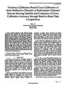
with worldwide coverage. Common satellites with thermal are GOES, MODIS, and Landsat, worldwide coverage. Common satellites with thermal sensorssensors are GOES, MODIS, and Landsat, while while others are country-specific solutions, as CBERS (China-Brazil Earth ResourcesSatellite) Satellite) [10]. [10]. others are country-specific solutions, suchsuch as CBERS (China-Brazil Earth Resources The imagery provided by these satellites ranges from 30 m/pixel/16 days at its finest resolution The imagery provided by these satellites ranges from 30 m/pixel/16 days at its finest resolution (LandsatETM+/TIRS), ETM+/TIRS), to day (VIIRS) toto 500 m/pixel/1 dayday (MODIS Terra/Aqua), to 5 (Landsat to 375 375 m/pixel/1 m/pixel/1 day (VIIRS) 500 m/pixel/1 (MODIS Terra/Aqua), km/pixel/1 day day (GOES). While thethe satellite information is isused surface processes processes to 5 km/pixel/1 (GOES). While satellite information usedfor for large-scale large-scale surface (entirefarm farmto tosub-basin sub-basinand andbasin basinscales), scales),the theinformation informationisisof oflimited limitedvalue valuefor forfine-scale fine-scaleprocesses processes (entire that require requiresub-meter sub-meterscale scalemeasurements measurementsand/or and/or multiple multiple measurements measurements on on the the same same day day (e.g., (e.g., that sunrise, solar noon, mid-afternoon, night). For these requirements, manned aircraft and sUAS sunrise, solar noon, mid-afternoon, night). For these requirements, manned aircraft and sUAS equipped equipped with temperature sensors have Examples been used.ofExamples of airborne and sUAS thermal with temperature sensors have been used. airborne and sUAS thermal applications applications be found Despite in [1,11–23]. Despite its in satellite temperature can be found can in [1,11–23]. its importance in importance satellite temperature related research,related little research, little attention has been paid to atmospheric calibration of thermal imagery from manned attention has been paid to atmospheric calibration of thermal imagery from manned aircraft and aircraftOne andreason sUAS.may Onebe reason mayexpensive be the often expensive meteorological sondes air (to temperature measures air sUAS. the often meteorological sondes (to measures temperature and relative thatalong mustwith be used along with atmospheric profile models such and relative humidity) thathumidity) must be used atmospheric profile models such MODTRAN and MODTRAN and 6S [1,24–30]. By contrast, the technology implemented in manned aircraft/sUAS 6S [1,24–30]. By contrast, the technology implemented in manned aircraft/sUAS (lightweight, relative (lightweight, relative low-cost) thermal is affected by local weather and flightTherefore, elevation low-cost) thermal cameras is affected by cameras local weather and flight elevation conditions. conditions. Therefore, the absence of standards or recommended procedures for referential the absence of standards or recommended procedures for referential calibration and atmospheric calibrationofand atmospheric of thermal cameras for deployment manneduncertainty aircraft or correction thermal cameras correction for deployment on manned aircraft or sUAS can on introduce sUAS can introduce uncertainty andcollect systematic erroritsinsynergistic the data they and limitwith its synergistic and systematic error in the data they and limit use collect in combination available use in combination with available satellite thermal imagery. The objective of this study was to satellite thermal imagery. The objective of this study was to develop standard procedures for vicarious develop standard proceduresflight-specific, for vicarious (sUAS-specific, time-specific, flight-specific, sensor(sUAS-specific, time-specific, and sensor-specific) atmospheric calibrationand of thermal specific) atmospheric calibration of thermal cameras used in sUAS platforms. cameras used in sUAS platforms. 1.1. 1.1.Microbolometers MicrobolometersUAS UASTemperature TemperatureCameras Cameras In In terms terms of of weight weight limitations, limitations, sUAS sUAS (under (under 25 25 kg) kg) have have only only one one available available radiometric radiometric temperature temperature sensor sensorsolution: solution: microbolometer microbolometer infrared infrared sensors sensors (below (below 200 200 gr), gr), which which have have aatypical typical spectral vanadium oxide (VOx) or or amorphous silicon (A-Si) as spectralresponse responsefrom from~7~7um umtoto~14 ~14um, um,using using vanadium oxide (VOx) amorphous silicon (A-Si) the sensor core [31–33]. Figure 1 shows a microbolometer camera as the sensor core [31–33]. Figure 1 shows a microbolometer camerathat thatisissuitable suitablefor forthermal thermalremote remote sensing sensingapplications, applications,as aswell wellas asthe thespectral spectralresponse responseof ofthe thesensor. sensor.Microbolometer Microbolometertechnology technologyuses uses the theresponsiveness responsivenessof ofthe thesensor sensorcore corematerial materialto tochanges changesin insurface surfacetemperature temperaturethat thatare arelarger largerthan than those those of ofthe thesensor sensoritself itself[31]. [31]. These These sensors sensors are arean analternative alternativeto tothe thecryogenically cryogenicallycooled cooledthermal thermal technology technology used usedin inNASA NASAand andESA ESAsatellites satellites[34–36]. [34–36].Miniaturized Miniaturizedcryogenic cryogenictemperature temperaturesensors sensors exist,but butare arestill still heavy sUAS (over 4.0 [37]; Kg) thus, [37]; they thus,are they aremainly used mainly for manned exist, tootoo heavy for for sUAS (over 4.0 Kg) used for manned aircraft. aircraft. The manufacturer’s absolute radiometric calibration playsrole a major role in datawith quality, with The manufacturer’s absolute radiometric calibration plays a major in data quality, reported reported laboratory of ±5 °C (FLIR) ±°C (ICI).1Figure shows the specifications of laboratory accuraciesaccuracies of ±5 ◦ C (FLIR) [37] and [37] ±◦ Cand (ICI). Figure shows1the specifications of an ICI an ICI microbolometer with a spectral typical spectral response microbolometer camera camera with a typical response [38]. [38].
(a)
(b)
Figure 1. Example of the dimensions of a microbolometer ICI Camera 9640 Series, used in this study Figure 1. Example of the dimensions of a microbolometer ICI Camera 9640 Series, used in this study (a). VOx Spectral Response in the 7 to 14 μm Filter, Landsat 8 Band 10 spectral response and average (a). VOx Spectral Response in the 7 to 14 µm Filter, Landsat 8 Band 10 spectral response and average atmospheric transmissivity in the long infrared region (b). atmospheric transmissivity in the long infrared region (b).
Sensors 2017, 17, 1499
3 of 17
1.2. Atmospheric Correction of Surface Temperature All imaging sensors are affected by atmospheric conditions, as indicated by the atmospheric correction models available for the optical and thermal sensors in satellites such as Landsat, Sentinel-3, MODIS, and others [25,27,39–41]. For temperature sensors, the largest sources of distortion are water content in the atmospheric path between the sensor and the surface, in addition to sensor technology and payload integration (i.e., the unit’s accuracy and camera attachment options such as gimbal or frame fitting with/without casing, etc.). For temperature-capable satellites, solutions include an onboard thermal blackbody [27] with a gas-coolant or cryogenic sensor design [42] and minimization of temperature waveband(s) [43] (Figure 1, Landsat 8 spectral response). Nevertheless, these solutions are not available for microbolometer temperature technology (under 200 gr). It is important to compare the spectral response from microbolometer technology for satellites against the atmospheric transmission on the spectral wavebands used to measure surface temperature (7 to 14 um). In this spectral region, water vapor and atmospheric gasses will differentially affect the transmissivity per wavelength and use narrow wavebands: between 8 and 9, and between 10.5 and 12 µm is recommended. However, current microbolometer technology cannot selectively access these recommended narrow wavebandsbecause the technology itself would decrease the sensing capability of the microbolometer with a narrow band (signal to noise ratio) [38]. For satellites and sUAS, the temperature sensor observes the radiation originally emitted from the surface (LG ), but reduced or attenuated by atmospheric factors such as the amount of water vapor and other gasses in the atmosphere column between the ground and the sensor, along with weather conditions, sensor view geometry, etc. The measured radiation at the temperature sensor is called “radiance at sensor” (LS ). The radiation at ground and sensor levels, along with the atmospheric conditions between the sensor and the ground, can be related by using a radiative transfer model [25,44] as presented in Equation (1): LS = τ ε LG + LU + (1 − ε) LD (1) where τ is the atmospheric transmissivity, ε is the emissivity of the surface, LG is the radiance of a blackbody target of kinetic temperature T at ground level, LU is the upwelling or atmospheric path radiance, LD is the downwelling or sky radiance, and LS is the radiance measured by the temperature sensor on board the satellite or manned/sUAS. Radiance is in units of W/m2 /sr/µm, and τ and ε do not have dimensions. If only brightness or radiometric temperature is required, ε can be considered as 1.0, simplifying Equation (1) to Equation (2): LS = τ LG + LU
(2)
For satellite sensors, LU and τ can be determined for the specific image date using a radiative transfer model such as MODTRAN [25,45,46] and 6SV [28–30,47] to calculate the scattering and transmission of radiance through the entire earth atmosphere. These models are time-consuming and require input data that is not often available, such as the vertical profile of atmospheric water vapor and other gasses [1]. The quantification of atmospheric water vapor is needed because, while the atmosphere is a mix of gases (nitrogen, oxygen, carbon dioxide, etc.), these can be considered to be present in constant quantities (with resulting constant effect), but water vapor changes continuously in time and space [48]. To determine the radiance of an object from temperature measurements, Planck’s Law allows the nonlinear relationship of the total emittance as a blackbody, at a specific wavelength, to be determined from its temperature and vice versa [49]. When expressed per unit wavelength, the simplified form of Planck’s Law is Equation (3): W(λ,T) = c1 (λ5 (exp(c2 (λ × T)−1 ) − 1)−1
(3)
where W(λ, T) is the total spectral radiant emittance at a temperature per unit area of emitting surface at wavelength (λ) in meters (W·m−2 ·sr−1 ·um−1 ), T is the temperature in Kelvins, c1
Sensors 2017, 17, 1499
4 of 17
is 1.1910 × 10⁻²² W·m−2 ·µm−1 ·sr−1 , and c2 is 1.4388 × 10⁻² m·K. To obtain surface brightness Sensors 2017, 17, 1499 4 of 16 temperature (without emissivity correction) the equation is inverted as follows to Equation (4): 5 5W) −−1 1 ) − 1)−1−1 T(λ,W) c2(λ ln(c 1(λW) T(λ,W) = c=2 (λ × ×ln(c − 1) 1 (λ
(4) (4)
Equations (3) and (4) use the weighted band center from the specific spectral response of the Equations (3) and (4) use the weighted band center from the specific spectral response of the sensor [1]. It is important to note the linear relationship among the radiance at ground and sensor sensor [1]. It is important to note the linear relationship among the radiance at ground and sensor levels in Equations (1) and (2), while Equations (3) and (4) indicate a nonlinear relationship between levels in Equations (1) and (2), while Equations (3) and (4) indicate a nonlinear relationship between temperature and radiance. temperature and radiance. 2. Materials 2. Materials and and Methods Methods 2.1. Study Site ◦ 170 7.4000 N, is aa commercial commercial vineyard vineyard near near Galt, Galt, CA CA (field (field center center located located at at 38 38°17′7.40′′ The study area is ◦ 60 58.1100 W), 121°6′58.11′′ The farm is equipped with a drip irrigation system and 121 W),operated operatedby byE&J E&JGallo Gallo[50]. [50]. The farm is equipped with a drip irrigation system covers an area of approximately 77 hectares (188 (188 acres). Figure 2 shows the location of theoffarm. The and covers an area of approximately 77 hectares acres). Figure 2 shows the location the farm. location is also an intensive experimental field byby the Sensing The location is also an intensive experimental field theUSDA-ARS USDA-ARSHydrological Hydrologicaland and Remote Remote Sensing Laboratory—GRAPEX (Grape (Grape Remote Remote Sensing Laboratory—GRAPEX Sensing Atmospheric Atmospheric Profiling Profiling and and Evapotranspiration Evapotranspiration Project). Project).
(a)
(b)
(c)
Figure 2. Location of the study area: County location in California (a); AggieAir sUAS coverage area Figure 2. Location of the study area: County location in California (a); AggieAir sUAS coverage area in in RGB mosaic for all flights (b); and close view of sUAS RGB mosaic along with ground temperature RGB mosaic for all flights (b); and close view of sUAS RGB mosaic along with ground temperature sampling locations locations (dots) (dots) (c). (c). sampling
2.2. AggieAir sUAS 2.2. AggieAir sUAS The AggieAir sUAS platforms and payloads developed by Utah State University have been The AggieAir sUAS platforms and payloads developed by Utah State University have been widely widely used for remote sensing assignments in support of research in natural resources, water used for remote sensing assignments in support of research in natural resources, water resources, and resources, and agricultural applications. The system incorporates a collection of sUAS remote sensing agricultural applications. The system incorporates a collection of sUAS remote sensing equipment, equipment, including multiple platforms and interchangeable sensor packages. The customizable including multiple platforms and interchangeable sensor packages. The customizable payload includes payload includes short, medium, and long waveband sensors. The extended flight times of AggieAir short, medium, and long waveband sensors. The extended flight times of AggieAir platforms have platforms have incorporated continuous improvements (3.0 h on a single battery charge, up to 12,000 ft incorporated continuous improvements (3.0 h on a single battery charge, up to 12,000 ft MSL, weather MSL, weather sensors, etc.). To achieve scientific accuracy, intensive ground data collection efforts sensors, etc.). To achieve scientific accuracy, intensive ground data collection efforts have been have been conducted to produce reflectance estimation protocols, address camera vignetting, assure conducted to produce reflectance estimation protocols, address camera vignetting, assure accurate accurate image orthorectification, etc. In addition, the optical and thermal cameras are located within image orthorectification, etc. In addition, the optical and thermal cameras are located within a payload a payload frame to minimize atmospheric effects (chilling) on the sensor due to flight elevations (up frame to minimize atmospheric effects (chilling) on the sensor due to flight elevations (up to 1000 m to 1000 m above ground) and speeds (~50 mph). Figure 3 shows details of the AggieAir “Minion” sUAS and payloads used in this study.
Sensors 2017, 17, 1499
5 of 17
above ground) and speeds (~50 mph). Figure 3 shows details of the AggieAir “Minion” sUAS and payloads used in this study. Sensors 2017, 17, 1499 5 of 16
(a)
(b)
Figure 3. An example of the AggieAir “Minion” sUAS Fixed Wing Aircraft (a); and AggieAir custom Figure 3. An example of the AggieAir “Minion” sUAS Fixed Wing Aircraft (a); and AggieAir custom payload detail (b). payload detail (b).
2.3. Methods 2.3. Methods To develop a vicarious calibration procedure for a microbolometer sensor, the AggieAir sUAS To develop a vicarious calibration procedure for a microbolometer sensor, the AggieAir sUAS was employed to fly over the area of study and collect thermal imagery during a 3-year campaign was employed to fly over the area of study and collect thermal imagery during a 3-year campaign (2014–2016) in agricultural lands (vineyards) in California (Figure 2). Temperature information was (2014–2016) in agricultural lands (vineyards) in California (Figure 2). Temperature information was collected at ground level during each sUAS flight. The flight altitude was 450 m above ground level collected at ground level during each sUAS flight. The flight altitude was 450 m above ground (AGL) and was constant for all flights. Measurements (and flights) were made at early morning level (AGL) and was constant for all flights. Measurements (and flights) were made at early (approximately a half-hour after sunrise), Landsat 8 overpass time (close to solar noon), and midmorning (approximately a half-hour after sunrise), Landsat 8 overpass time (close to solar noon), and afternoon. The AggieAir sUAS navigated over the area of interest based on a pre-programmed flight mid-afternoon. The AggieAir sUAS navigated over the area of interest based on a pre-programmed plan with total flight times of less than 30 min. flight plan with total flight times of less than 30 min. The thermal cameras included in this study are described in Table 1. Both microbolometer The thermal cameras included in this study are described in Table 1. Both microbolometer cameras cameras were acquired from ICI [38]. These instruments were selected partly on the basis of their were acquired from ICI [38]. These instruments were selected partly on the basis of their reported reported laboratory calibration accuracy and ease of integration with the AggieAir payload [38]. In laboratory calibration accuracy and ease of integration with the AggieAir payload [38]. In addition, addition, cameras from this manufacturer have been used by other research groups mentioned in the cameras from this manufacturer have been used by other research groups mentioned in the scientific scientific literature [51–54]. A National Institute of Standards and Technology NIST traceable literature [51–54]. A National Institute of Standards and Technology NIST traceable temperature temperature camera calibration ambient blackbody was acquired from Palmer Wahl [55]. The camera calibration ambient blackbody was acquired from Palmer Wahl [55]. The “ambient” notation “ambient” notation indicates that the blackbody can be used in exterior locations and it does not indicates that the blackbody can be used in exterior locations and it does not require cryogenic or require cryogenic or external cooling for absolute temperature measurement. Table 1 specifies the external cooling for absolute temperature measurement. Table 1 specifies the technical characteristics technical characteristics of the temperature instruments used in this study. of the temperature instruments used in this study. Table 1. Instruments used to collect temperature information in this study. Table 1. Instruments used to collect temperature information in this study.
Instrument Blackbody 2014 2015–2016 Instrument Blackbody 2014 2015–2016 Brand/Model Wahl Palmer/WD1042 ICI/7640-P ICI/9640-P Brand/Model Wahl Palmer/WD1042 ICI/7640-P ICI/9640-P Weight (gr) 1000 148 141 (gr) ImageWeight Size (pixel) --1000 640 by 148 480 640 by141 480 Image Size (pixel) – 640 by 480 640 by 480 Spectral Range (μm) -7 to 14 7 to 14 Spectral Range (µm) – 7 to 14 7 to 14 Spectral Band Centre Spectral Band Centre (µm) – 10.35 10.35 -10.35 10.35 (μm) Range Operating −40 to 70 ◦ C −20 to 100 ◦ C −40 to 140 ◦ C ◦C ◦ C or ± 1.0% ◦C Reported Accuracy ±0.2 ±1.0 ±1.0 Operating Range −40 to 70 °C −20 to 100 °C −40 to 140 °C Reported Emissivity 0.95 ± 0.02 Reported Accuracy ±0.2 °C ±1.0 °C or 1.0 ± 1.0% ±1.0 1.0 °C NIST Traceable? YES NOT REPORTED NOT REPORTED Reported Emissivity 0.95 ± 0.02 1.0 1.0 NIST Traceable? YES NOT REPORTED NOT REPORTED For this study, the AggieAir sUAS was equipped with visual, near-infrared, and thermal cameras. It was flown thethe study area on four dates and times (earlynear-infrared, morning, Landsat For this over study, AggieAir sUASdifferent was equipped with visual, and overpass thermal cameras. It was flown over the study area on four different dates and times (early morning, Landsat overpass and mid-afternoon) (Table 2). These flights acquired thermal imagery at 60-cm/pixel resolution at an elevation of 450 m (1476 ft.) AGL for less than 30 min flight time. The three daily flight times were selected to compare sUAS information with specialized algorithms for evapotranspiration alongside Landsat satellite imagery, which are not part of this study. Agisoft
Sensors 2017, 17, 1499
6 of 17
and mid-afternoon) (Table 2). These flights acquired thermal imagery at 60-cm/pixel resolution at an elevation of 450 m (1476 ft.) AGL for less than 30 min flight time. The three daily flight times were selected to compare sUAS information with specialized algorithms for evapotranspiration alongside Landsat satellite imagery, which are not part of this study. Agisoft Photoscan software [56] was used to create temperature imagery mosaics, while custom MATLAB code and ground control points collected with an RTK GPS system [57] were used to orthorectify the AggieAir imagery [11]. Table 2. AggieAir sUAS flights included in this study (Times in Pacific Daylight Time zone). Early Morning Flights
Date 09 August 2014 02 June 2015 11 July 2015 02 May 2016 03 May 2016
Launch
Landing
7:10 AM 6:51 AM 6:37AM 8:13 AM 8:40 AM
7:30 AM 7:32 AM 7:11 AM 8:35 AM 9:06 AM
Landsat Overpass Flights Launch
Landing
11:30 AM 11:50 AM 11:21 AM 12:06 PM 11:26 AM 12:00 PM 12:53 PM 1:17 PM No UAS flight
Mid-Afternoon Flights Launch
Landing
No UAS flight 2:54 PM 3:20 PM 2:58 PM 3:31 PM 3:52 PM 4:16 PM 1:35 PM 2:00 PM
The vicarious calibration methodology used in this study is initially based on the earlier work by [11], which compared georeferenced ground and sUAS temperature pixels for water pools. The present study considered three major vicarious calibration steps as presented in Table 3. Table 3. Followed vicarious calibration methodology used in this study. Steps
Activity Description
Before Flight
• Camera—blackbody temperature measurement • GPS survey of ground temperature sampling locations
During Flight
• Temperature ground sampling
After Flight
• Ground/sUAS temperature pixel extraction • Calibration of Radiative Transfer Model • sUAS temperature image correction
The three main steps of the vicarious calibration methodology (Table 3) are as follows: •
Before Flight
Two activities had to be accomplished before the flight: (1) a measurement of the ambient temperature blackbody using the sUAS and ground temperature cameras, and (2) a selection and RTK-GPS survey of the locations to be used for ground data collection during the sUAS flight. The first activity allowed the bias to be determined between the temperature cameras and a NIST-traceable instrument. Given that both instruments include reported accuracies, this activity also allowed the bias source (e.g., instrument or environmental) to be determined [58]. The second activity identified areas of interest in the area of study. In agricultural lands, for example, a range of locations was considered that included bare soil (wet and dry), short vegetation (green, dry), tall canopy, and open water surface. The sub-meter pixel resolution of the sUAS thermal images made it necessary to establish the selected locations with temporary or permanent ground markers and perform GPS surveys with sub-centimeter accuracy, thus the need for RTK-GPS equipment. •
During Flight
The previously selected locations were measured with a ground level temperature camera simultaneously with the sUAS flight over the study area. It was important to complete the sUAS flight and the ground data collection in a short amount of time, generally much less than 30 min. This was
Sensors 2017, 17, 1499
7 of 17
to avoid the introduction of measurement errors due to diurnal surface temperature changes. A tall, portable frame was erected on a truck to enable a large number of ground temperature images (and pixels) to be collected quickly. •
After Flight
After the sUAS and ground temperature data were collected, the sUAS temperature map was developed using Sensors 2017, 17, 1499mosaicking software (Agisoft Photoscan) and custom MATLAB code to georeference 7 of 16 the temperature images from the ground data collection. Temperature pixels were then extracted from both the ground andthe sUAS images the resolution the sUAS image. data was extracted from both ground andatsUAS images atof the resolution of theTemperature sUAS image.pixel Temperature then into transformed radiance using Equation (3),using and the radiometric model by [25,44]) pixeltransformed data was then into radiance Equation (3), and the(proposed radiometric model shown in Equation (2) was applied. Finally, atmospheric transmissivity and atmospheric path radiance (proposed by [25,44]) shown in Equation (2) was applied. Finally, atmospheric transmissivity and were applied to the radiance entire sUAS radiance image (converted from aradiance temperature map) and transformed atmospheric path were applied to the entire sUAS image (converted from a back into an atmospherically corrected temperature image. temperature map) and transformed back into an atmospherically corrected temperature image. 3. 3. Results Results and and Discussion Discussion 3.1. 3.1. Before Before Flight Flight Camera–Blackbody total of of 213 213 individual individual temperature temperature Camera–Blackbody Temperature Temperature Imagery Imagery Measurement: Measurement: A A total images of the blackbody were compared to determine bias in the microbolometer cameras usedused in this images of the blackbody were compared to determine bias in the microbolometer cameras in 3-year study. Figure 4 shows an example of the visual and temperature images of the NIST-traceable this 3-year study. Figure 4 shows an example of the visual and temperature images of the NISTambient blackbodyblackbody in the field. traceabletemperature ambient temperature in the field.
(a)
(b)
Figure 4. Visual (a) and temperature (b) images of the NIST traceable ambient temperature blackbody Figure 4. Visual (a) and temperature (b) images of the NIST traceable ambient temperature blackbody used in this study. Black disk (a) is the blackbody temperature sensor. used in this study. Black disk (a) is the blackbody temperature sensor.
As specified in Table 1, the temperature blackbody works at an emissivity value of 0.95 ± 0.02, As specified in Table 1,camera the temperature at an emissivity value oftemperature 0.95 ± 0.02, while the microbolometer worked atblackbody a value ofworks 1.0. Therefore, the blackbody while the microbolometer camera worked at a value of 1.0. Therefore, the blackbody temperature was was adjusted to the camera emissivity using the Stefan-Boltzmann Law (5): adjusted to the camera emissivity using the Stefan-Boltzmann Law (5): Tblackbody·corrected4 = (εblacbody/εcamera) × Tblackbody4 (5) 4 4 T = (εblacbody /εcamera ) × Tblackbody (5) ·corrected adjusted where Tblackbody corrected isblackbody the emissivity temperature, εcamera (1.0) and εblackbody (0.95) are the emissivities of the microbolometer cameras and the blackbody, respectively, and Tblackbody is the where Tblackbody corrected is the emissivity adjusted temperature, εcamera (1.0) and εblackbody (0.95) are temperature reported by the ambient blackbody. Once the blackbody temperature was corrected for the emissivities of the microbolometer cameras and the blackbody, respectively, and Tblackbody is the emissivity, the temperatures (blackbody and cameras) were modeled as shown in Figure 5. In temperature reported by the ambient blackbody. Once the blackbody temperature was corrected for addition, a sensitivity analysis of the camera and blackbody instrument accuracies (Table 1) were performed. As shown in Figure 5 and Table 4, a strong linear relationship exists between the data from the microbolometer cameras provided by ICI and the ambient blackbody. The linear response to a 1:1-line slope indicates that the ICI microbolometer cameras needed only a constant bias correction expressed by an independent term (−2.67 °C) in the equation shown in Figure 5a. The relationship thus identified
Sensors 2017, 17, 1499
8 of 17
emissivity, the temperatures (blackbody and cameras) were modeled as shown in Figure 5. In addition, a sensitivity analysis of the camera and blackbody instrument accuracies (Table 1) were performed. As shown in Figure 5 and Table 4, a strong linear relationship exists between the data from the microbolometer cameras provided by ICI and the ambient blackbody. The linear response to a 1:1-line slope indicates that the ICI microbolometer cameras needed only a constant bias correction expressed by an independent term (−2.67 ◦ C) in the equation shown in Figure 5a. The relationship thus identified was not affected by weather conditions or seasonality (air temperature, wind, humidity, etc.). In addition, Figure 5b shows a residual analysis of the camera-blackbody linear model. The bias residuals have a distribution similar to a Gaussian curve (mean = 0.0 ◦ C, and standard deviation ±1.22 ◦ C). In addition, up to 48% of the residual variability around the mean can be explained by the accuracy of17, the blackbody (±0.2 ◦ C, ±0.02 ε or ±0.35 ◦ C when both accuracies are combined), and Sensors 2017, 1499 8 ofup 16 to 68% of the residual variability around the mean is explained by the accuracy of the thermal camera (Therefore, ±1.00 ◦ C). 32% Therefore, of the variability in the residuals the modeled bias seemed be caused of the32% variability in the residuals of the of modeled bias seemed to betocaused by by measurement factors (e.g., optical characteristicsofofthe theICI ICIcamera camerasuch suchas asthe thepoint point spread spread function measurement factors (e.g., optical characteristics and selection of blackbody pixels from from the the temperature temperature image). image).
(a)
(b)
Figure 5. Temperature camera–blackbody comparison for 213 individual measurements. A linear Figure 5. Temperature camera–blackbody comparison for 213 individual measurements. A linear model with a unit slope (1:1) and a constant bias (−2.67 °C) fitted the camera bias value over 3 years model with a unit slope (1:1) and a constant bias (−2.67 ◦ C) fitted the camera bias value over 3 years of study. Temperature values below 30 °C for the ground camera axis belong to early morning of study. Temperature values below 30 ◦ C for the ground camera axis belong to early morning measurements, higher values are for Landsat overpass and mid-afternoon times (a); Reported measurements, higher values are for Landsat overpass and mid-afternoon times (a); Reported accuracies accuracies from blackbody and camera manufacturers can explain up to 48% (gray region) and 68% from blackbody and camera manufacturers can explain up to 48% (gray region) and 68% (orange region) (orange region) of linear model residuals variability, respectively (b). of linear model residuals variability, respectively (b). Table 4. Statistics camera—blackbody linear linear model model analysis. analysis. Table 4. Statistics for for Temperature Temperature camera—blackbody
Slope (95% Slope (95% Confidence Model Confidence Bounds) Bounds) Linear 1.00 (0.99 1.02)
Model
Linear
1.00 (0.99 1.02)
Reported Bias (95% Reported RMSE Reported Reported Confidence R2 2 Blackbody Bias (95% RMSE Camera Camera Blackbody R (C°) ◦ Confidence (C ) Accuracy (C°) ◦ Accuracy (C°) Bounds)Bounds) Accuracy (C ) Accuracy (C◦ ) −2.67 (−3.19 − 2.22) 0.99 1.23 ±1.00 ±0.35 −2.67 (−3.19–2.22)
0.99
1.23
±1.00
±0.35
Ground temperature sampling locations: Different land surfaces were considered during the Ground temperature sampling locations: surfacessurface were considered during the three-year data collection effort for this project. Different Examplesland of different types are presented in three-year data collection effort for this project. Examples of different surface types are presented in Figures 2 and 6. These locations were visually homogeneous and covered the range of possible land Figures and These homogeneous covered the range made of possible land surfaces2in the6.area of locations study. Anwere RTKvisually GPS system was usedand to survey perimeters with PVC surfaces in the area of study. An RTK GPS system was used to survey perimeters made with PVC and and aluminum tape (1.6 by 1.6 m and 0.8 by 0.8 m) so that sUAS and ground temperature pixels could aluminum tape (1.6 by 1.6 m and 0.8 by 0.8 m) so that sUAS and ground temperature pixels could be be accurately located. accurately located.
Ground temperature sampling locations: Different land surfaces were considered during the three-year data collection effort for this project. Examples of different surface types are presented in Figures 2 and 6. These locations were visually homogeneous and covered the range of possible land surfaces in the area of study. An RTK GPS system was used to survey perimeters made with PVC and aluminum tape (1.6 by 1.6 m and 0.8 by 0.8 m) so that sUAS and ground temperature pixels could Sensors 2017, 17, 1499 9 of 17 be accurately located.
(a)
(b)
(c)
Figure 6. Examples of ground locations for temperature sampling the day before the sUAS flight Figure 6. Examples of ground locations for temperature sampling the day before the sUAS flight shown shown in2.Figure 2. Locations were delimited using PVC and using surveyed RTK the GPS. Note the in Figure Locations were delimited using PVC and surveyed RTK using GPS. Note diversity of diversity of locations: bare dry soil (a), short green canopy (b), and tall canopy (c). locations: bare dry soil (a), short green canopy (b), and tall canopy (c).
Sensors 2017, 17, 1499
9 of 16
3.2.During DuringFlight Flight 3.2. Temperature Ground Ground Sampling: Sampling: Simultaneous Simultaneous examples examples of of AggieAir AggieAirsUAS sUASflights flightsand andground ground Temperature temperature captures captures are are presented presented in in Figure Figure 7: 7: temperature
(a)
(b)
(c)
Figure 7. An example of ground temperature samples taken using the temperature camera mounted Figure 7. An example of ground temperature samples taken using the temperature camera mounted on height) and connected to atolaptop loaded withwith ICI software IR FLASH on 3 May onaatripod tripod(3(3mm height) and connected a laptop loaded ICI software IR FLASH on 32016, May at Landsat overpass time. Temperature images of the top of vine canopy (a) and bare 2016, at Landsat overpass time. Temperature images of the top of vine canopy (a) and baresoil soil(b). (b). Temperature temperature sampling sampling (c). (c). Temperature camera camera and and tripod tripod mounted mounted over over aa truck truck for for fast fast ground ground temperature
3.3. After Flight 3.3. After Flight Ground and sUAS Pixel Extraction: After each flight, sUAS temperature maps were developed Ground and sUAS Pixel Extraction: After each flight, sUAS temperature maps were developed using data from the sUAS onboard inertial measurement unit (IMU) and GPS receiver. This provided using data from the sUAS onboard inertial measurement unit (IMU) and GPS receiver. This provided the sUAS location (x, y, z coordinates) and orientation (pitch, roll, yaw) to the Agisoft Photoscan the sUAS location (x, y, z coordinates) and orientation (pitch, roll, yaw) to the Agisoft Photoscan version 1.3 software [56]. RTK-GPS surveyed ground control points, specifically for thermal cameras version 1.3 software [56]. RTK-GPS surveyed ground control points, specifically for thermal cameras (aluminum-based blankets), were also included. For the ground temperature camera images, these (aluminum-based blankets), were also included. For the ground temperature camera images, these points were registered using their respective RTK-GPS coordinates and ground PVC frame points were registered using their respective RTK-GPS coordinates and ground PVC frame dimensions dimensions using ESRI ArcGIS software. An example of georeferenced ground temperature images using ESRI ArcGIS software. An example of georeferenced ground temperature images is shown in is shown in Figure 8. Figure 8.
Figure 8. Example of ground temperature images georeferenced from locations shown in Figure 6
the sUAS location (x, y, z coordinates) and orientation (pitch, roll, yaw) to the Agisoft Photoscan version 1.3 software [56]. RTK-GPS surveyed ground control points, specifically for thermal cameras (aluminum-based blankets), were also included. For the ground temperature camera images, these points were registered using their respective RTK-GPS coordinates and ground PVC frame dimensions using ESRI ArcGIS software. An example of georeferenced ground temperature images Sensors 2017, 17, 1499 10 of 17 is shown in Figure 8.
Figure 8. Example of ground temperature images georeferenced from locations shown in locations Figure 6 and Figure 8. Example of ground temperature images georeferenced from shown in Figure 6 others over a visual image over usinga ArcGIS. The figure thermal imagestemperature of two and others visual image using showcases ArcGIS. The figure temperature showcases thermal images of bare soil locations (top) and two tall canopies (vines) (bottom). Square grids indicate sUAS and ground two bare soil locations (top) and two tall canopies (vines) (bottom). Square grids indicate sUAS and pixels that can be extracted forthat atmospheric radiance ground pixels can be extracted forcalibration. atmospheric radiance calibration.
of Radiance Atmospheric Radiance Once extracted, from the sUAS thermal Calibration ofCalibration Atmospheric Model: Once Model: extracted, data from thedata sUAS thermal images and ground temperature values were transformed into radiance Equation (3). The images and ground temperature values were transformed into radiance Equation (3). The atmospheric atmospheric radiance model presented in Equation wasflight, calibrated for results every sUAS radiance model presented in Equation (2) was calibrated for every(2) sUAS and the of theflight, and the results of the calibration are shown in Table 5. Figure 9 shows the radiance comparison calibration are shown in Table 5. Figure 9 shows the radiance comparison from sUAS and ground pixels. from sUAS and ground pixels. Table 5. Statistical results from atmospheric radiance model (τ and Lu) using ground and sUAS pixels. Date 8/9/2014
6/2/2015
7/11/2015
5/2/2016
5/3/2016
Flight Time
τ (95% Confidence Bounds)
Lu (95% Confidence Bounds) W/m2 /µm/sr
r2
RMSE W/m2 /µm/sr
Used Pixels
Early Morning
0.40 (0.51 0.33)
−5.54 (−9.38–3.03)
0.65
0.37
48
Landsat Overpass
0.69 (0.88 0.57)
−2.94 (−6.75–0.45)
0.58
0.84
63
Early Morning
0.35 (0.38 0.33)
−4.28 (−5.10–3.56)
0.71
0.26
336
Landsat Overpass
0.57 (0.62 0.53)
−3.61 (−4.88–2.53)
0.62
0.88
330
Mid Afternoon
0.53 (0.58 0.50)
−5.17 (−6.49–4.04)
0.68
0.97
330
Early Morning
0.81 (0.88 0.76)
−0.94 (−1.58–0.39)
0.73
0.12
283
Landsat Overpass
0.49 (0.52 0.47)
−5.08 (−5.86–4.38)
0.83
0.77
352
Mid Afternoon
0.47 (0.48 0.45)
−5.21 (−5.71–4.74)
0.94
0.47
278
Early Morning
0.29 (0.33 0.27)
−5.23 (−6.66–4.05)
0.53
0.21
343
Landsat Overpass
0.62 (0.63 0.60)
−2.21 (−2.49–1.94)
0.95
0.46
299
Mid Afternoon
0.65 (0.69 0.62)
−2.25 (−2.94–1.62)
0.79
0.55
299
Early Morning
0.43 (0.45 0.41)
−4.74 (−5.49–4.07)
0.8
0.13
326
Mid Afternoon
0.52 (0.55 0.50)
−3.38 (−4.01–2.82)
0.83
0.43
349
In Figure 9 and Table 5 the Equation (2) linear model assumption is confirmed by the linearity of the ground and sUAS pixel comparison. Not all Equation (4) regression calibrations (Table 5) have a high R2 value, due to the scattering of the compared pixels, but small average errors (RMSE) were observed for early morning (