Mar 24, 2017 - and Live TV Content from cloud servers have been studied ...... [9] B. Han, F. Qian, L. Ji, V. Gopalakrishnan, and N. Bedminster, âMp-.
1
Video Streaming in Distributed Erasure-coded Storage Systems: Stall Duration Analysis
arXiv:1703.08348v1 [cs.NI] 24 Mar 2017
Abubakr O. Al-Abassi and Vaneet Aggarwal
Abstract—The demand for global video has been burgeoning across industries. With the expansion and improvement of videostreaming services, cloud-based video is evolving into a necessary feature of any successful business for reaching internal and external audiences. This paper considers video streaming over distributed systems where the video segments are encoded using an erasure code for better reliability thus being the first work to our best knowledge that considers video streaming over erasure-coded distributed cloud systems. The download time of each coded chunk of each video segment is characterized and ordered statistics over the choice of the erasure-coded chunks is used to obtain the playback time of different video segments. Using the playback times, bounds on the moment generating function on the stall duration is used to bound the mean stall duration. Moment generating function based bounds on the ordered statistics are also used to bound the stall duration tail probability which determines the probability that the stall time is greater than a pre-defined number. These two metrics, mean stall duration and the stall duration tail probability, are important quality of experience (QoE) measures for the end users. Based on these metrics, we formulate an optimization problem to jointly minimize the convex combination of both the QoE metrics averaged over all requests over the placement and access of the video content. The non-convex problem is solved using an efficient iterative algorithm. Numerical results show significant improvement in QoE metrics for cloud-based video as compared to the considered baselines. Index Terms—Distributed Storage, Erasure Codes, Stall Duration, Video Streaming
I. I NTRODUCTION The demands of video streaming services have been skyrocketing over these years, with the global video streaming market expected to grow annually at a rate of 18.3% [1]. With the proliferation and advancement of video-streaming services, cloud-based video has become an imperative feature of any successful business. This can also be seen as IBM estimates cloud-based video will be a $105 billion market opportunity by 2019 [2]. In cloud storage systems, erasure coding has seen itself quickly emerged as a promising technique to reduce the storage cost for a given reliability as compared to the replicated systems [3], [4]. It has been widely adopted in modern storage systems by companies like Facebook [5], Microsoft [6] and Google [7]. This paper considers video streaming when the content is placed on cloud servers, where erasure coding is used. The key quality of experience (QoE) metric for video streaming is the duration of stalls at the clients. This paper gives bounds on the stall durations, and uses that to propose The authors are with the School of Industrial Engineering, Purdue University, West Lafayette IN 47907, email: {aalabbas,vaneet}@purdue.edu. This work was supported in part by the National Science Foundation under Grant no. CNS-1618335.
an optimized streaming service that minimizes average QoE for the clients. In this paper, we consider two measures of QoE metrics in terms of stall duration. The first is the mean stall duration. Almost every viewer can relate to the quality of experiences for watching videos being the stall duration and is thus one of the key focus in the studied streaming algorithms [8], [9]. The second is the probability that the stall duration is greater than a fixed number x, which determines the stall duration tail probability. It has been shown that in modern Web applications such as Bing, Facebook, and Amazon’s retail platform, the long tail of latency is of particular concern, with 99.9th percentile response times that are orders of magnitude worse than the mean [10], [11]. Thus, the QoE metric of stall duration tail probability becomes important. This paper characterizes an upper bound on both the QoE metrics. We note that quantifying service latency for erasure-coded storage is an open problem [12], and so is tail latency [13]. This paper takes a step forward and explores the notions for video streaming rather than video download. Thus, finding the exact QoE metrics is an open problem. This paper finds the bounds on the QoE metrics. The data chunk transfer time in practical systems follows a shifted exponential distribution [14], [15] which motivates the choice that the service time distribution for each video server is a shifted exponential distribution. Further, the request arrival rates for each video is assumed to be Poisson. The video segments are encoded using an (n, k) erasure code and the coded segments are placed on n different servers. When a video is requested, the segments need to be requested from k out of n servers. Optimal strategy of choosing these k servers would need a Markov approach similar to that in [12] and suffers from a similar state explosion problem, because states of the corresponding queuing model must encapsulate not only a snapshot of the current system including chunk placement and queued requests but also past history of how chunk requests have been processed by individual nodes. In this paper, we use the probabilistic scheduling proposed in [14], [16] to access the k servers, where each possibility of k servers is chosen with certain probability and the probability terms can be optimized. Using this scheduling mechanism, the random variables corresponding to the times for download of different video segments from each server are found. Using ordered statistics over the k servers, the random variables corresponding to the playback time of each video segment are characterized. These are then used to find bounds on the mean stall duration and the stall duration tail probability. Moment generating functions of the ordered statistics of different ran-
2
dom variables are used in the bounds. We note that the problem of finding latency for file download is very different from the video stall duration for streaming. This is because the stall duration accounts for download time of each video segment rather than only the download time of the last video segment. Further, the download time of segments are correlated since the download of chunks from a server are in sequence and the playback time of a video segment are dependent on the playback time of the last segment and the download time of the current segment. Taking these dependencies into account, this paper characterizes the bounds on the two QoE metrics. We note that for the special case when each video has a single segment, the bounds on mean stall duration and stall duration tail probability reduce to that for file download. Further, the bounds based on the approach in this paper have been shown to outperform the results for mean file download latency in [14], [16]. The proposed framework provides a mathematical crystallization of the engineering artifacts involved and illuminates key system design issues through optimization of QoE. The average QoE metric over different requests can be optimized over the placement of the video files, the access of the video files from the servers, and the bound parameters. The tradeoff in the two QoE metrics is captured by defining the objective function which is a convex combination of the two QoE metrics. Varying the parameter trading off the two metrics can be used to get a tradeoff region between the two metrics helping the system designer to choose an appropriate point. An efficient algorithm is proposed to solve the proposed nonconvex problem. The proposed algorithm does an alternating optimization over the placement, access, and the bound parameters. The optimization over probabilistic scheduling access parameters help reduce the mean and tail of the stall durations by differentiating video files thus providing more flexibility as compared to choosing the lowest queue servers. The sub-problems have been shown to have convex constraints and thus can be efficiently solved using iNner cOnVex Approximation (NOVA) algorithm proposed in [17], [18]. The proposed algorithm is shown to converge to a local optimal. Numerical results demonstrate significant improvement of QoE metrics as compared to the baselines. The key contributions of our paper include: This paper formulates video streaming over erasure-coded cloud storage system. • The random variable corresponding to the download time of a chunk of each video segment from a server is characterized. Using ordered statistics, the random variable corresponding to the playback time of each video segment is found. These are further used to derive upper bounds on the mean stall duration of the video and the video stall duration tail probability. • The QoE metrics are used to formulate system optimization problems over the choice of the placement of video segments, probabilistic scheduling access policy and the bound parameters which are related to the moment generating function. Efficient iterative solutions are provided for these optimization problems. •
Numerical results show that the proposed algorithms converges within a few iterations. Further, the QoE metrics are shown to have significant improvement as compared to the considered baselines. For instance, the mean stall duration for the proposed algorithm is 60% smaller and the stall duration tail probability is orders of magnitude better as compared to random placement and projected equal access probability strategy. The remainder of this paper is organized as follows. Section 2 provides related work for this paper. In Section 3, we describe the system model used in the paper with a description of video streaming over cloud storage. Section 4 derives expressions on the download and play times of the chunks which are used in Sections 5 and 6 to find the upper bounds on the QoE metrics of the mean stall duration and video stall latency, respectively. Section 7 formulates the QoE optimization problem as a weighted combination of the two QoE metrics and proposes the iterative algorithmic solution of this problem. Numerical results are provided in Section 8. Section 9 concludes the paper. •
II. R ELATED W ORK Latency in Erasure-coded Storage: To our best knowledge, however, while latency in erasure coded storage systems has been widely studied, quantifying exact latency for erasurecoded storage system in data-center network is an open problem. Prior works focusing on asymptotic queuing delay behaviors [19], [20] are not applicable because redundancy factor in practical data centers typically remains small due to storage cost concerns. Due to the lack of analytic latency models, most of the literature is focused on reliable distributed storage system design, and latency is only presented as a performance metric when evaluating the proposed erasure coding scheme, e.g., [21]–[25], which demonstrate latency improvement due to erasure coding in different system implementations. Related design can also be found in data access scheduling [26]–[28], access collision avoidance [29], [30], and encoding/decoding time optimization [31], [32] and there is also some work using the LT erasure codes to adjust the system to meet user requirements such as availability, integrity and confidentiality [33]. Recently, there has been a number of attempts at finding latency bounds for an erasure-coded storage system [12], [14]– [16], [34], [35]. The key scheduling approaches include blockone-scheduling policy that only allows the request at the head of the buffer to move forward [34], fork-join queue [35], [36] to request data from all server and wait for the first k to finish, and the probabilistic scheduling [14], [16] that allows choice of every possible subset of k nodes with certain probability. Mean latency and tail latency have been characterized in [14], [16] and [13] respectively for a system with multiple files using probabilistic scheduling. This paper considers video streaming rather than file downloading. The metrics for video streaming does not only account for the end of the download of the video but also of the download of each of the segment. Thus, the analysis for the content download cannot be extended to the video streaming directly and the analysis approach in this paper is very different from the prior works in the area.
3
Video i:
Video Streaming over Cloud: Servicing Video on Demand and Live TV Content from cloud servers have been studied widely [37]–[41]. The placement of content and resource optimization over the cloud servers have been considered. To the best of our knowledge, reliability of content over the cloud servers have not been considered for video streaming applications. In the presence of erasure-coding, there are novel challenges to characterize and optimize the QoE metrics at the end user. Adaptive streaming algorithms have also been considered for video streaming [42], [43], which are beyond the scope of this paper and are left for future work. III. S YSTEM M ODEL We consider a distributed storage system consisting of m heterogeneous servers (also called storage nodes), denoted by M = 1, 2, ..., m. Each video file i, where i = 1, 2, ...r, is divided into Li equal segments, Gi,1 , · · · , Gi,Li , each of length τ sec. Then, each segment Gi,j for j ∈ {1, 2, . . . , Li } is partitioned into ki fixed-size chunks and then encoded using an (ni , ki ) Maximum Distance Separable (MDS) erasure code to generate ni distinct chunks for each segment Gi,j . These (1) (n ) coded chunks are denoted as Ci,j , · · · , Ci,ji . The encoding setup is illustrated in Figure 1. The encoded chunks are stored on the disks of ni distinct storage nodes. These storage nodes are represented by a set Si , such that Si ⊆ M and ni = |Si |. Each server z ∈ Si stores (g ) all the chunks Ci,jz for all j and for some gz ∈ {1, · · · , ni }. In other words, each of the ni storage nodes stores one of the coded chunks for the entire duration of the video. The placement on the servers is illustrated in Figure 2, where the server 1 is shown to store first coded chunks of file i, third coded chunks of file u and first coded chunks for file v. The use of (ni , ki ) of MDS erasure code introduces a redundancy factor of ni /ki which allows the video to be reconstructed from the video chunks from any subset of ki out-of-ni servers. Hence, when a video i is requested, the request goes to a set Ai of the storage nodes, where Ai ⊆ Si (g ) and ki = |Ai |. From each server z ∈ Ai , all chunks Ci,jz for all j and the value of gz corresponding to that placed on server z are requested. The request is illustrated in Figure 2. (g ) In order to play a segment q of video i, Ci,qz should have been downloaded from all z ∈ Ai . We note that erasure coding is a generalization of replication with ki = 1 and thus the framework includes the scenario where the files are replicated for reliability rather than erasure-coded. The key used notations are defined in Table I. We assume that the files at each server are served in order of the request in a first-in-first-out (FIFO) policy. Further, the different chunks are processed in order of the duration. This is depicted in Figure 3, where for a server q, when a file i is requested, all the chunks are placed in the queue where other video requests before this that have not yet been served are waiting. In order to schedule the requests for video file i to the ki servers, the choice of ki -out-of-ni servers is important. Finding the optimal choice of these servers to compute the latency expressions is an open problem to the best of our
G i,1 G
(1)
(1)
B i,j
C i,j
(2)
i,2
j th Segment
G i,j
(2)
B i,j
(n i ,k i)
Ci,j
Encoding
(k )
(n )
C i,j i
B i,ji
Gi,L ii
Fig. 1: A schematic illustrates video fragmentation and erasure-coding processes. Video i is composed of Li segments. Each segments is partitioned into ki chunks and then encoded using an (ni , ki ) MDS code. Server 1
Server m
Server 2
(1) (1) C i,1 C i,2
(1) Ci,L i
(5) (5) C i,1 C i,2
C (5) i,Li
(j) (j) C i,1 C i,2
C (j) i,Li
(3) (3) C u,1 Cu,2
C (3) u,Lu
(2) (2) C u,1 Cu,2
C (2) u,Lu
(4) (4) C u,1 Cu,2
C (4) u,Lu
(1) (1) C v,1 Cv,2
C (1) v,Lv
(j) (j) C v,1 Cv,2
C (j) v,Lv
(2) (2) C v,1 Cv,2
C (2) v,Lv
Requests for video i, u, v
Joint Scheduler (K i-out-of-n i)
Fig. 2: An Illustration of a distributed storage system equipped with m nodes and storing 3 video files assuming (ni , ki ) erasure codes. knowledge. Thus, this paper uses a policy, called Probabilistic Scheduling, which was proposed in [14], [16]. This policy allows choice of every possible subset of ki nodes with certain probability. Upon the arrival of a video file i, we randomly dispatch the batch of ki chunk requests to appropriate a set of nodes (denoted by set Ai of servers for file i) with predetermined probabilities (P (Ai ) for set Ai and file i). Then, each node buffers requests in a local queue and processes in order and independently as explained before. The authors of [14], [16] proved that a probabilistic scheduling policy with feasible probabilities {P (Ai ) : ∀i , Ai } exists if and only if there exists conditional probabilities πij ∈ [0, 1] ∀i, j satisfying m X
πij = ki ∀i
and πij = 0 if j ∈ / Si .
j=1
In other words, selecting each node j with probability πij Waiting Queue at Server q (1) (1) C i,1 C i,2
File i
C (1) i,L i
(4) (4) C u,1 C u,2
C (4) u,L u
(2) (2) C v,1 C v,2
C (2) v,L v
Fig. 3: An Example of the instantaneous queue status at server q, where q ∈ 1, 2, ..., m.
4
would yield a feasible choice of {P (Ai ) : ∀i , Ai }. Thus, we consider the request probabilities πij as the probability that the request for video file i uses server j. While the probabilistic scheduling have been used to give bounds on latency of file download, this paper uses the scheduling to give bounds on the QoE for video streaming. We note that it may not be ideal in practice for a server to finish one video request before starting another since that increases delay for the future requests. However, this can be easily alleviated by considering that each server has multiple queues which can all be considered as separate servers. The probabilistic scheduling can choose ki of the overall queues to access the content. Having y queues at each server makes the total number of queues as y × m, and each server can simultaneously service y videos adding flexibility and decreasing the overall stall times. Since this is an easy modification and does not affect the analysis, we assume y = 1 in this paper. We assume a single Virtual Machine (VM) requesting the video files from the servers and the links from the VM to the clients is not considered a bottleneck in this paper. In practice, there may be multiple aggregation VMs serving subsets of clients in which case the problem for each of the aggregation VMs can be made independent in the VMs by controlling the bandwidth resources from the servers to the different VMs. Thus, without loss of generality, this paper considers only one VM representing multiple clients. We now describe a queuing model of the distributed storage system. We assume that the arrival of client requests for each video i form an independent Poisson process with a known rate λi . The arrival of file Prequests at node j forms a Poisson Process with rate Λj = i λi πi,j which is the superposition of r Poisson processes each with rate λi πi,j . We assume that the chunk service time for each coded chunk (g ) Ci,lj at server j, Xj , follows a shifted exponential distribution as has been demonstrated in realistic systems [14], [15]. The service time distribution for the chunk service time at server j, Xj , is given by the probability distribution function fj (x), which is ( αj e−αj (x−βj ) , x ≥ βj fj (x) = . (1) 0, x < βj We note that exponential� distribution is a special case with � βj = 0. Let Mj (t) = E etXj be the moment generating function of Xj . Then, Mj (t) is given as Mj (t) =
αj eβj t αj − t
t < αj
(2)
We note that the arrival rates are given in terms of the video files, and the service rate above is provided in terms of the coded chunks at each server. The client plays the video segment after all the ki chunks for the segment have been downloaded and the previous segment has been played. We also assume that there is a start-up delay of ds (in seconds) for the video which is the duration in which the content can be buffered but not played. This paper will characterize the stall duration and stall duration tail probability for this setting.
TABLE I: Key Notations Used in This Paper Symbol r m Li Gi,j (ni , ki ) (q) Ci,j λi πij Si Ai (αj , βj ) Xj Mj (t) x (q) Di,j Rj Rj Bj (t) µj Λj ρj (q) Ti ds τ Γ(i) θ
Meaning Number of video files in system Number of storage nodes Number of segments for video file i Segment j of video file i Erasure code parameters for file i q th coded chunk of segment j in file i Possion arrival rate of file i Probability of retrieving chunk of file i from node j using probabilistic scheduling algorithm Set of storage nodes having coded chunks of file i Set of storage nodes used to access chunks from file i Parameters of Shifted Exponential distribution Service time distribution of a chunk at node j Moment generating function for� the service time of � a chunk at node j Mj (t) = E etXj Parameter indexing stall duration tail probability Download time for coded chunk q ∈ {1, . . . , Li } of file i from storage node j Service time of the video files Laplace-Stieltjes � �Transform of Rj , Rj = E e−sRj Moment generating function � �for the service time of video files Bj (t) = E etRj Mean service time of a chunk from storage node j Aggregate arrival rate at node j Video file request intensity at node j The time at which the segment Gi,q is played back Start-up delay Chunk size in seconds Stall duration tail probability for file i Trade off factor between mean stall duration and stall duration tail probability
IV. D OWNLOAD AND P LAY T IMES OF THE C HUNKS In order to understand the stall duration, we need to see the download time of different coded chunks and the play time of the different segments of the video. A. Download Times of the Chunks from each Server In this subsection, we will quantify the download time of (g ) chunk for video file i from server j which has chunks Ci,qj (g ) for all q = 1, · · · Li . We consider download of q th chunk Ci,qj . (g ) As seen in Figure 3, the download of Ci,qj consists of two components - the waiting time of all the video files in queue before file i request and the service time of all chunks of video file i up to the q th chunk. Let Wj be the random variable corresponding to the waiting time of all the video files in queue (q) before file i request and Yj be the (random) service time of coded chunk q for file i from server j. Then, the (random) download time for coded chunk q ∈ {1, · · · , Li } for file i at (q) server j ∈ Ai , Di,j , is given as (q)
Di,j = Wj +
q X
(v)
Yj .
(3)
v=1
We will now find the distribution of Wj . We note that this is the waiting P time for the video files whose arrival rate is given as Λj = i λi πi,j . Since the arrival rate of video files is Poisson, the waiting time for the start of video download
5
from a server j, Wj , is given by an M/G/1 process. In order to find the waiting time, we would need to find the service time statistics of the video files. Note that fj (x) gives the service time distribution of only a chunk and not of the video files. Video file i consists of Li coded chunks at server j (j ∈ Si ). The total service time for video file i at server j if requested from server j, STi,j , is given as STi,j =
Li X
(v)
Yj .
(4)
service time is general distributed. Thus, the Laplace-Stieltjes Transform of the waiting time Wj is given as (1 − ρj ) sRj (s) � s − Λj 1 − Rj (s)
� � E e−sWj =
(10)
Having characterized the Laplace-Stieltjes Transform of the (v) waiting time Wj and knowing the distribution of Yj , the (q) Laplace-Stieltjes Transform of the download time Di,j is given as
v=1
The service time of the video files is given as n π λi ∀i, Rj = STi,j with probability ij Λj
(q)
E[e (5)
since the service time is STi,j when file i is requested from server j. Let Rj (s) = E[e−sRj ] be the Laplace-Stieltjes Transform of Rj . Lemma 1. h i The Laplace-Stieltjes Transform of Rj , Rj (s) = −sRj E e is given as Rj (s) =
r X i=1
πij λi Λj
�
−sDi,j
(1 − ρj ) sRj (s) � ]= s − Λj 1 − Rj (s)
(6)
αj e−βj s αj + s
�q . (11)
We note that the expression � above holds only in the range of s when s−Λj 1 − Rj (s) > 0 and αj +s > 0. Further, the server utilization ρj must be less than 1. The overall download (q) time of all the chunks for the segment Gi,q at the client, Di , is given by (q)
Di
� −βj s Li
αj e αj + s
�
(q)
= max Di,j .
(12)
j∈Ai
B. Play Time of Each Video Segment (q)
Let Ti be the time at which the segment Gi,q is played (started) at the client. The startup delay of the video is ds . Then, the first segment can be played at the maximum of the time the first segment can be downloaded and the startup delay. Thus,
Proof. Rj (s) =
r X πij λi i=1 r X
Λj
h i E e−s(STi,j )
� �PL �� (ν) i πij λi −s ν=1 Yj E e Λj i=1 r X πij λi � � −s�Y (1) � ��Li j = E e Λj i=1 � �Li r X πij λi αj e−βj s = Λj αj + s i=1 =
(1)
Ti
(7)
Corollary 1. The moment generating function for the service time of video files when requested from server j, Bj (t), is given by � �Li r X πij λi αj eβj t (8) Bj (t) = Λj αj − t i=1
(1)
ds , Di
�
.
(13)
Equation (14) gives a recursive equation, which can yield (Li )
Ti
= max
�
Ti
= max
�
Ti
(Li −1) (Li −2)
(Li )
+ τ, Di
�
(Li −1)
+ 2τ, Di
(Li )
+ τ, Di
�
= max (ds + (Li − 1)τ,
Proof. This corollary follows from (6) by setting t = −s.
Having characterized the service time distribution of the video files via a Laplace-Stieltjes Transform Rj (s), the Laplace-Stieltjes Transform of the waiting time Wj can be characterized using Pollaczek-Khinchine formula for M/G/1 queues [44], since the request pattern is Poisson and the
�
For 1 < q ≤ Li , the play time of segment q of file i is given by the maximum of the time it takes to download the segment and the time at which the previous segment is played plus the time to play a segment (τ seconds). Thus, the play (q) time of segment q of file i, Ti can be expressed as � � (q) (q−1) (q) Ti = max Ti + τ, Di . (14)
for any t > 0, and t < αj .
The server utilization for the video files at server j is given as ρj = Λj E [Rj ]. Since E [Rj ] = Bj0 (0), using Lemma 6, we have � � X 1 ρj = πij λi Li βj + . (9) αj i
= max
Li +1
(z−1)
max Di z=2
(q)
Since Di written as
+ (Li − z + 1)τ
�
(q)
(15) (Li )
= maxj∈Ai Di,j from (12), Ti
(Li )
Ti
can be
Li +1
= max max (pi,j,z ) , z=1 j∈Ai
(16)
where pi,j,z =
ds + (Li − 1) τ
, z=1
(z−1) Di,j + (Li − z + 1)τ
, 2 ≤ z ≤ (Li + 1)
(17)
6
We next give the moment generating function of pi,j,z that will be used in the calculations of the QoE metrics in the next sections. Hence, we define the following lemmas. The moment generating function Lemma 2. The moment generating function for pi,j,z , is given as ( et(ds +(Li −1)τ ) ,z=1 � tpi,j,z � E e = t(Li +1−z)τ e MD(z−1) (t) , 2 ≤ z ≤ Li + 1 i,j (18) where (q)
ZD(q) (t) = E[etDi,j ] = i,j
(1 − ρj ) tBj (t) (Mj (t)) t − Λj (Bj (t) − 1)
duration. Thus, we will now bound the moment generating (L ) function for Ti i . � � (L ) t i Ti i E e
(b)
≤
(Li )
− ds − (Li − 1)τ.
=
(19)
(20)
In the next two sections, we will use this stall time to determine the bounds on the mean stall duration and the stall duration tail probability.
In this section, we will provide bounds for the first QoE metric, which is the mean stall duration for a file i. We will find the bound by probabilistic scheduling and since probabilistic scheduling is one feasible strategy, the obtained bound is an upper bound to the optimal strategy . Using (20), the expected stall time for file i is given as follows h i h i (L ) E Γ(i) = E Ti i − ds − (Li − 1) τ (21)
An exact evaluation for the play time of segment Li is hard due to the dependencies between pjz random variables for different values of j and z, where z ∈ (1, 2, ..., Li + 1) and j ∈ Ai . Hence, we derive an upper-bound on the playtime of the segment Li as follows. Using Jensen’s inequality [45], we have for ti > 0, e
� � (L ) ti Ti i ≤E e .
X EAi Fij 1{j∈Ai } j
=
X
=
X
� � Fij EAi 1{j∈Ai }
j
Fij P (j ∈ Ai )
j (c)
=
X
Fij πij
(23)
j
where (a) follows P from (16), (b) follows by upper bounding maxj∈Ai by j∈Ai , (c) follows by probabilistic h ischeduling
where P (j ∈ Ai ) = πij , and Fij = E max eti pijz . We note z that the only inequality here is for replacing the maximum by the sum. Since this term will be inside the logarithm for the mean stall latency, the gap between the term and its bound becomes additive rather than multiplicative. To use the bound (23), Fij needs to be bounded too. Thus, an upper bound on Fij is calculated as follows.
z
(d)
X � � ≤ E eti pijz z
(e)
= eti (ds +(Li −1)τ ) +
LX i +1
(22)
Thus, finding an upper bound on the moment generating (L ) function for Ti i can lead to an upper bound on the mean stall
eti (Li −z+1)τ (1 − ρj ) ti Bj (ti ) ti − Λj (Bj (ti ) − 1)
z=2 (f ) ti (ds +(Li −1)τ )
= e
Li X `=1
� � (L ) t i E Ti i
z
h i Fij = E max eti pijz
V. M EAN S TALL D URATION
h i (L ) = E Ti i − ds − (Li − 1) τ
� � ti pijz E max max e z j∈Ai �� � � ti pijz | Ai EAi E max max e z j∈Ai i X h E max eti pijz EAi j∈Ai
Proof. This follows by substituting t = −s in (11) and Bj (t) is given by (8) and Mj (t) is given by (2). This expressions holds when t − Λj (Bj (t) − 1) > 0 and t < 0 ∀j, since the moment generating function does not exist if the above do not hold.
Γ(i) = Ti
=
=
q
Ideally, the last segment should be completed by time ds + (L ) Li τ . The difference between Ti i and ds + (Li − 1)τ gives the stall duration. Note that the stalls may occur before any segment. This difference will give the sum of durations of all the stall periods before any segment. Thus, the stall duration for the request of file δ (i) is given as
(a)
�
αj eti βj αj − ti
�z−1
+
eti (Li −`)τ (1 − ρj ) ti Bj (ti ) ti − Λj (Bj (ti ) − 1)
�
αj eti βj αj − ti
�` (24)
where (d) follows by bounding the maximum by the sum, (e) follows from (18), and (f) follows by substituting ` = z − 1. Substituting (23) in (22), we have m h i X 1 (L ) E Ti i ≤ log πij Fij . ti j=1
(25)
Further, substituting the bounds (24) and (25) in (21), the mean stall duration is bounded as follows.
7
i
h
E Γ(i) m � X 1 ≤ log πij eti (ds +(Li −1)τ ) ti j=1 !! L i X ti (Li −`)τ (`) + e Zi,j (ti ) − (ds + (Li − 1) τ ) `=1
=
=
m � X 1 log πij eti (ds +(Li −1)τ ) ti j=1 !! L i � � X 1 (`) + eti (Li −`)τ Zi,j (ti ) − log eti (ds +(Li −1)τ ) ti `=1 ! Li m X X 1 (`) log πij 1 + e−ti (ds +(`−1)τ ) Zi,j (ti ) (26) ti j=1 `=1
PLi
VI. S TALL D URATION TAIL P ROBABILITY
(`)
Let Hij = `=1 e−ti (ds +(`−1)τ ) Zi,j (ti ), which is the inner summation in (26). Hij can be simplified using the geometric series formula as follows. Hij Li X
Note that Theorem above holds only in the range of ti when ti − Λj (Bj (ti ) − 1) > 0 which reduces to � −βj ti �Lf Pr αj e − (Λj + ti ) < 0, ∀i, j, and αj − π λ f j f f =1 αj −ti ti > 0. Further, the server utilization ρj must be less than 1 for stability of the system. We note that for the scenario, where the files are downloaded rather than streamed, a metric of interest is the mean download time. This is a special case of our approach when the number of segments of each video is one, or Li = 1. Thus, the mean download time of the file follows as a special case of Theorem 1. We note that the authors of [14], [16] gave an upper bound for mean file download time using probabilistic scheduling. However, the bound in this paper is different since we use moment generating function based bound. The two bounds are compared in Section VIII, and the bounds in this paper are shown to outperform those in [14], [16].
The stall duration tail probability of a file i is defined as the probability that the stall duration tail Γ(i)� is greater than (or equal) to x. Since evaluating Pr Γ(i) ≥ x in closed-form is hard [12], [14]–[16], [34], [35], we derive an upper bound on the stall duration tail probability considering Probabilistic Scheduling as follows.
�` ! αj eti βj = � � (a) � � αj − ti `=1 (Li ) (i) Pr Γ ≥ x = Pr T ≥ x + d + (L − 1) τ ! s i i � � ` Li � � αj eti βj e−ti ds (1 − ρj ) ti Bj (ti ) X (L ) e−ti (`−1)τ = (29) = Pr Ti i ≥ x ti − Λj (Bj (ti ) − 1) αj − ti `=1 �` Li � where (a) follows from (21) and x = x + ds + (Li − 1) τ . αj eti βj e−ti (ds −τ ) (1 − ρj ) ti Bj (ti ) X e−ti τ = Then, ti − Λj (Bj (ti ) − 1) αj − ti `=1 �` Li � � � αj eti βj −ti τ e−ti (ds −τ ) (1 − ρj ) ti Bj (ti ) X � � (b) = (Li ) Pr T ≥ x = Pr max max p ≥ x ti − Λj (Bj (ti ) − 1) αj − ti ijz i `=1 # "z j∈Ai −ti (ds −τ ) e (1 − ρj ) ti Bj (ti ) � � × = = EAi ,pijz 1 ti − Λj (Bj (ti ) − 1) max max pijz ≥x z j∈Ai ! " # Li −ti Li τ −ti τ 1 − (Mj (ti )) e (c) � � Mj (ti )e = EAi ,pijz max 1 1 − Mj (ti )e−ti τ j∈Ai max pijz ≥x z � �L i (d) P f � � fj (ti ) 1 − Mj (ti ) ≤ EAi ,pijz j∈Ai 1 e−ti (ds −τ ) (1 − ρj ) ti Bj (ti )M maxpijz ≥x � � (27) = z # " ti − Λj (Bj (ti ) − 1) fj (ti ) 1−M P (e) � � = j πij Epijz 1 maxpijz ≥x fj (ti ) = Mj (ti )e−ti τ , Mj (ti ) is given in (2), and z where M � � P Bj (ti ) is given in (8). = π P max p ≥ x ij ijz j z (30) Theorem 1. The mean stall duration time for file i is bounded where (b) follows from (16), (c) follows as both max over by z and max over Aj are discrete indicies (quantities) and do not depend on other so they m h i P can be exchanged, (d) follows X 1 (i) by replacing the max by E Γ ≤ log πij (1 + Hij ) (28) Ai , (e) follows from probabilistic ti scheduling. Using Markov Lemma, we get j=1 � �# " � � P ti max pijz 1 for any ti > 0, ρj = i πij λi Li βj + αj , ρj < 1, and z E e � � � −βj ti �Lf Pr αj e P max pijz ≥ x ≤ (31) − (Λj + ti ) < 0, ∀j. f =1 πf j λf αj −ti z e ti x e−ti (ds +(`−1)τ ) (1 − ρj ) ti Bj (ti ) ti − Λj (Bj (ti ) − 1)
�
8
We further simplify to get "
� ti max pijz
E e �
�#
z
�
P max pijz ≥ x ≤ z
e ti x i E max eti pijz h
=
z
eti x
Fij (32) e ti x where (f) follows from (24). Substituting (32) in (30), we get the stall duration tail probability as follows � � (L ) Pr Ti i ≥ x � � X ≤ πij P max pijz ≥ x (f )
=
z
j
≤ (g)
≤ = =
Fij ti x e j � X πij � ti (ds +(Li −1)τ ) e + H ij e ti x j � � X πij ti (ds +(Li −1)τ ) e + H ij eti (x+ds +(Li −1)τ ) j � X πij � −ti (ds +(Li −1)τ ) 1 + e H (33) ij e ti x j X
πij
where (g) follows from (24) and Hij is given by (27). Theorem 2. The stall distribution tail probability for video file i is bounded by � X πij � −ti (ds +(Li −1)τ ) 1 + e H (34) ij eti x j � � P for any ti > 0, ρj = i πij λi Li βj + α1j , ρj ≤ 1, � −βj ti �Lf Pr αj e − (Λj + ti ) < 0, ∀i, j, and Hij is f =1 πf j λf αj −ti given by (27). We note that for the scenario, where the files are downloaded rather than streamed, a metric of interest is the latency tail probability which is the probability that the file download latency is greater than x. This is a special case of our approach when the number of segments of each video is one, or Li = 1. Thus, the latency tail probability of the file follows as a special case of Theorem 2. In this special case, the result reduces to that in [13].
a multi-objective optimization, the objective can be modeled as a convex combination of the two QoE metrics. P Let λ = i λi be the total arrival rate. Then, λi /λ is the ratio of video i requests. The first objective is the minimization of the mean stallP duration,� averaged over all the file requests, � and is given as i λλi E Γ(i) . The second objective is the minimization of stall duration tail probability, over � P λi averaged (i) all the file requests, and is given as Pr Γ ≥ x . i λ Using the expressions for the mean stall duration and the stall duration tail probability in Sections V and VI, respectively, optimization of a convex combination of the two QoE metrics can be formulated as follows.
m � � X e ij θ 1 log πij 1 + H min e λ ti j=1 i � X πij � 1 + e−ti (ds +(Li −1)τ ) H ij + (1 − θ) ti x e j X λi
s.t.
−e ti (ds −τ ) (1 − ρj ) e ti Bj (e ti ) e e ij = e � H Qij , e e ti − Λj Bj (ti ) − 1
e−ti (ds −τ ) (1 − ρj ) ti Bj (ti ) � Qij , ti − Λj Bj (ti ) − 1 � � �L i � fj (e fj (e M t ) M t ) 1 − i i e ij = , Q fj (e 1−M ti ) H ij =
� � �L i � f f Mj (ti ) 1 − Mj (ti ) , Qij = fj (ti ) 1−M
(35)
(36) (37)
(38)
(βj −τ )t fj (t) = αj e M , αj − t � �L r X λf πf j αj eβj t f Bj (t) = , Λj αj − t f =1 � � r X 1 0, C 00 (t) given in (56) is non-negative, which proves the Lemma. Lemma 5. The constraints (51) and (52) are convex with respect to t. Proof. The constraints (51) and (52) are separable for each each e ti and ti , and thus it is enough to prove convexity of � β j t �L f Pr α e E(t) = f =1 πf j λf αjj −t −(Λj + t) for t < αj . Thus, it is enough to prove that E 00 (t) ≥ 0 for t < αj . We further note that it is enough to prove that D00 (t) ≥ 0, where D(t) = eLf βj t . Hence, the first derivative of D(t) is given as (α −t)Lf j
0
D (t) =
h i −1 Lf eLf βj t βj + (αj − t) (αj − t)
Lf
>0
(57)
Algorithm 2 NOVA Algorithm to solve Auxiliary Variables Optimization sub-problem 1) Initialize ν = 0,γ ν ∈ (0, 1], � > 0, t0 such that t0 is feasible, 2) while obj (ν) − obj (ν − 1) ≥ � 3) //Solve for tν+1 with given tν 4) Step 1: Compute tb(tν ) , the solution of tb(tν ) =argmin t
5) 6) 7) 8) 9)
U (t, tν ), s.t. (47), (50), and (51) using projected gradient descent � � Step 2: tν+1 = tν + γ ν bt (tν ) − tν . //update index Set ν ← ν + 1 end while output: bt (tν )
Note that D0 (t) > 0 since αj > t. Differentiating it again to get the second derivative, we get the second derivative as follows. 00 Lf βj eLf βj t × D (t) = L +2 (αj − t) f � � −1 βj + (1 + Lf ) (αj − t) 1+
1 βj (αj − t)
�� (58)
Since αj > t, D00 (t) given in (58) is non-negative, which proves the Lemma. Algorithm 2 shows the used procedure to solve for t. Let U (t; tν ) be the convex approximation at iterate tν to the original non-convex problem U (t), where U (t) is given by (35), assuming other parameters constant. Then, a valid choice of U (t; tν ) is the first order approximation of U (t), i.e., τt T 2 U (t, tν ) = ∇t U (tν ) (t − tν ) + kt − tν k . (59) 2 where τt is a regularization parameter. The detailed steps can be seen in Algorithm 2. Since all the constraints (47), (50),and (51) have been shown to be convex in t, the optimization problem in Step 1 of Algorithm 2 can be solved by the standard projected gradient descent algorithm. Lemma 6. For fixed placement S and π, the optimization of our problem over t generates a sequence of monotonically decreasing objective values and therefore is guaranteed to converge to a stationary point. 3) Placement Optimization: Given π and t, this subproblem finds a permutation of the placement of files on the different servers. Let the given π be denoted as π 0 = 0 {πij ∀i, j} and the placement corresponding to this access be S 0 = (S10 , S20 , . . . , Sr0 ). We find a permutation of the servers m for each file i, and call it ζi (j) is a permutation of the servers from j ∈ {1, · · · m} to ζi (j) ∈ {1, · · · m}. Further, having the mapping of the servers for each file, the 0 new access probabilities are πij = πi,ζ . Having these i (j) access probabilities, the new placement of the files will be Si = {ζi (j)∀j ∈ Si0 }. We note that the constraints (44), (45), and (46) for the access from the modified placement of the
11
servers will already be satisfied. The Placement Optimization subproblem is to find the optimal permutations ζi (j). The problem can be formally written as follows. Objective: min (35) 0 s.t. (42), (43), (51), πij = πi,ζ , ζi is a permutation on i (j) {1, · · · , m} ∀ i ∈ {1, · · · , r} var. ζi (j) ∀j ∈ {1, · · · , m} and i ∈ {1, · · · , r} We note that the optimization problem is to find r permutations and is a discrete optimization problem. We first consider optimizing only over one of the permutation ζi . Let ζi be (i) written as an indicator function xu,v which is 1 if v = ζi (u) P (i) 0 and zero otherwise. Then, the new πij = u xj,u πiu while for other files k 6= i, πij remains the same. With the new values of (i) πij , the only optimization variables are xj,u . The constraints P P (i) (i) (i) (i) for xu,v are v xu,v = u xu,v = 1 and xu,v ∈ {0, 1}. We note that this is a non-linear bipartite matching problem [46]. All the r permutations taken together result in rm2 discrete optimization variables that we wish to optimize. P (i) 0 In general, we have the constraints πij = u xj,u πiu P (i) P (i) and v xu,v = u xu,v = 1 for all i ∈ {1, · · · , r}, (i) u, v ∈ {1, · · · , m}, where binary xu,v for each i, u, v are the decision variables. In order to solve the non-linear problem with integer constraints, we use NOVA� algorithm, where a �−1 −1 term 1 + e(αc x) − 1 + e(αc (x−1)) is added in the objective for each constraint (to make the problem smooth), where αc is a large number and C is large enough to force the solutions to be binary. NOVA algorithm guarantees convergence for any given value of C and thus for large enough C, we will obtain the local optima that has integer constraints. 4) Proposed Algorithm Convergence: We first initialize Si , πij and ti ∀ i, j such that the choice is feasible for the problem. Then, we do alternating minimization over the three subproblems defined above. Since each sub-problem converges (decreasing) and the overall problem is bounded from below, we have the following result. Theorem 3. The proposed algorithm converges to a local optimal solution. VIII. N UMERICAL R ESULTS In this section, we evaluate our proposed algorithm for optimization of mean and tail probability of stall duration and show the effect of the trade-off of parameter θ. We first study the two extremes where only either mean stall duration objective or tail stall duration probability is considered. Then, we show the tradeoff between the two QoE metrics based on the trade-off parameter θ. TABLE II: Storage Node Parameters Used in our Simulation (Shift β = 10msec and rate α in 1/s) αj
αj
Node 1 18.2298 Node 7 27.006
Node 2 24.0552 Node 8 21.3812
Node 3 11.8750 Node 9 9.9106
Node 4 17.0526 Node 10 24.9589
Node 5 26.1912 Node 11 26.5288
Node 6 23.9059 Node 12 21.8067
A. Numerical Setup We simulate our algorithm in a distributed storage system of m = 12 distributed nodes, where each video file uses an (7, 4) erasure code. We consider r = 1000 files, whose sizes are generated based on Pareto distribution [47] with shape factor of 2 and scale of 300, respectively. Thus, the first 1000 file-sizes that are less than 40 minutes are chosen. We also assume that the chunk service time follows a shiftedexponential distribution with rate αj and shift βj , whose values are shown in Table 2, which are generated at random and kept fixed for the experiments. Unless explicitly stated, the arrival rate for the first 500 files is 0.002s−1 while for the next 500 files is set to be 0.003s−1 . Chunk size τ is set to be equal to 4 s. When generating video files, the sizes of the video file sizes are rounded up to the multiple of 4 sec. We note that a high load scenario is considered for the numerical results. In practice, the load will not be that high. However, higher load helps demonstrate the significant improvement in performance as compared to the lightly loaded scenarios where there are almost no stalls. In order to initialize our algorithm, we use a random placement of files on all the servers. Further, we set πij = k/n on the placed servers with ti = 0.01 ∀i and j ∈ Si . However, these choices of πij and ti may not be feasible. Thus, we modify the initialization of π to be closest norm feasible solution given above values of S and t. We compare our proposed approach with three strategies: 1) Random Placement, Optimized Access (RP-OA): In this strategy, the placement is chosen at random where any n out of m servers are chosen for each file, where each choice is equally likely. Given the random placement, the variables t and π are optimized using the Algorithm in Section VII-B, where S-optimization is not performed. 2) Optimized Placement, Projected Equal Access (OP-PEA): The strategy utilizes π, t and S as mentioned in the setup. Then, alternating optimization over placement and t are performed using the proposed algorithm. 3) Random Placement, Projected Equal Access (RP-PEA): In this strategy, the placement is chosen at random where any n out of m servers are chosen for each file, where each choice is equally likely. Further, we set πij = k/n on the placed servers with ti = 0.01 ∀i and j ∈ Si . We then modify the initialization of π to be closest norm feasible solution given above values of S and t. Finally, an optimization over t is performed to the objective using Algorithm (2). B. Mean Download Time Comparison We note that when the number of segments, Li , the mean stall duration is the same as the mean download time of the file. Further, the bounds in this paper are different from those given in [14], [16] even though both the works use probabilistic scheduling. We will now compare our proposed upper-bound on download time of a file with the upper-bound given in [14], [16]. The comparison can be seen in Figure 4, where the above service time distributions are used at the servers. We observe that our bound performs better for all values of arrival rate (λ), and the relative performance increases with the arrival
12
Download Time (Sec)
400
2). We note that the proposed optimization strategy effectively reduces the mean stall duration and outperforms the considered baseline strategies. Thus, joint optimization over all three variables S, π, and t helps reduce the mean stall duration significantly.
Our Proposed Upper−Bound Upper−Bound Proposed in [42]
300
200
D. Stall Duration Tail Probability Optimization
100
0 0.5
0.6
0.7 0.8 Arrival Rate (Sec−1)
0.9
1
Fig. 4: Comparison between our upper bound on download time and the upper bound proposed in [14], [16]. We vary the arrival rate of file i from 0.5 × λi to λi , where λi is the base arrival rate. Our proposed upper bound outperforms that in [14], [16], especially for high load.
rate. For instance, our bound is 30% lower than that given in [14], [16] when the arrival rate equals 0.8 × λ. C. Mean Stall Duration optimization In this subsection, we focus only on minimizing the mean stall duration of all files by setting θ = 1, i.e., stall duration tail probability is not considered. Convergence of the Proposed Algorithm: Figure 5 shows the convergence of our proposed algorithm, which alternatively optimizes the mean stall duration of all files over scheduling e and placement S. We probabilities π, auxiliary variables t, notice that for r = 1000 video files of size 300 sec with m = 12 storage nodes, the mean stall duration converges to the optimal value within less than 700 iterations. Effect of Arrival Rate and Video Length: Figures 6 and 7 show the effect of different video arrival rates on the mean stall duration for equal-size and different-size video length, respectively. The equal-size case has video lengths of 300 seconds while the different size uses the Pareto-distributed lengths described above. We compare our proposed algorithm with the three baseline policies and see that the proposed algorithm outperforms all baseline strategies for the QoE metric of mean stall duration. Thus, both access and placement of files are both important for the reduction of mean stall duration. We see that the mean stall duration increases with arrival rates. Since the mean stall duration is more significant at high arrival rates, we see the significant improvement in mean stall duration by about 60% ( approximately 700s to about 250s) at the highest arrival rate in Figure 7 as compared to the random placement and projected equal access policy. Effect of the Number of Video Files: Figure 8 demonstrates the impact of varying the number of video files from 100 files to 700 files on the mean stall duration, where the video lengths are generated according to Pareto distribution with the same parameter defined earlier (scale of 300, and shape of
In this subsection, we consider minimizing the stall duration � tail probability, P Γ(i) ≥ x , by setting θ = 0 in (35). Convergence of Stall Duration Tail Probability: Figure 9 demonstrates the convergence of our proposed algorithm for different values of x. Considering r = 1000 files of length 300s each with m = 12 storage nodes, the stall duration tail probability converges to the optimal value within less than 200 iterations. Decrease of Stall Duration Tail Probability with x: Figure 10 shows the decay of weighted stall duration tail probability with respect to x (in seconds) for the proposed and the baseline strategies. In order to signify (magnify) the small differences, we plot y-axis in logarithmic scale. We observe that the proposed algorithm gives orders improvement in the stall duration tail probabilities as compared to the baseline strategies. Effect of Arrival Rates: Figure 11 demonstrates the effect of increasing workload, obtained by varying the arrival rates of the video files from 0.25λ to 2λ, where λ is the base arrival rate, on the stall duration tail probability for video lengths generated based on Pareto distribution defined above. We notice a significant improvement of the QoE metric with the proposed strategy as compared to the baselines. At the arrival rate of 2λ, the proposed strategy reduces the stall duration tail probability by about 100% as compared to the random placement and projected equal access policy. Effect of the number of video files: Figure 12 demonstrates the effect of increase of the number of video files ( from 200 files to 1200 files whose sizes are defined based on Pareto) on the stall duration tail probability. The stall duration tail probability increases with the number of video files, and the proposed algorithm manages to significantly improve the QoE as compared to the considered baselines. E. Tradeoff between mean stall duration and stall duration tail probability If the mean stall duration decreases, intuitively the stall duration tail probability also reduces. Thus, a question arises whether the optimal point for decreasing the mean stall duration and the stall duration tail probability is the same. We answer the question in negative since for r = 1000 of equal sizes of length 300 sec, we find that at the values of (π, S) that optimize the mean stall duration, the stall duration tail probability is 12 times higher as compared to the optimal stall duration tail probability. Similarly, the optimal mean stall duration is 30% lower as compared to the mean stall duration at the value of (π, S) that optimizes the stall duration tail probability. Thus, an efficient tradeoff point between the QoE metrics can be chosen based on the point on the curve that is appropriate for the clients.
13
300 250 200 150 100 50 0 0
100
200 300 400 500 Number of Iterations
600
250 200
Average Stall Time (Sec)
300
350 Mean Stall Duration (Sec)
Weighted Mean Stall Durations (Sec)
700
Proposed Algorithm RP−OA OP−PEA RP−PEA
150 100 50 0 1
700
2 3 4 5 Arrival Rates for equal Video Sizes
200 150 100 50 0 100
200
300 400 500 Number of Files
600
700
x=75
x=100
−1
10
−2
10
−3
10
0
50
100 150 Number of Iterations
0.04 0.03 0.02 0.01 0 1
2
3 4 Arrival Rates
5
6 −3
0.06 0.04 0.02 0
200
x 10
400 600 800 1000 Number of Video Files
1200
Fig. 11: Stall duration tail probability for Fig. 12: Stall duration tail probability for different arrival rates for video files (x = varying number of video files (x = 150 150 s). s). IX. C ONCLUSION AND F UTURE W ORK This paper considers video streaming over cloud where the content is erasure-coded on the distributed servers. Two quality of experience (QoE) metrics related to the stall duration, mean stall duration and stall duration tail probability are characterized with upper bounds. The download and play times of each video segment are characterized to evaluate the QoE metrics. An optimization problem that optimizes the convex combination of the two QoE metrics for the choice of placement and access of contents from the servers is formulated. Efficient algorithm is proposed to solve the optimization problem and the numerical results depict the improved performance of the algorithm as compared to the considered baselines. A server do not need to serve different video requests one
6 −3
x 10
0
−1
10
−2
10
−3
10
Proposed Algorithm RP−OA OP−PEA RP−PEA
−4
10
50
100 150 x (in seconds)
200
Fig. 10: Stall duration tail probability for different values of x (in seconds). 0.013
Proposed Algorithm RP−OA OP−PEA RP−PEA
0.08
2 3 4 5 Arrival Rates for Different File Sizes
10
Stall Duration Tail Probability
0.05
Stall Duration Tail Probability
Weighted Stall Duration Tail Probability
0.06
0.1 Proposed Algorithm RP−OA OP−PEA RP−PEA
100
Fig. 7: Mean stall duration for different video arrival rates with different video lengths.
200
Fig. 8: Mean stall duration for differFig. 9: Stall Duration Tail Probability for ent number of video files with different different values of x (in seconds). video lengths. 0.07
200
0 1
0
x=50
300
6
10
Proposed Algorithm RP−OA OP−PEA RP−PEA
400
−3
Weighted Stall Duration Tail Probability
250
Weighted Stall Duration Tail Probability
Mean Stall Duration (Sec)
Proposed Algorithm RP−OA OP−PEA RP−PEA
500
x 10
Fig. 5: Convergence of mean stall dura- Fig. 6: Mean stall duration for different video arrival rates for 300s video files. tion. 300
600
0.010
θ = 10−4
θ changes from θ = 10−4 to θ = 10−6
0.007
0.004 −6
θ = 10 0.001 75
80
85 90 95 Meas Stall Duration (Sec)
100
Fig. 13: Tradeoff between mean stall duration and stall duration tail probability obtained by varying θ.
after the other. It may be better to serve video segments out of order from a queue thus helping stall durations since the later video requests do not have to wait for finishing chunks of earlier requests which have later deadlines. Exploiting this flexibility is an open problem. We note that the current video streaming algorithms use adaptive bit-rate (ABR) strategies to change the video qualities of segments within a video. One of the strategies look at the buffer usage at the client to determine the quality of the next segment. Incorporating efficient ABR streaming algorithms is an interesting future work. The main challenge in this extension is to incorporate the client behavior which makes the arrival process non-memoryless thus making the analysis complex.
14
R EFERENCES [1] Marketsandmarkets, “Solution, by service, by platform, by user type, by deployment type, by revenue model, by industry, and by region - global forecast to 2021,” http://www.marketsandmarkets.com/MarketReports/video-streaming-market-181135120.html, May 2016. [2] D. Mowrey, “Cloud video trends to watch in 2017,” http://www.multichannel.com/blog/mcn-guest-blog/cloud-video-trendswatch-2017/409903, Jan 2017. [3] H. Weatherspoon and J. Kubiatowicz, “Erasure coding vs. replication: A quantitative comparison,” in Revised Papers from the First International Workshop on Peer-to-Peer Systems, ser. IPTPS ’01. Springer-Verlag, 2002. [4] A. Dimakis, P. Godfrey, Y. Wu, M. Wainwright, and K. Ramchandran, “Network coding for distributed storage systems,” Information Theory, IEEE Transactions on, vol. 56, no. 9, pp. 4539–4551, Sept 2010. [5] M. Sathiamoorthy, M. Asteris, D. Papailiopoulos, A. G. Dimakis, R. Vadali, S. Chen, and D. Borthakur, “Xoring elephants: Novel erasure codes for big data,” in Proceedings of the 39th international conference on Very Large Data Bases., 2013. [6] C. Huang, H. Simitci, Y. Xu, A. Ogus, B. Calder, P. Gopalan, J. Li, and S. Yekhanin, “Erasure coding in windows azure storage,” in Proceedings of the 2012 USENIX Conference on Annual Technical Conference, ser. USENIX ATC’12. USENIX Association, 2012. [7] A. Fikes, “Storage architecture and challenges (talk at the google faculty summit),” http://bit.ly/nUylRW, Tech. Rep., 2010. [8] T.-Y. Huang, R. Johari, N. McKeown, M. Trunnell, and M. Watson, “A buffer-based approach to rate adaptation: Evidence from a large video streaming service,” ACM SIGCOMM Computer Communication Review, vol. 44, no. 4, pp. 187–198, 2015. [9] B. Han, F. Qian, L. Ji, V. Gopalakrishnan, and N. Bedminster, “Mpdash: Adaptive video streaming over preference-aware multipath,” in Proceedings of the 12th International on Conference on emerging Networking EXperiments and Technologies. ACM, 2016, pp. 129–143. [10] J. Dean and L. A. Barroso, “The tail at scale,” in Communications of the ACM, 2013. [11] Y. Xu, Z. Musgrave, B. Noble, and M. Bailey, “Bobtail: Avoiding long tails in the cloud,” in 10th USENIX Symposium on Networked Systems Design and Implementation (NSDI 2013), 2013. [12] N. Shah, K. Lee, and K. Ramachandran, “The mds queue: analyzing latency performance of codes and redundant requests,” arXiv:1211.5405, Nov 2012. [13] V. Aggarwal, J. Fan, and T. Lan, “Taming tail latency for erasure-coded, distributed storage systems,” in Proc. IEEE Infocom, Jul 2017. [14] Y. Xiang, T. Lan, V. Aggarwal, and Y. F. R. Chen, “Joint latency and cost optimization for erasure-coded data center storage,” IEEE/ACM Transactions on Networking, vol. 24, no. 4, pp. 2443–2457, Aug 2016. [15] S. Chen, Y. Sun, U. Kozat, L. Huang, P. Sinha, G. Liang, X. Liu, and N. Shroff, “When queuing meets coding: Optimal-latency data retrieving scheme in storage clouds,” in Proceedings of IEEE Infocom, 2014. [16] Y. Xiang, T. Lan, V. Aggarwal, and Y. F. R. Chen, “Joint latency and cost optimization for erasure-coded data center storage,” SIGMETRICS Perform. Eval. Rev., vol. 42, no. 2, pp. 3–14, Sep. 2014. [Online]. Available: http://doi.acm.org/10.1145/2667522.2667524 [17] G. Scutari, F. Facchinei, and L. Lampariello, “Parallel and distributed methods for constrained nonconvex optimization-part i: Theory,” IEEE Transactions on Signal Processing, vol. 65, no. 8, pp. 1929–1944, April 2017. [18] G. Scutari, F. Facchinei, L. Lampariello, S. Sardellitti, and P. Song, “Parallel and distributed methods for constrained nonconvex optimizationpart ii: Applications in communications and machine learning,” IEEE Transactions on Signal Processing, vol. 65, no. 8, pp. 1945–1960, April 2017. [19] Y. L. M. Bramson and B. Prabhakar, “Randomized load balancing with general service time distributions,” in Proceedings of ACM Sigmetrics, 2010. [20] G. K. A. G. J. L. Y. Lu, Q. Xie and A. Greenberg, “Joinidle-queue: A novel load balancing algorithm for dynamically scalable web services,” in 29th IFIPPERFORMANCE, 2010. [21] A. Dimakis, V. Prabhakaran, and K. Ramchandran, “Distributed data storage in sensor networks using decentralized erasure codes,” in Signals, Systems and Computers, 2004. Conference Record of the Thirty-Eighth Asilomar Conference on, vol. 2, Nov 2004, pp. 1387–1391 Vol.2. [22] M. K. Aguilera, R. Janakiraman, and L. Xu, “Using erasure codes efficiently for storage in a distributed system,” in Dependable Systems and Networks, 2005. DSN 2005. Proceedings. International Conference on, June 2005, pp. 336–345.
[23] H. Kameyama and Y. Sato, “Erasure codes with small overhead factor and their distributed storage applications,” in Information Sciences and Systems, 2007. CISS ’07. 41st Annual Conference on, March 2007, pp. 80–85. [24] J. Li, “Adaptive erasure resilient coding in distributed storage,” in Multimedia and Expo, 2006 IEEE International Conference on, July 2006, pp. 561–564. [25] X. Wang, Z. Xiao, J. Han, and C. Han, “Reliable multicast based on erasure resilient codes over infiniband,” in Communications and Networking in China, 2006. ChinaCom ’06. First International Conference on, Oct 2006, pp. 1–6. [26] A. Fallahi and E. Hossain, “Distributed and energy-aware mac for differentiated services wireless packet networks: A general queuing analytical framework,” Mobile Computing, IEEE Transactions on, vol. 6, no. 4, pp. 381–394, April 2007. [27] A. Alfa, “Matrix-geometric solution of discrete time map/ph/1 priority queue,” Naval research logistics, vol. 45, no. 00, pp. 23–50, 1998. [28] N. Taylor and Z. Ives, “Reliable storage and querying for collaborative data sharing systems,” in Data Engineering (ICDE), 2010 IEEE 26th International Conference on, March 2010, pp. 40–51. [29] J. Kim and J. Lee, “Performance of carrier sense multiple access with collision avoidance in wireless lans,” Proc. IEEE IPDS., 1998. [30] E. Ziouva and T. Antoankopoulos, “Csma/ca performance under high traffic conditions: throughput and delay analysis,” Computer Comm, vol. 25, pp. 313–321, 2002. [31] S. Mochan and L. Xu, “Quantifying benefit and cost of erasure code based file systems,” http://nisl.wayne.edu/Papers/Tech/cbefs.pdf, Tech. Rep., 2010. [32] H. Weatherspoon and J. Kubiatowicz, “Erasure coding vs. replication: A quantitative comparison,” in Peer-to-Peer Systems, ser. Lecture Notes in Computer Science, P. Druschel, F. Kaashoek, and A. Rowstron, Eds. Springer Berlin Heidelberg, 2002, vol. 2429, pp. 328–337. [33] C. Anglano, R. Gaeta, and M. Grangetto, “Exploiting rateless codes in cloud storage systems,” Parallel and Distributed Systems, IEEE Transactions on, vol. PP, no. 99, pp. 1–1, 2014. [34] L. Huang, S. Pawar, H. Zhang, and K. Ramchandran, “Codes can reduce queueing delay in data centers,” in Information Theory Proceedings (ISIT), 2012 IEEE International Symposium on, July 2012, pp. 2766– 2770. [35] G. Joshi, Y. Liu, and E. Soljanin, “On the delay-storage trade-off in content download from coded distributed storage systems,” Selected Areas in Communications, IEEE Journal on, vol. 32, no. 5, pp. 989–997, May 2014. [36] F. Baccelli, A. Makowski, and A. Shwartz, “The fork-join queue and related systems with synchronization constraints: stochastic ordering and computable bounds,” Advances in Applied Probability, pp. 629–660, 1989. [37] K. Lee, L. Yan, A. Parekh, and K. Ramchandran, “A vod system for massively scaled, heterogeneous environments: Design and implementation,” in 2013 IEEE 21st International Symposium on Modelling, Analysis and Simulation of Computer and Telecommunication Systems. IEEE, 2013, pp. 1–10. [38] Z. Huang, C. Mei, L. E. Li, and T. Woo, “Cloudstream: Delivering high-quality streaming videos through a cloud-based svc proxy,” in INFOCOM, 2011 Proceedings IEEE. IEEE, 2011, pp. 201–205. [39] J. He, Y. Wen, J. Huang, and D. Wu, “On the cost–qoe tradeoff for cloud-based video streaming under amazon ec2’s pricing models,” IEEE Transactions on Circuits and Systems for Video Technology, vol. 24, no. 4, pp. 669–680, 2014. [40] H.-Y. Chang, K.-B. Chen, and H.-C. Lu, “A novel resource allocation mechanism for live cloud-based video streaming service,” Multimedia Tools and Applications, pp. 1–18, 2016. [41] N. Oza and N. Gohil, “Implementation of cloud based live streaming for surveillance,” in Communication and Signal Processing (ICCSP), 2016 International Conference on. IEEE, 2016, pp. 0996–0998. [42] M. Chen, “Amvsc: a framework of adaptive mobile video streaming in the cloud,” in Global Communications Conference (GLOBECOM), 2012 IEEE. IEEE, 2012, pp. 2042–2047. [43] X. Wang, M. Chen, T. T. Kwon, L. Yang, and V. C. Leung, “Amescloud: a framework of adaptive mobile video streaming and efficient social video sharing in the clouds,” IEEE Transactions on Multimedia, vol. 15, no. 4, pp. 811–820, 2013. [44] A. Zwart and O. J. Boxma, “Sojourn time asymptotics in the m/g/1 processor sharing queue,” Queueing systems, vol. 35, no. 1-4, pp. 141– 166, 2000.
15
[45] M. Kuczma, An introduction to the theory of functional equations and inequalities: Cauchy’s equation and Jensen’s inequality. Springer Science & Business Media, 2009. [46] Y. Berstein and S. Onn, “Nonlinear bipartite matching,” Discrete Optimization, vol. 5, no. 1, pp. 53 – 65, 2008. [Online]. Available: http://www.sciencedirect.com/science/article/pii/S157252860700062X [47] B. C. Arnold, Pareto distribution. Wiley Online Library, 2015.