Video Topic Modelling with Behavioural Segmentation Tom S. F. Haines
Tao Xiang
Electrical Engineering and Computer Science Queen Mary, University of London London E1 4NS, UK
Electrical Engineering and Computer Science Queen Mary, University of London London E1 4NS, UK
[email protected]
ABSTRACT Topic models such as Latent Dirichlet Allocation (LDA) are used extensively for modelling multi-object behaviour and anomaly detection in busy scenes. However, existing topic models suffer from the sensitivity problem, where they are unable to detect anomalies that are mixed in with large numbers of co-occurring normal behaviours. Also at issue is the localisation problem, where anomalies are detected but not localised within a given video clip. To address these two problems this paper proposes a novel region LDA model, which encodes the spatial awareness that is ignored by conventional topic models. Both scene decomposition and behavioural modelling are simultaneously performed. Consequentially, abnormality is detected per-region rather than for the entire scene, resolving both the sensitivity and localisation issues. Experiments conducted on busy real world scenes demonstrate the superiority of the proposed model.
Categories and Subject Descriptors I.2.10 [Artificial Intelligence]: Vision and Scene Understanding—Video analysis; I.5.1 [Pattern Recognition]: Models—Statistical
General Terms Algorithms, Security
1.
INTRODUCTION
As more and more closed circuit television (CCTV) systems are deployed in public spaces there is an increasing need for automated video behaviour monitoring. Without such systems most CCTV footage can only be used for postmortem event analysis – real-time situational awareness and anomaly detection are unachievable given limited human resources. There are two major tasks for automated video surveillance – firstly understanding global scene behaviour, which is concerned with modelling the behavioural patterns of large numbers of co-occurring objects; secondly detecting
Permission to make digital or hard copies of all or part of this work for personal or classroom use is granted without fee provided that copies are not made or distributed for profit or commercial advantage and that copies bear this notice and the full citation on the first page. To copy otherwise, to republish, to post on servers or to redistribute to lists, requires prior specific permission and/or a fee. MPVA’10, October 29, 2010, Firenze, Italy. Copyright 2010 ACM 978-1-4503-0167-1/10/10 ...$10.00.
[email protected]
abnormal events, to isolate objects whose behaviour is unexpected. These two tasks are closely related and thus should be tackled together. To establish normal behaviour a model of global scene behaviour is constructed, to capture the typical behaviours of individual objects and the interactions of groups of objects. With such an understanding anomalies can be detected as deviations from the model, without explicitly learning abnormalities – examples of abnormalities are often difficult to obtain, especially as an exhaustive set would typically be required. Recently topic models, such as Latent Dirichlet Allocation (LDA) [2, 3] and its variants [11, 15, 4, 12], have gained popularity for modelling global scene behaviour. Topic models construct a mixture-based density estimate of the words in a document, where the mixture components, referred to as topics, are shared between all the documents in a corpus. For video analysis video clips are the documents and video features are the words. Topics will typically relate to specific behaviours in the scene. Such models attempt to capture both the behaviours of individual objects and their correlations; once learned anomalies can be detected when observations cannot be explained by the model. There are typically a large number of objects in each clip, which produce many visual words – by using the bag-of-words paradigm the associated spatio-temporal information is lost. This causes two problems, the first of which is the sensitivity problem. When an anomaly occurs, apart from the culprit object and some near objects, most objects in the scene will behave normally. As measured by the model only a small portion of the visual words will be abnormal, resulting in only a tiny deflection in clip abnormality – differentiating abnormalities from noise is often impossible. The second problem is the localisation problem. Existing models detect abnormality for each clip as a whole, so human inspection is required to examine the entire clip and determine what triggered the event. In this paper these two problems are addressed by formulating a novel topic model, region LDA (rLDA). Specifically, the regions inferred by the model form a behavioural segmentation, where each segment contains only simple behaviours. Unlike a topic model the quantised location and motion are kept separate. Motion is stored in the word random variable, from the original LDA model, whilst position is stored in a new random variable, the identifier. Each identifier is mapped to a region, which indexes, alongside the topic, the distribution to draw the word from. Within each region no spatial awareness exists, so regions have to match areas of simple motion. Despite including spatial information, which is lost with conventional topic models, rLDA has
less parameters, so potentially less data is required to learn a model. With a behavioural segmentation abnormality can be detected on a per-region basis, rather than over the whole scene – this alleviates the sensitivity problem. Furthermore, the localisation problem is resolved as abnormality is now defined per region, rather than per scene.
α
θd
td,n
φt,r
wd,n
β
T, R id,n Nd
Related work – The existing work on video behaviour modelling broadly falls into two categories, according to the features used. In the first category tracks are generated for visible objects [8, 1, 14], to which a model is then applied. Clustering tracks is one such model [10, 16], which allows anomalies to be detected as outliers. However, tracking is an unsolved problem, especially given a busy scene with a large number of occluding objects. In the second category videos are represented as low level visual events [19, 18, 15]. These events correspond to the motion, shape and location features of foreground blobs [18] or quantised optical flow [15]. As temporal information does not exist at the feature level the model must handle time, or ignore it altogether. Topic models such as LDA belong to the latter category, whilst various dynamic Bayesian networks belong to the former. Recently there have been attempts to introduce back temporal information at the clip level [4] however. The idea of scene segmentation based on behavioural analysis has been exploited before. Tracking based approaches often determine source/sinks for the tracks [16], and can also determine routes and stopping locations [8]. These define areas in which specific behaviours occur, but are not used for better behavioural modelling. Wang et al. [14] convert tracks into words, and apply a topic model to them. The words are the quantised positions and directions of motion, consequentially the topics will represent routes shared between objects. Li et al. [7, 6] use object detection events, which go through a two step clustering. First, each pixel is assigned a normalised histogram, which counts how many objects of each cluster type have been seen using it. Spectral segmentation is then used to behaviourally segment the image. A model is then built to model cross region correlations. Unlike their method, which treats segmentation and modelling as separate problems, rLDA performs behavioural segmentation and modelling within a single unified model. This directly conditions the segments to maximise the fit of the behavioural model, rather than hoping an independent segmentation will select regions that happen to work. Topic models that consider spatial information have been used to solve various problems. Larlus et al.[5] use topic modelling for category segmentation of images, where topics are categories and words are scene features. A Markov random field is constructed between words to enforce spatial coherence. For the case of specific objects Philbin et al.[9] use a homography on the image features/words, fitted by RANSAC, to improve spatial coherence. This allows the clustering of building fa¸cades despite large changes in viewing angle. Wong et al.[17] introduce an implicit shape model via a new random variable for the purpose of motion recognition. This is again a form of spatial regularisation, though it also includes a temporal component. Finally, Wang & Grimson[13] make the word-document link into a random variable, again for spatial regularisation. All of these approaches are concerned with spatial regularisation, whilst rLDA is concerned with behavioural segmentation.
D
ri
ρi
γ I
Figure 1: Proposed graphical model. This is the standard model (Blei et al.[2]) with the addition of an identifier, i, to separate out location from direction. Each identifier is assigned a region, r, which then joins the samples topic in indexing the multinomial distribution, φ, from which the word is drawn.
2.
REGION LDA
Each frame is divided into a spatial grid and within each cell optical flow is computed and its magnitude thresholded to decide if a sample is created. If it passes the thresholding then the direction of motion is quantised to one of the four compass directions. A document is constructed for each clip by combining samples from all frames. Using the standard topic modelling approach the words would be the tuples of position and motion. Consequentially, for each topic a distribution over motion has to be learnt for each cell. Instead the presented algorithm maintains the separation of position and motion, using position to cluster locations and then enforcing that each cluster shares a single distribution over motion. One consequence is the model requires less parameters - instead of a multinomial over motion for each location it needs a multinomial for each region, of which there will typically be at least two orders of magnitude less. This allows the model to be trained using less data, and also has the potential to avoid overfitting. Additionally locations where there are few samples may get a better model, due to being associated with locations where there are many samples. The graphical model is given in figure 1, using plate notation. Plate D is the set of documents whilst plate Nd is the set of samples within each document. Each sample consists of two parts, the identifier, i, which encodes the quantised position, and the word, w, which encodes the quantised direction of motion. The generative procedure is as follows: 1. For each identifier, i ∈ I: (a) Draw its distribution over regions, ρi ∼ Dirichlet(γ). (b) Draw its region, ri ∼ Multinomial(ρi ). 2. For each tuple of topic and region; t, r ∈ T, R: (a) Draw its multinomial distribution, φt,r ∼ Dirichlet(β). 3. For each document, d ∈ D: (a) Draw its distribution over topics, θd ∼ Dirichlet(α). (b) Obtain a set of samples and assign identifiers. Similarly to document length in LDA this is irrelevant to the model, and hence ignored.
(a)
parameters in the model, and −tt,n indicates without the current value of td,n . Once calculated a new value of td,n may be sampled; this needs to be done for all d, n in each t-step. Examining the graphical model indicates that each td,n is dependent on two terms, corresponding to the arrow from θd and the arrow to wd,n , and that these terms contain θd and φt,r , which both need to be integrated out. In the following these terms are referred to as Pθ (td,n = t| . . .) and Pw (. . . |td,n = t, . . .) respectively. By abuse of notation θt,d is taken to be a count of how many times a sample has been assigned to topic t in document d, not counting the td,n value currently being reassigned; therefore θt,d + α (1) Pθ (td,n = t| . . .) = P 0 t0 ∈T θt ,d + |T |α
(b)
Figure 2: Two scenarios given to help explain regions. See text for details. (c) For each sample, n ∈ Nd : i. Draw its topic, td,n ∼ Multinomial(θd ). ii. Draw its word, wd,n ∼ Multinomial(φt0 ,r0 ), where t0 = td,n and r0 = rid,n . It is not obvious what the regions defined by the model represent in practise. A road crossing example, given in figure 2, is used to elucidate their meaning1 . Figure 2(a) shows a simple stretch of road. Unsurprisingly the behaviour is to allocate a region to each half of the road, so that the topics of driving either way can be represented. Imagine however that pedestrians wander the pavements - this would add a third region and a third topic, as their behaviour is different from the traffic behaviour. As there is no spatial coherence requirement for regions both sides of the road should be assigned the same region. None of these regions overlap however, so figure 2(b) includes a zebra crossing where both traffic and pedestrians can exist. This forces into existence regions such that a road crossing topic can be accurately represented. In doing so the lanes of traffic are split, and have to represent themselves using distributions over multiple regions - one representing the road in general and another representing the crossing. As there are two lanes of traffic the crossing region has to be split in two, so cars driving in each direction are modelled as staying in lane at the crossing - consequentially a road crossing topic would utilise both of these regions. This example illustrates that each topic requires a region for each uniform behaviour exhibited by actors performing the topic – the best selection of regions for all topics is the intersection of all these regions. Regions are the areas in which a uniform behaviour may occur.
3.
where |x| is the cardinality of the given set, x. Similarly φw,r,t is abused to be the number of samples assigned to each word-region-topic combination, again ignoring the current sample; therefore φwd,n ,r,t + β 0 w∈W,r 0 ∈R φw,r ,t + |W ||R|β (2) where r = rid,n . This equation is a slight modification of the correct one - instead of using an estimate of P (w|t, r) it uses an estimate of P (w, r|t). The latter form has improved stability as more samples are available, and was found to result in better region formation. Using these two estimates and the observation that the divisor is constant for equation (1) the new td,n value is drawn from Pw (. . . |td,n = t, . . .) = P
(θt,d + α)(φwd,n ,r,t + β) 0 w∈W,r 0 ∈R φw,r ,t + |W ||R|β (3)
P (td,n = t|M − td,n ) ∝ P
• r-step: The r-step proceeds much as the t-step. For all identifiers ri is sampled Q by calculating P (ri = r|M − ri ) ∝ P (ri = r|ρi ) P (wd,n |ri = r, td,n , φt,r ), where the product is over all samples with the given identifier. This may be determined from the graphical model. In this instance ρi and φt,r need to be integrated out – consequentially P (ri = r|ρi ) becomes the uniform distribution and P (wd,n |ri = r, td,n , φt,r ) becomes dependent on the other samples. Again, P (wd,n |ri = r, td,n , . . .) is modified to be P (wd,n , td,n |ri = r, . . .), for the same reasons of stability and improved results2 .
INFERENCE OF MODEL PARAMETERS
This section is divided into three subsections: the first details sampling the model, the second estimating parameters from the samples and the third abnormality detection for previously unseen documents.
3.1
For each sample that uses the identifier the distribution may be estimated using the previously defined φw,r,t , except in this case all samples that use the current identifier are removed,
Sampling
Gibbs sampling is used to sample the topic, t, and region, r, variables, in much the same way as Griffiths & Steyvers [3]. Given a sample of these variables estimates of θ and φ may be calculated, and given many samples an estimate of ρ may be calculated. The sampling is divided into two steps, a t-step and a r-step, where the named variables are re-sampled. • t-step: To sample each td,n value P (td,n = t|M − td,n ) has to be calculated, where M signifies the set of all 1 The scenario is greatly simplified - in practise the model would be much more complex.
φwd,n ,r,td,n + β w∈W,t∈T φw,r,t + |W ||T |β (4) so the final distribution to sample r from is Y φwd,n ,r,td,n + β P ∝ (5) w∈W,t∈T φw,r,t + |W ||T |β P (wd,n , td,n |ri = r, . . .) = P
{d,n:id,n =i}
2
This could be represented in the graphical model, as could the previous modification, but both at the same time can not, hence this presentation.
By repeating t-steps and r-steps in sequence independent samples of t and r can be drawn, from which the model parameters may be estimated. Initialisation is required. Due to the relationship between t and r a pure incremental scheme [3] is not possible; instead the r values are drawn from a uniform distribution and then the t values are initialised incrementally, as in Griffiths[3].
3.2
(a) Example documents
(b) Learnt regions
(c) Learnt topics
Post-sampling
Given an assignment of sampled t and r values it is a simple matter to sample θ and φ with θd (t) = P
θt,d + α θt0 ,d + |T |α
(6)
φw,r,t + β φw,r0 ,t0 + |R||T |β
(7)
Figure 3: Traffic simulation at a junction.
t0 ∈T
φr,t (w) = P
r 0 ∈R,t0 ∈T
noting that neither θt,d nor φw,r,t exclude any samples this time. Unfortunately for each sample drawn from the model only one draw from each ρi is provided - this forces multiple Gibbs samples to be taken, which must then be merged, for an estimate of ρ to be possible. In principle the samples have all come from a distribution over θ, φ and ρ, which invites various methods to determine the mode of this distribution, and use that as a point estimate. Realistically not enough samples can be generated due to the curse of dimensionality, so the mean is used for θ and φ, whilst ρ is estimated with these samples, additionally using the Dirichlet(γ) prior. Note that ρ is sparse if stored without the prior, as most identifiers are only ever assigned a few regions. Regions and topics are interchangeable however, so some matching method is required. A two step approach, where first regions and then topics are matched is used, in both cases using a greedy approach with symmetric Kullback-Leibler divergence. For regions an estimate of P (i|r) is matched, as it does not involve topics, then for topics an estimate of P (w, r|t) is used. Intuitively regions are matched to regions that use the same identifiers, whilst topics are matched to topics with the same word distributions in the same regions.
3.3
Abnormality detection
After training a model on a corpus and extracting point estimates of the relevant multinomials a new video clip (document) can be examined by the model. Firstly the documents distribution over topics, θd , is unknown. In theory one should retrain the entire corpus with the new document included, but it proves a reasonable approximation to Gibbs sample just the document and identifier-region assignments, keeping φ and ρ fixed to the point estimates. The key advantage of the given approach is the ability to determine abnormality on a per-region rather than per-clip basis, to localise where the abnormality is occurring. Region abnormality for each document is defined as the probability of the samples within it, P ({wd,n , td,n : rd,n = r}|r, d). Given assignments of region to each identifier and topic to each sample it is calculated as the probability of drawing these samples from a multinomial distribution, as defined by the available estimates of P (w, t|r) and P (t|d). Using the standard multinomial is problematic due to different regions having different numbers of samples – the more samples a region has the less likely it becomes. To compare regions the probability mass function is adjusted to take weighted samples, with fractional weights, by replacing the factorial
(a) Scene
(b) Regions
(c) Topics
Figure 4: QMUL data set, plus the learnt regions and topics. Note that regions are rendered with the most probable region for each location - in practise the regions overlap and have soft edges. Black indicates pruned locations. For brevity only 4 out of the 20 topics are shown.
with the Gamma function. The samples in each region may then all be given the same weight, such that the total weight is constant for all regions – this allows the probabilities to be compared to find abnormally low once. Actual calculation is performed by taking multiple samples of region probability whilst Gibbs sampling the document, and averaging them.
4.
EXPERIMENTS
Three experiments are conducted, consisting of a synthetic test to demonstrate the algorithm under basic conditions and then two tests with real data, performing phase detection and abnormality detection respectively. Synthetic experiment – Figure 3 gives visualisations of a traffic simulation, trained on 100 documents. The identifiers form a 6 by 6 grid, giving a total of 36, whilst the words are the 4 compass directions. Each document is generated as a mixture of 4 topics, each consisting of vehicles entering the junction from one of 4 directions and going straight on or turning left – turning right is not allowed and the lanes are not separated. Documents are represented with arrows corresponding to the 4 directions, with luminance proportional to the number of observations. The 5 regions are represented with luminance proportional to the probability of being a region member whilst topics have luminance proportional to the probability of words being emitted, with regions marginalised out. Figures 3(b) and 3(c) show that regions and topics are correctly learnt. It is found that running with a few extra regions, which eventually end up unused (Unused regions are not shown.), improves convergence. Unused identifiers in the corners have been pruned – an identifier with no samples is assigned to regions randomly as the only information available is a uniform prior. This pollutes the visualisation, hence removal, but has no effect on the results.
True phase
True phase
0.99 0.00 0.01 0.95 0.00 0.05 0.02 0.00 0.98 Guessed phase
(a) Phases
0.96 0.03 0.01 0.03 0.95 0.02 0.03 0.00 0.97 Guessed phase
(b) LDA confu- (c) rLDA confusion matrix sion matrix
Figure 5: Phase detection performed on the QMUL data set. The shown phases align with the confusion matrices in the order red, green then blue, either reading down the side or across the bottom. 0.75
1
0.8
LDA rLDA True positive rate
Area under ROC
0.7
0.65
0.6
0.55
0.5
0.6
0.4 LDA rLDA
0.2
2
3 4 Minutes of training data
5
(a) Area under ROC given minutes of training data
0
0
0.2
0.4 0.6 False positive rate
0.8
1
(b) 4 minute ROC curve
Figure 6: Abnormality detection results.
Phase detection – Phase detection is applied to traffic footage to classify where in the traffic light sequence a video clip is. It is demonstrated here as a measure of the effectiveness of a fitted model3 . Specifically, the per-document topic distribution vectors, θd , are used as a representation of the global scene behaviour and subject to an unsupervised classification using k-means. The QMUL traffic data set is used [7], as seen in subfigure 4(a). It consists of 50 minutes of traffic data at a busy traffic junction, where a major road intercepts a minor road. 3 phases exist, as indicated in subfigure 5(a): main road traffic (red), cars from the right (green) and cars from the left (blue). Main road traffic takes up more time then the other two. 5 second clips are used, dividing the data into 600 documents – both LDA and rLDA are fitted to the first 24 documents, with the remaining 576 used for testing. A complete traffic cycle takes 1.5 minutes when 24 documents is equivalent to 2 minutes, therefore only one complete cycle has been used for training. Training is performed with 20 topics for both, with 40 regions for rLDA and all identifiers that get less than 1% of the maximum number of samples pruned. Regions and topics learnt by rLDA may be seen in figure 4. The presented region assignment is a representation of a probabilistic assignment, with only the most likely region shown for each location, hence the noisy appearance in some areas. It has lots of small regions, so it can accurately represent the recorded behaviour. For phase detection subfigures 5(b) and 5(c) give the con3 It is the relative performance between rLDA and LDA that we highlight, to indicate the rLDA model is a better fit – the phase detection problem itself is relatively easy, and can be solved using an SVM on quantised optical flow, for instance.
fusion matrices for LDA and rLDA respectively – LDA gets 81.6% of documents correct, whilst rLDA obtains 96.0%4 . LDA evidently fails with the second phase (traffic entering from the right.)5 , whilst rLDA learns all three correctly despite training on only one complete cycle. Abnormality detection – The QMUL data set is again used. Abnormality detection consists of calculating the negative log likelihood for each region of a document, then summing the 5 most improbable regions. This is done rather than using just one to improve the detection of abnormalities spread over multiple regions. For training the first 60 documents, equivalent to 5 minutes, are held back, with 15 ground truth abnormalities in the remaining test data, consisting of a variety of interesting behaviours such as U-turns and narrowly avoided vehicular collisions – see figure 7.6 Training is performed on 2, 3, 4 and 5 minutes of data, and a receiver operating characteristic (ROC) curve constructed for each trained model, using the test data. Figure 6(a) gives the area under the ROC for both LDA and rLDA trained using different amount of data, whilst figure 6(b) gives the ROC curves for 4 minutes of training data for both models. Figure 6 shows that rLDA significantly outperforms LDA with regards to abnormality detection. Figure 7 demonstrates abnormality localisation. As detailed in subsection 3.3 each region has an associated probability. Each location in the image is assigned to a region, so it is easy to highlight areas where the probability is low. These visualisations show individual frames where low probability regions have been shaded red, though only the cells of quantised optical flow where motion has been detected are shaded within each region, to improve the localisation. Positive results have been shown – it is noted that not all abnormal behaviours can be detected and many false positives are extracted7 . Also the area highlighted is not always as expected, in particular the secondary behaviours caused by anomalies can be highlighted rather than the primary behaviour, e.g. cars reacting strangely due to an emergency vehicle are highlighted, rather than the emergency vehicle itself. However, with the localised output of rLDA it becomes much easier for a human operator to identify the true cause of the anomalies – a capability that LDA does not have.
5.
CONCLUSION
A novel topic model, region LDA, that behaviourally segments a busy public scene has been presented8 . By encoding spatial awareness that is lost with conventional topic models the presented performs simultaneous scene decomposition and behavioural modelling, and detects abnormality on a per-region basis rather than globally. Results have demonstrated an improvement over LDA for both phase and abnormality detection. A key feature of rLDA is the spatial localisation, a feature unavailable with standard LDA. 4 As both methods are unsupervised the learnt phases are matched with the actual phases such that the accuracy with regards to the training data is maximised. 5 This test was repeated with different training/testing sets – LDA failed consistently. 6 As LDA can not localise abnormalities the ground truth only marks which documents contain an abnormality. 7 False positives are often recognisably unusual events that an operator would not be interested in, rather than a complete failure of the algorithm. 8 Source code is available from the primary authors website.
(a) Two u-turns in sequence, only the first detected.
(b) Ambulance detected going the wrong way.
(c) Car detected cutting ahead of traffic.
(d) Mobility scooter away (e) Bike weaving between (f) Bike going around cars. (g) Person in wrong place, from crossing. cars. bike jumping the lights.
Figure 7: Examples of abnormalities highlighted by rLDA (Preferably viewed in colour.).
6.
REFERENCES
[1] A. Basharat, A. Gritai, and M. Shah. Learning object motion patterns for anomaly detection and improved object detection. CVPR, pages 1–8, 2008. [2] D. M. Blei, A. Y. Ng, and M. I. Jordan. Latent Dirichlet allocation. J. Machine Learning Research, 3:993–1022, 2003. [3] T. L. Griffiths and M. Steyvers. Finding scientific topics. Proc. Nat. Academy of Sciences, USA, 2004. [4] T. Hospedales, S. Gong, and T. Xiang. A Markov clustering topic model for mining behaviour in video. ICCV, 2009. [5] D. Larlus, J. Verbeek, and F. Jurie. Category level object segmentation by combining bag-of-words models with Dirichlet processes and random fields. IJCV, 88(2):238–253, 2010. [6] J. Li, S. Gong, and T. Xiang. Global behaviour inference using probabilistic latent semantic analysis. BMVC, pages 193–202, 2008. [7] J. Li, S. Gong, and T. Xiang. Scene segmentation for behaviour correlation. ECCV, pages 383–395, 2008. [8] D. Makris and T. Ellis. Learning semantic scene models from observing activity in visual surveillance. Systems, Man, and Cyber., B, 35(3):397–408, 2005. [9] J. Philbin, J. Sivic, and A. Zisserman. Geometric LDA: A generative model for particular object discovery. BMVC, 2008. [10] C. Stauffer and E. Grimson. Learning patterns of
[11]
[12] [13] [14]
[15]
[16]
[17]
[18] [19]
activity using real-time tracking. PAMI, 22:747–757, 2000. Y. W. Teh, M. I. Jordan, M. J. Beal, and D. M. Blei. Hierarchical Dirichlet process. J. American Statistical Association, 101(476):1566–1581, 2006. H. M. Wallach. Topic modeling: Beyond bag-of-words. ICML, 23:977–984, 2006. X. Wang and E. Grimson. Spatial latent Dirichlet allocation. NIPS, 2007. X. Wang, K. T. Ma, G.-W. Ng, and E. Grimson. Trajectory analysis and semantic region modeling using a nonparametric Bayesian model. CVPR, pages 1–8, 2008. X. Wang, X. Ma, and E. Grimson. Unsupervised activity perception in crowded and complicated scenes using hierarchical Bayesian models. PAMI, 31(3):539–555, 2009. X. Wang, K. Tieu, and E. Grimson. Learning semantic scene models by trajectory analysis. ECCV, pages 110–123, 2006. S.-F. Wong, T.-K. Kim, and R. Cipolla. Learning motion categories using both semantic and structural information. CVPR, pages 1–6, 2007. T. Xiang and S. Gong. Video behaviour profiling for anomaly detection. PAMI, 30(5):893–908, 2008. H. Zhong, J. Shi, and M. Visontai. Detecting unusual activity in video. CVPR, 2:819–826, 2004.