Sep 19, 2013 -
Prepared for submission to JCAP
arXiv:1303.4444v3 [astro-ph.CO] 19 Sep 2013
Virialisation-induced curvature as a physical explanation for dark energy Boudewijn F. Roukema
a,b,1
Jan J. Ostrowski
a,b,2
Thomas Buchertb
a Toru´ n
Centre for Astronomy, Faculty of Physics, Astronomy and Informatics, Nicolaus Copernicus University, ul. Gagarina 11, 87-100 Toru´ n, Poland b Universit´ e de Lyon, Observatoire de Lyon, Centre de Recherche Astrophysique de Lyon, ´ CNRS UMR 5574: Universit´e Lyon 1 and Ecole Normale Sup´erieure de Lyon, 9 avenue Charles Andr´e, F–69230 Saint-Genis-Laval, France
Abstract. The geometry of the dark energy and cold dark matter dominated cosmological model (ΛCDM) is commonly assumed to be given by a Friedmann–Lemaˆıtre–Robertson– Walker (FLRW) metric, i.e. it assumes homogeneity in the comoving spatial section. The homogeneity assumption fails most strongly at (i) small distance scales and (ii) recent epochs, implying that the FLRW approximation is most likely to fail at these scales. We use the virialisation fraction to quantify (i) and (ii), which approximately coincide with each other on the observational past light cone. For increasing time, the virialisation fraction increases above 10% at about the same redshift (∼ 1–3) at which ΩΛ grows above 10% (≈ 1.8). Thus, instead of non-zero ΩΛ , we propose an approximate, general-relativistic correction to the matter-dominated (Ωm = 1, ΩΛ = 0), homogeneous metric (Einstein–de Sitter, EdS). A low-redshift effective matter-density parameter of Ωeff m (0) = 0.26 ± 0.05 is inferred. Over redshifts 0 < z < 3, the distance modulus of the virialisation-corrected EdS model approximately matches the ΛCDM distance modulus. This rough approximation assumes “old physics” (general relativity), not “new physics”. Thus, pending more detailed calculations, we strengthen the claim that “dark energy” should be considered as an artefact of emerging average curvature in the void-dominated Universe, via a novel approach that quantifies the relation between virialisation and average curvature evolution.
1 2
Affiliation b: during visiting lectureship. Affiliation b: during long-term visit.
Contents 1
1 Introduction 2 The virialisation approximation 2.1 N -body simulations 2.2 Effective cosmological parameters 2.2.1 General formulae 2.2.2 Dark-energy–free, stable clustering case 2.2.3 Background model 2.3 Observational assumptions 2.4 Effective metric
4 4 5 5 6 7 10 11
3 Results
12
4 Discussion
15
5 Conclusion
17
1
Introduction
It is widely believed that a valid general-relativistic interpretation of recent extragalactic observations, in particular faint galaxy number counts [e.g. 1, 2], gravitational lensing [e.g. 3, 4], supernovae type Ia magnitude-redshift relations [e.g. 5, 6]), and the Wilkinson Microwave Anisotropy Probe (WMAP) observations of the cosmic microwave background [7], is that the present-day Universe is dominated by a non-zero dark energy term, modelled in the simplest case by a cosmological constant with today’s value ΩΛ0 ≈ 0.68 [8]. This interpretation is a consequence of forcing the Friedmann–Lemaˆıtre–Robertson–Walker (FLRW) model [9– 13], an exact, locally homogeneous and isotropic solution of Einstein’s equations onto the observational data (for local versus global inhomogeneity and/or anisotropy, see [e.g. 14, and references therein]). What are the key assumptions in applying the FLRW model to the data? One key assumption is an applied mathematics hypothesis, called the “Cosmological Principle” that we rephrase here in a weaker form than usual: a synchronous space-time foliation of the Universe should exist according to which each spatial section can be approximated by a constant-curvature metric on some assumed large scale of homogeneity, and the evolution of this metric is given by the homogeneous-isotropic FLRW solution. Since the real Universe is (obviously) inhomogeneous, a second assumption is required: that the cosmic web of filaments, clusters of galaxies and galaxies themselves induce only small perturbations of the perfectly homogeneous geometry of the FLRW background. We may think of the background as a template space-time, the validity of which should be questioned. (For the question of which background to use and the construction of template metrics employed for the interpretation of observations, see [15–17].) At what times and length scales are these two assumptions most questionable? They < 3)—since galaxies and large-scale structure are least accurate at recent times (redshifts z ∼ have mostly formed recently—and at small (≪ c/H0 = 3 h−1 Gpc) length scales—where
–1–
0.8
OmegaLambda fvir [EdS, Virgo, 240/h Mpc] 2 fvir [EdS, Virgo, 240/h Mpc] fvir [EdS, Virgo, 85/h Mpc]
0.7 0.6
ΩΛ || fvir
0.5 0.4 0.3 0.2 0.1 0 0
1
2
3
4
5
6
z
Figure 1. (colour online) Redshift evolution of ΩΛ [Eq. (1.1)] in the ΛCDM model compared to that of the fraction of virialised non-relativistic (non-baryonic plus baryonic) matter, fvir (z), in EdS 2563 -particle Virgo Consortium [22, 23] N -body simulations of box sizes as labelled (see Sect. 2.1). For comparison with ΩΛ , 2fvir is also shown for the 240 h−1 Mpc simulation.
structures have had sufficient time to become non-linear and to be bound as virialised objects. The assumption that these structures imply small perturbations of the geometry of the background may be valid for metric perturbations, but it is violated for the derivatives of the metric, in particular for the intrinsic curvature [18]. On the observational past light cone, the recent epoch and small length scale regimes, at which we expect that the FLRW solution may fail, approximately coincide. In the FLRW model, ΩΛ varies with time. At what epochs is ΩΛ significantly non-zero, assuming that the present-day value is ΩΛ0 = 0.68? Dark energy is significantly non-zero at < 3). recent epochs (z ∼ Hence, the FLRW model should reasonably be expected to be a bad approximation on the same scales at which ΩΛ inferred from applying the FLRW model is significantly non-zero. Since general relativity is well-established empirically (especially on stellar system scales [19]) and since alternative gravity models usually violate the experimentally well-supported strong equivalence principle [e.g. 20, 21], the conservative scientific approach is to assume that nonzero dark energy is an artefact of trying to apply the FLRW model in domains where it is expected to fail, unless or until proven otherwise. Can the relation between the scales of the expected failure of the FLRW model and the significantly non-zero values of FLRW-inferred ΩΛ be quantified? An obvious statistic to quantify the inhomogeneity of the Universe is the fraction of non-relativistic matter (baryonic and non-baryonic matter together) that is contained in virialised (gravitationally bound) systems at a given epoch, fvir (z). In a flat FLRW model, ignoring radiation density, ΩΛ (z) = 1 − Ωm (z) Ωm0 Ωm0 H02 =1− 3 . = 1− 3 2 a H(z) a ΩΛ0 + Ωm0
(1.1)
Figure 1 shows that on a linear redshift scale, the epoch of virialisation in an Einsteinde Sitter (EdS, Ωm0 = 1, ΩΛ0 = 0) model with a cold dark matter (CDM) initial power
–2–
spectrum (EdS-CDM) coincides closely with the epoch at which ΩΛ becomes non-negligible in the Concordance Model ([24], ΛCDM), with the details depending on the limitations of the N -body simulations (box size, mass resolution, group-finding algorithms, etc.). The EdSCDM virialisation fraction and the FLRW-inferred dark energy ΩΛ evolve similarly, to much better than an order of magnitude. Thus, the FLRW-inferred ΩΛ dominates the Universe in a way that approximately imitates the degree to which the FLRW geometry should fail, shown in Fig. 1 for an EdS-CDM model. How can the virialisation fraction and the FLRW-inferred dark energy parameter be more precisely related? Since virialised matter occupies about 1/100-th to 1/200-th of the volume that it would occupy if distributed according to the FLRW background density (e.g. App. A in [25]), the volume-average of the 3-spatial curvature should become dominated by the curvature corresponding to the volume occupied by the remaining non-virialised matter, generating, on average, negative spatial curvature (if the initial spatial curvature is zero). In an EdS model the virialisation overdensity is, according to a top-hat estimate using the scalar virial theorem for isolated systems, δvir = 18π 2 ≈ 178 ,
(1.2)
and for low density, zero dark energy models it is bounded below by 8π 2 [25]. Since the curvature is effectively negative, the density of the non-virialised matter inferred from assuming zero curvature is an overestimate. Since matter mostly flows out of voids, the rate of expansion (Hubble parameter) in the majority of the volume, i.e. in non-virialised low-density regions, is higher than the background model average expansion rate. Again, the matter density parameter, inferred from assuming a homogeneous Hubble parameter, is overestimated in comparison to calculating it in proportion to the critical density of the non-virialised region itself. Thus, the degree of negative curvature is underestimated both due to curvature itself and due to deviations in the expansion rate, which can be condensed into a single X -matter parameter (see below). The scalar averaging approach to relativistic, inhomogeneous models of the Universe 2 (e.g. [15, 26–29]; also [30–34]) focuses on the kinematical backreaction, ΩD Q (z) ≡ −QD /(6HD ), 2 and the average curvature parameter ΩD R (z) ≡ −hRiD /(6HD ), where HD is the volumeaveraged Hubble rate within a spatial compact domain D. The former is an averaged expression of extrinsic curvature invariants, which can be interpreted kinematically and depend (in general) on the variance in the expansion rate and the averaged rates of shear and vorticity, while the latter represents the average scalar curvature (3-Ricci curvature) over the domain D. The domain D may be any spatial domain, but in the main body of this work, it is especially used to refer to a large-scale domain that includes both virialised and non-virialised regions, i.e. on what we assume is a scale of homogeneity. The overall backreaction effect D D can be condensed into an X -matter parameter, defined ΩD X (z) := ΩQ (z) + ΩR (z) and obeying the Hamilton constraint on the averaged density parameters D D ΩD m (z) + ΩX (z) + ΩΛ (z) = 1 ,
(1.3)
2 where ΩD Λ := Λ/(3HD ) is the volume-averaged dark energy parameter. Earlier calculations, starting with a homogeneous EdS background model, suggest that the peculiar curvature parameter, i.e. the deviation of the total averaged 3-Ricci curvature 2 2 from a constant-curvature model, ΩD W (z) := −WD /6HD , with WD := hRiD − 6kD /aD , has a much stronger (generally at least a factor of about 5) effect than the kinematical backreaction
–3–
Table 1. N -body simulation estimates of fvir (z) (2.1)
z 10.0 5.0 3.0 2.0 1.5 1.0 0.5 0.3 0.1 0.0 −5 fvir 0 1.4 × 10 0.0036 0.026 0.061 0.12 0.22 0.27 0.32 0.35
ΩD Q (z) (cf. Figs 3–5 in [29]). Thus, the use of virialisation to calculate more realistic estimates of the average scalar curvature and its evolution should provide an approximate, generalrelativistic space-time model that is more accurate than the FLRW model. This effectivemetric model is not expected to satisfy the Einstein equation on any given (recent) time slice [17]. Thus, the effective metric presented below (2.37) is unlikely to be consistent with the Lemaˆıtre–Tolman–Bondi (LTB) model [35–37], which has recently been parametrised against observations [38, 39]. Alternative scalar-averaging, inhomogeneous, dark-energy–free approaches to ours include the timescape model and the two–FLRW-component toy model. In the timescape model (formerly known as the “fractal bubble” model) [40–42], late epochs are modelled by a negatively-curved, void-dominated, multi-scale, scalar averaging formalism that focuses particularly on time calibration. The model compares well to the ΛCDM model in fitting supernovae type Ia data [43], has been used to interpret bulk velocity flows on scales up to 65 h−1 Mpc from the Local Group [44], and has been extended to include radiation [45]. The two–FLRW-component toy model assumes that voids and walls can be separately represented by FLRW dust models [46]. Our approach differs from both in that it directly relates two-component scalar averaging [47] to the evolution of the virialisation fraction (Sect. 2.2.1), and does not assume that either component evolves separately as an FLRW model. The approximation method proposed here, for an EdS background model, is described in Sect. 2. The term background model, in this work denoting a high-redshift FLRW model extrapolated to low redshift, differs from some other usages; our usage is defined in Sect. 2.2.3. The results are presented in Sect. 3. An octave script for making the calculations and plots is provided in the source package for the preprint version of this paper1 . Conclusions are given in Sect. 5.
2
The virialisation approximation
2.1
N -body simulations
“Dark” (i.e. baryonic plus non-baryonic) matter halo merger history trees have been calculated since 1992 from N -body simulations [48, 49] and by semi-analytical methods [50]. Estimates of the virialisation fraction are implied by these calculations, e.g. Table 6 in [51]. Here, the N -body simulations used are Virgo Consortium 2563 -particle T 3 (3-torus) simulations [22, 23]2 for an EdS-CDM model with h = 0.5, and normalization in the mean density fluctuation σ8 = 0.51 at 8h−1 Mpc, where the Hubble constant, i.e. the zero redshift Hubble parameter, is written H0 ≡ 100h km/s/Mpc. One simulation has comoving box size 239.5 h−1 Mpc and mass per dark matter particle (implicitly, baryonic and non-baryonic together) of m = 2.27 × 10¹¹ h−1 M⊙ , the other 84.55 h−1 Mpc and m = 1.0 × 10¹⁰ h−1 M⊙ . The 1 2
http://arXiv.org/abs/1303.4444 http://www.mpa-garching.mpg.de/NumCos
–4–
length scale of the latter simulation is small, so the simulation is only used for comparison in Fig. 1. A friends-of-friend group finder fof-1.13 at 0.2 times the mean interparticle separation, for a minimum of 8 particles per group, i.e. 1.8 × 10¹² h−1 M⊙ , is used independently at each output redshift z to detect virialised objects at that redshift, giving the number of virialised particles Nvir and the complement, i.e. the number of non-virialised particles N − Nvir , where N = 2563 is the total number of particles. A different group finder, such as a spherical overdensity (SO) group finder, would give somewhat different results to those found here [52–54], but since we are interested in the total virialised mass, the dilemma of whether to define a slightly overlapping pair of haloes as a single halo (FOF) or a pair of dynamically distinct haloes (SO) is insignificant for the present work. We define the virialisation fraction Nvir (z) . (2.1) N We spline interpolate between the simulation output times shown in Table 1. A similar quantity is defined in other multi-scale models, e.g. the “wall fraction” fw in (9) of [45], which gives a similar value of fvir (0) (cf Table 1 here, Table 1 of [45].) fvir (z) :=
2.2
Effective cosmological parameters
The effective, i.e. volume-averaged, matter density parameter combines the matter density parameter in the non-virialised region with that in the (at late times) much tinier virialised region. If we think of the particles in their original comoving positions in the background model, then the volumes occupied by the two regions are approximately in the ratio (1−fvir ) : fvir . However, taking into account the actual situation of a virialised region, we notice that the volume occupied by the virialised matter has shrunk by a factor of about δvir (1.2), so in the homogeneous model (with no local nor comoving global curvature changes), the volume ratio increases to (1 − fvir /δvir ) : fvir /δvir . Following, e.g., [27, 47], let us label the nonvirialised and virialised regions E (for “empty”) and M (for “massive”), respectively, and their disjoint union D := M ∪ E. We now establish a general formalism in Sect. 2.2.1, derive formulae for the dark-energy–free, stable clustering case in Sect. 2.2.2, and describe how to use these in Sect. 2.2.3. 2.2.1
General formulae
Writing |F| for the volume of a spatial region F, let us define λM :=
|M| . |D|
(2.2)
This corresponds to the virialisation volume fraction, with λM :=fvir /δvir . As in (25) of [27], we then have the linear combinations HD = λM HM + (1 − λM ) HE hρiD = λM hρiM + (1 − λM ) hρiE hRiD = λM hRiM + (1 − λM ) hRiE .
(2.3) (2.4) (2.5)
As shown in [27], the volume-averaged Hamiltonian constraint, 2 3HD = 8πG h̺iD −
1 1 hRiD − QD + Λ , 2 2
3
http://www-hpcc.astro.washington.edu/tools/ fof.html
–5–
(2.6)
leads to the kinematical backreaction on D, QD = λM QM + (1 − λM ) QE
(2.7) 2
+6λM (1 − λM ) (HM − HE ) . We also define the volume-averaged scale factors, aD :=
�
|D| |D0 |
�1/3
, aM :=
�
|M| |M0 |
�1/3
, aE :=
�
|E| |E0 |
�1/3
,
(2.8)
as in (3) of [47], but normalise by the present epoch (subscript 0) instead of the initial epoch. As in [47], we may now define cosmological parameters on D using (2.6). Similarly to 2 . For a generic spatial domain the FLRW model, these are derived by dividing (2.6) by 3HD F, which may be any of D, M, or E, we define the cosmological parameters Λ 8πG h̺iF , ΩF Λ := 2 2 , 3HD 3HD hRiF QF := − , ΩF Q := − 2 2 . 6HD 6HD
ΩF m := ΩF R
(2.9)
2 independently of the choice of F is motivated by the stable The choice of dividing by HD clustering hypothesis [55], according to which the averaged expansion rate in M (virialised regions) is zero, i.e. HM ≈ 0. With these definitions, the Hamiltonian constraint (2.6) on F is F F F ΩF m + ΩΛ + ΩR + ΩQ =
HF2 2 . HD
(2.10)
Thus, the dimensionless parameters Ω defined this way sum to unity on the combined domain D, but on M or E are only constrained to sum to a non-negative value, which is determined by comparing the region’s squared expansion rate to that of the combined domain D. 2.2.2
Dark-energy–free, stable clustering case
Let us assume no dark energy, i.e. Λ = 0, and the stable clustering hypothesis for the M regions, HM ≈ 0. Thus (2.3) becomes HD = (1 − λM ) HE . (2.11) Using (2.11), (2.4), (2.5), (2.7), and (2.9) we find that the average characteristics are related: E M ΩD m = (1 − λM ) Ωm + λM Ωm ; M E ΩD R = λM ΩR + (1 − λM ) ΩR ; λM M E . ΩD Q = λM ΩQ + (1 − λM ) ΩQ − 1 − λM
(2.12)
–6–
The Hamiltonian constraint in the form (2.10) gives three independent equilibria, D D ΩD m + ΩR + ΩQ = 1 ; M M ΩM m + ΩR + ΩQ = 0 ;
ΩEm + ΩER + ΩEQ =
1 . (1 − λM )2 (2.13)
Together, (2.12) and (2.13) consist of, at a given redshift z, six algebraic equations with nine unknowns, where the virialisation volume fraction λM (z) is estimated by calculating fvir (z) from a background model (2.1) and by using the appropriate analytical value of δvir for that model. This set of equations should be used along with the void-dominated expansion rate (2.11), since HD is used in defining these Ω parameters. These formulae are valid at each redshift. To retain generality while simplifying the algebra, we introduce the sums F F ΩF R + ΩQ =: ΩX ,
(2.14)
so that we can consider X matter to represent the deviation of the averaged parameters from FLRW behavior. Thus, six variables are reduced to three, while equations (2.5) and (2.7) become a single equation. The resulting set of equations is E M ΩD m = (1 − λM ) Ωm + λM Ωm
ΩD X D ΩD m + ΩX
ΩM m
+
ΩM X
ΩEm + ΩEX
(2.15)
λM E = λM ΩM X + (1 − λM ) ΩX − 1 − λM =1
(2.17)
=0
(2.18)
1 , = (1 − λM )2
(2.19)
(2.16)
where (2.19) is redundant, since it is implied by (2.15)–(2.18). Thus, there are four independent algebraic relations with six unknowns, given the virialisation volume fraction λM . 2.2.3
Background model
The equations in Sect. 2.2.1 could, in principle, be solved in a background-free way, i.e. without starting from an FLRW (or other) model. Here, we use a background FLRW model (specifically, the EdS model). That is, we assume that at high redshifts the FLRW metric is approximately valid, but at low redshifts the virialised and non-virialised subdomains can be separately modeled as non-linear deviations from the FLRW model “background”. At high redshifts, the large-scale (domain D) average parameters (Sect. 2.2.1, Sect. 2.2.2) should be approximately the same as the FLRW parameters. At low redshifts, the large-scale average parameters are not constrained to match the FLRW parameters, i.e. cosmological parameters on D at low z are not constrained to match the background. Thus, at low redshift, the physical meaning of the background model is that it is an extrapolation of the FLRW metric from the pre-virialisation epoch to the virialisation epoch4 . This terminology differs 4
In analogy, one might imagine using f bg (z) = 5 as a high-z background model for the function f (z) = 50e + 5. Knowledge of f bg together with other information (analogous to perturbation statistics) might help to calculate f , but at low z, f bg is a poor approximation to f . −z
–7–
from that used in, e.g. [56, I para. 6] or LTB void models: at low redshift, our background metric is not the large-scale average metric. We first use the EdS background model in order to approximate the void region matter density parameter ΩEm =
8πG 8πG bg hρiE ≈ 2 2 (1 − fvir ) hρi 3HD 3HD � bg �2 H Ωbg = (1 − fvir ) m , HD
(2.20)
bg are the FLRW mean density, density parameter, and expansion where hρibg , Ωbg m , and H rate, respectively. Here, we have assumed that since fvir < 1 and δvir ≈ 178 [EdS case, (1.2)], we have λM ≪ 1, so that the non-virialised matter occupies approximately the full volume. The virialised matter density parameter can also be estimated from the background model,
ΩM m =
8πG 8πG hρiM ≈ δvir hρibg 2 2 3HD 3HD � bg �2 H = δvir Ωbg m . HD
(2.21)
Thus, substituting (2.20) and (2.21) into (2.15) gives Ωeff m (z)
:=
ΩD m
� � bg �2 H fvir (1 − fvir ) Ωbg ≈ 1− m δvir H eff � bg �2 H Ωbg ≈ m , H eff �
(2.22)
where the D-averaged parameter has been relabeled as an effective parameter. For percentlevel accuracy, the first line in (2.22) is necessary, though not sufficient. When assuming a background EdS model, the effective expansion rate implied by the stable clustering hypothesis, i.e. using (2.11), combines the background, time-varying expansion rate H bg (z) with the peculiar expansion rate expressed as a velocity difference normalised com (z), by a comoving spatial separation, Hpec H eff (z) := HD
(2.23) h
i
com = (1 − λM ) H bg (z) + Hpec (z) a−1 eff ,
where the a−1 eff factor (again relabelling D as “eff”) converts the peculiar expansion rate from > 3, comoving to physical length units. At redshifts prior to the virialisation epoch, i.e. for z ∼ we must have H eff (z) ≈ H bg (z). (2.24) This is given by the homogeneous Friedmann equation, q bg bg −2 bg −3 H (z) = H0 Ωbg + Ωbg m0 a , Λ0 + Ωk0 a
–8–
(2.25)
for background model zero-redshift parameters including (in general) the Hubble constant bg bg (H0bg ), and the dark energy (Ωbg Λ0 ), curvature (Ωk0 ), and matter density (Ωm0 ) parameters. In a comoving-rigid void model (i.e. a standard FLRW model), these background parameters correspond to zero-redshift parameters. In the virialisation approximation, these parameters only exist as hypothetical projections from high redshift to an idealised low-redshift state; they are not physically realised. In the present work, we only consider an EdS background model, which we extrapolate from high redshift to low, i.e. using the effective scale factor aeff (t) instead of the FLRW scale factor a(t), so (2.25) simplifies to −3/2
H bg (z) = H0bg aeff
.
(2.26)
In order to match low-redshift estimates, the background model Hubble constant H0bg should be set so that the virialisation approximation zero-redshift value � � i fvir (0) h bg eff com H (0) = 1 − H0 + Hpec (0) δvir (2.27) [cf. (2.23) and (2.26)] matches recent low redshift estimates of H0 (Sect. 2.3). com (z) from background N -body simulations would be difficult with stanEstimating Hpec dard T 3 FLRW simulations, since the average velocity difference is calculated along a straight closed curve γ across the simulation box, i.e. it is zero by construction. Thus, here, we esticom (0) from observations (Sect. 2.3). Determining the redshift dependence H com (z) mate Hpec pec directly from observations would be more difficult and model-dependent. However, we have two known constraints: (2.24) and (2.27) must be satisfied at the high and low redshift limits, respectively. At the high redshift limit, a smooth transition at high redshifts seems physically reasonable. Moreover, virialisation cannot occur without reducing the matter density in the voids. As the voids become more and more empty, the imbalance in gravitational potential between the centre and edge of a void becomes stronger and stronger. Thus, it is physically com (z) increases monotonically as f (z) increases (i.e. as z decreases). Here, likely that Hpec vir com (z) proportional to the virialisation fraction, i.e. we propose a functional form for Hpec com com Hpec (z) = Hpec (0)
fvir (z) . fvir (0)
(2.28)
By definition, this formula satisfies the high and low redshift limits, has a smooth highcom (z) increasing monotonically as f (z) increases. Checking redshift transition, and has Hpec vir the detailed shape of this function should be considered as both an observational and a theoretical test of the hypothesis that the EdS model is the correct background model. Neither task is trivial, however, since both need to be done in the framework of the scalar averaging approach (e.g., using the relativistic Zel’dovich approximation [28, 29]), rather than in the perturbed FLRW framework. Since we assume zero dark energy in our background model and we approximate ΩD Q (z) as small, (2.17), (1.3), and (2.14) give the effective sign-reversed curvature parameter eff Ωeff R (z) = 1 − Ωm (z),
(2.29)
where D-averaged parameters are again relabeled as effective parameters. The effective comoving curvature radius at a given epoch can now be written 1 c eff q RC (z) = , (2.30) eff aeff H (z) Ωeff (z) R
–9–
where for simplicity, we assume that Ωeff R > 0 ∀z. Using (2.26), we can rewrite the first line of (2.22) for the EdS case as � fvir eff (1 − fvir ) Ωm (z) ≈ 1 − δvir �
H0bg H eff
!2
a−3 eff , (2.31)
i.e., an effective matter density parameter that is clearly less than unity during the virialisation epoch. 2.3
Observational assumptions
Two low-redshift limit observational estimates are needed in order to evaluate (2.23). We adopt H eff (0) = 74.0 ± 1.6 km/s/Mpc
(2.32)
using the recent low-redshift Hubble constant estimates of H0 = 73.8 ± 2.4 km/s/Mpc [57] and H0 = 74.3 ± 2.1 km/s/Mpc [58]. com (0), we divide the To estimate the present value of the peculiar expansion rate Hpec typical infall velocity vinfall around rich clusters of galaxies by the typical void radius Dvoid /2, where both are for low-redshift data for roughly comparable redshift limits and numbers of objects. Out to a distance of 130h−1 Mpc and at 10 or more degrees above the Galactic Plane, the median size of eight voids found in the IRAS Point Source Catalog redshift survey (IRAS/PSCz) is Dvoid /2 = 28.3 h−1 Mpc [59]. In Data Release 5 of the Sloan Digital Sky Survey (SDSS), a much larger sample of 222 voids found in the redshift range 0.04 < z < 0.16 in a solid angle of about 2300 deg2 has a mean comoving void radius of Dvoid /2 ≈ 25 ± 2 h−1 Mpc
(2.33)
([60]; standard error by inspection of Fig. 4). < 0.025 and z < 0.028, finds 19 and 35 voids in the updated A lower redshift analysis, to z ∼ ∼ Zwicky Catalog and the IRAS Point Source Catalog redshift survey, respectively [61], with similar average effective estimates of Dvoid /2 ≈ 15±1.8h−1 Mpc. An analysis of Data Release 7 of the SDSS volume-limited to z = 0.107 finds 1054 voids, with a median effective void radius of 17h−1 Mpc [62]. In addition to the differences in redshift and apparent magnitude limits and numbers of voids found, observational void analyses vary depending on algorithmic details and definitions of void overlap and alignment. Infall velocities are not normally derived from observations with the aim of estimating com Hpec . The Cluster and Infall Region Nearby Survey (CAIRNS) study of nine low-redshift rich clusters gives a caustic outline for infall velocities in front and behind the clusters of about vinfall ≈ 2σv , (2.34) where σv is the line-of-sight velocity dispersion of cluster galaxies (Fig. 4, [63], within one sky-plane virial radius of the cluster centres). See [64] for a discussion of redshift space effects interpreted using a homogeneous model, especially Fig. 5 illustrating caustics related to the turnaround radius. Velocity dispersions of 91 rich clusters of the ESO Nearby Abell Cluster Survey (ENACS) and earlier surveys selected out to z = 0.1 from a solid angle of ≈ 8400 deg2
– 10 –
have a mean of σv = 642 ± 24 km/s (Table 1a, [65]; standard error in the mean; cf Fig. 5a of [65]). An SDSS Data Release 4 analysis of 109 clusters out to z < 0.1 over 6700 deg2 yields σv = 585 ± 15 km/s (Table 1, [66]5 ; standard error in the mean). The two catalogues have very few members in common, so an inverse-variance weighted mean can be calculated: σv = 601 ± 13km/s.
(2.35)
The estimates in (2.33) and (2.35) approximately correspond to matching void and < 0.1 and about 100–200 voids or clusters. Thus, with cluster observational analyses, for z ∼ h = 0.74 from (2.32) and using (2.33), (2.34), and (2.35) we set com (0) := Hpec
4σv 2vinfall ≈ Dvoid Dvoid = 36 ± 3 km/s/Mpc.
(2.36)
This error estimate only includes the random error associated with the observational analyses indicated above. Systematic error due to differing catalogue limits and void definitions would lead to a larger total error. 2.4
Effective metric
eff eff Given the above expressions for Ωeff m (z) (2.31), ΩR (z) (2.29), and H (z) (2.24), (2.26) and (2.28), the early spatial sections corresponding to an EdS model must evolve to spatial sections that are negatively curved. To preserve large-scale, statistical, spatial homogeneity during the virialisation epoch, we adopt an effective metric that is homogeneous and hyperbolic on each spatial section, using the effective curvature of that epoch. That is, following [17, 67], we extend one of the common expressions of the FLRW metric to an effective, spherically symmetric, comoving, observer-centred expression of an effective metric with an effective scale factor aeff (t): � � � 2 2 2 2 eff 2 2 χ 2 2 2 2 , ds = −c dt + aeff (t) dχ + RC sinh eff dθ + cos θ dφ RC (2.37)
where the differential radial comoving distance is dχ(z) =
c dt c c dt = daeff = 2 daeff , aeff aeff daeff aeff H eff (z)
(2.38)
and c is the conversion constant between space and time units. Equation (2.38) can be integrated numerically to obtain χ and the luminosity distance eff deff L (z) = (1 + z)RC sinh
χ . eff RC
(2.39)
The effective differential volume element per square degree, necessary for faint galaxy number count analyses, is � π �2 χ dχ dV eff eff 2 RC sinh2 eff (z) = . (2.40) dz 180 RC dz 5
Table 1 is absent from arXiv:0704.1579v1 (which incorrectly enumerates Table 2), but available at http://vizier.u-strasbg.fr/viz-bin/VizieR?-source=J/A+A/471/17.
– 11 –
1
0.8
Ωm
eff
0.6
0.4
0.2
0 0
0.5
1
1.5
2
2.5
3
z
Figure 2. Effective zero redshift matter density parameter Ωeff m (2.31) in the virialisation approxcom imation. The upper, central, and lower curves correspond to Hpec (0) = 33, 36, and 39 km/s/Mpc, respectively [see (2.36)]. 2
1.6
eff
H /HFLRW
1.8
1.4
1.2
1 0
0.5
1
1.5
2
2.5
3
z
Figure 3. Ratio of effective to background expansion rates H eff (z)/H(z), using (2.23), (2.26), and com (2.27). The upper, central, and lower curves correspond to Hpec (0) = 39, 36, and 33 km/s/Mpc, respectively.
The luminosity distance for the virialisation approximation and for the homogeneous EdS and ΛCDM models can be normalised to the Milne model for convenience, yielding distance moduli m − M . The fraction of the distance modulus that would be needed to correct the homogeneous EdS model to match the ΛCDM model can be written as follows: fm−M :=
3
EdS log10 deff L − log10 dL . log10 dΛCDM − log10 dEdS L L
(2.41)
Results
The virialisation fraction fvir from the two N -body simulations has already been shown in Fig. 1. Figure 2 shows that, as expected, the effective matter density parameter contributing to curvature drops as the redshift decreases to zero. The low-redshift value, Ωeff m (0) = 0.26 ± 0.05, is close to observational low-redshift estimates of Ωm ∼ 0.3 [e.g. 68]. It is not a result of fitting the virialisation approximation to observational data. Apart from assuming an
– 12 –
50000
30000
eff
RC (Mpc)
40000
20000
10000
0 0
0.5
1
1.5
2
2.5
3
z
eff Figure 4. Effective comoving curvature radius RC (2.30) in the virialisation approximation. The com uncertainty in Hpec (0) is not visible in this plot.
0.5
LCDM VA VA VA EdS
eff
5 log10 dL /dL
Milne
0
-0.5
-1
-1.5 0
0.5
1
1.5
2
2.5
3
z
Figure 5. (colour online) Distance moduli for the EdS (bottom, short-dashed curve) and ΛCDM < 0.5, black online) homogeneous models, and for the EdS virialisa(long-dashed curve, top for z ∼ com tion approximation (Sect. 2; green online, thick curve for Hpec (0) = 36 km/s/Mpc, thin curves for com Hpec (0) = 33 and 39 km/s/Mpc), all normalised to the Milne model (Ωm0 = 0 = ΩΛ0 ).
EdS background model, the only observational values used in the formulae above are those com (0) (2.36). Systematic error can be roughly presented in Sect. 2.3, i.e. H eff (0) (2.27) and Hpec estimated as follows. If the Dvoid /2 ≈ 17h−1 Mpc estimate of [62] for 1054 voids were used together with the ∼100-cluster estimate of σv given in (2.35), i.e. without correspondingly using a velocity dispersion typical of more common, less massive clusters, then (2.36) would com (0) ≈ 52 ± 6 km/s/Mpc and Ωeff (0) = 0.09 ± 0.05, i.e., recent growth in negative give Hpec m curvature would be stronger than for our best estimate. If, instead, the low-redshift estimate H0 = 63.7± 2.3 km/s/Mpc [69] were used or σv were arbitrarily increased to σv = 1000 km/s, +0.03 eff then Ωeff m (0) = 0.19± 0.04 or Ωm (0) = 0.036−0.02 would be inferred, respectively, again giving stronger growth in negative curvature. (The H0 = 75.4 ± 2.9 estimate of [70, final version] would give Ωeff m (0) = 0.27 ± 0.04.) To obtain a weaker growth in negative curvature for increasing cosmological time t, either a higher typical void size, a lower cluster velocity
– 13 –
fraction of (m-M)LCDM - (m-M)EdS
1.2
1
0.8
0.6
0.4
0.2
0 0
0.5
1
1.5
2
2.5
3
z
Figure 6. Fraction of EdS-to-ΛCDM distance modulus fm−M (2.41) provided by the virialisation approximation.
LCDM VA VA VA 1.2e+07 EdS 1e+07 8e+06 6e+06
eff
3
dV /dz (Mpc /sq.deg.)
1.4e+07
4e+06 2e+06 0 0
0.5
1
1.5
2
2.5
3
z
Figure 7. (colour online) Differential volume element dV eff /dz (2.40) for the EdS (bottom curve) and ΛCDM (black online) homogeneous models and for the EdS virialisation approximation (thick com and very thin curves for Hpec (0) = 39, 36, and 33 km/s/Mpc, from top to bottom, respectively, green 3 online), in comoving Mpc /sq.deg.
dispersion, or a higher low-redshift H0 estimate than our literature values [(2.33), (2.35), (2.32), respectively] would be needed. Figure 3 shows the effective expansion rate evolution, which, along with fvir , explains the lower effective matter density parameter at low redshifts. Through the comoving curvature radius (2.30), the void-dominated expansion rate at low redshifts also leads to stronger eff . Figure 4 shows the effective curvature radius negative average curvature, by decreasing RC eff (z). evolution RC Figure 5 shows that applying the virialisation approximation to the EdS model brings the EdS distance modulus close to the (homogeneous) ΛCDM distance modulus. The fraction fm−M (2.41) provided by the virialisation approximation is shown in Fig. 6, showing that a discrepancy remains for z < 1. Figure 7 shows that the volume element needed to match faint number counts is provided by this approximation.
– 14 –
4
Discussion
The dominance of negative curvature over positive curvature on large scales at recent epochs has already been postulated based on detailed kinematical and curvature backreaction estimates [27] and models [17, 29, 47, 71–76]. By definition, over-and under-densities of comoving perturbations in an FLRW background model average to zero. In general, this is also true on mass-preserving Lagrangian domains D in the nonlinear regime. The restmass conservation law assures compensation to hold throughout the evolution of structure. However, the intrinsic curvature does not obey a conservation law: only a dynamical relation between the kinematical backreaction, curvature, and volume evolution is conserved [27], as is used in this paper through (1.3) with ΩΛ = 0; see the discussion in [73]. Virialised regions are, by definition, highly concentrated, occupying very little volume. Thus, while the average of the density deviations from the background tends to zero, the average peculiar curvature (average curvature with respect to the background FLRW model curvature) tends to a negative value when a high fraction of matter has virialised. The key formula in [27] is (104), with a general discussion in Section 5 of strategies for calculating a more detailed approximation than the one presented here. At small enough scales, the backreaction model based on a volume average of the relativistic Zel’dovich approximation mentioned above, representing the effects of the statistical formation of structure in detail [28, 29], shows that positive curvature dominates in collapsing regions. It is speculated that, on these smaller scales, positive curvature plays the role that is usually attributed to “dark matter”, i.e. that a substantial portion of dark matter might also be an artefact of using a Newtonian approximation to structure formation. Although the estimates in this paper deal with void scales and larger, detailed relativistic calculations would have to take this into account. We do not attempt to model this here, since we consider our results to be an initial quantitative estimate of an important physical effect, suggesting that it is worthwhile to go beyond the model presented here. For over a decade, radially inhomogeneous models, both Stephani [77] and LTB [78–80] models, have been proposed (and rejected [e.g. 81]) as dark-energy–free, relativistic fits to the type Ia supernovae luminosity-distance–redshift relation, and have become best known as “void models” [82, 83] on a scale of up to ∼ 2.5 Gpc (e.g., [84]), although “hump models” have also been inferred from the data [38, 39]. There has been much debate over whether or not the fits should be excluded on either observational grounds or as being in conflict with the Cosmological Principle. (See, e.g., [85].) The virialisation approximation (which is neither a Stephani nor an LTB model) suggests another interpretation that may resolve some issues in these debates. It is true that in a comoving, constant time slice at the present epoch t0 , a reasonable projection of our past light cone observations forward to t0 is hard to reconcile—at least for large-scale homogeneous models—with our location near the centre of a void as large as a gigaparsec. However, cosmological observations are not made on the t0 time slice. On the past light cone, the virialisation epoch approximately corresponds to an observer-centred “void” of a gigaparsec or so in size, where “void” here means, e.g., the spherical region around the observer extending > 0.1. The “void” that is relevant for an effective metric over the redshift range where fvir (z) ∼ is that defined by the volume-averaged density parameter on our past light cone, and this “void” is mirrored by virialisation. We are located at a highly privileged, highly non-random, centralised position on the past light cone: at the apex of the cone, which is the epoch of highest virialisation. Thinking spatially at constant t, locating the observer at the centre of
– 15 –
a (non-averaged) void is a hypothesis, while on the past light cone, our privileged position is a geometrical fact. With hindsight, some of the numerical results of LTB void models by, e.g., [86] and the LTB void model H0 (r) estimates of [87], for a radial coordinate r at constant cosmological time, roughly correspond to the results found here, but with fundamental differences in their derivation and interpretation (e.g. the notion of a background FLRW model). Here, we start with a large-scale homogeneous (EdS) model and use standard N -body simulations to quantify an approximate, effective metric at low redshifts, providing a general-relativistic correction to the FLRW metric. Our resulting “void” is a past-light-cone, virialisation-epoch, volume-averaged pseudo-void only. In the LTB models, H0 and Ωm0 vary with the radial coordinate r at a constant cosmological time t, at which there is a true void rather than a virialisation-epoch “void”. However, the LTB model parameters are motivated by and interpreted in relation to observations—on the past light cone. Thus, it is unsurprising that some of the numerical results are roughly similar to ours. Nevertheless, constant time-slice voids appear to require small sizes (200–250 h−1 Mpc; [88]), since there are observational difficulties for 1 h−1 Gpc-scale constant time-slice voids (e.g. the kinetic Sunyaev-Zel’dovich effect [89, 90]). A much more closely related model is the timescape model [40–45]. This model also uses virialised and non-virialised domains and scalar averaging, but distinguishes between the parameters estimated by an observer in a randomly chosen position from those made by an observer located in a virialised object, using a phenomenological lapse function. The estimates in the present paper should most closely correspond to, e.g., the “bare” (volume-averaged for a volume-random observer; see [91] for the original usage of this term) parameters of Table 1 in the most recent timescape calculations [45]. In our case, we have matched H eff (0) to the ¯ 0 of usual low-redshift observational estimates. This is about 20 km/s/Mpc greater than H Table 1 of [45], and our age of the Universe estimate is, unsurprisingly, about 5 Gyr less than that for the volume-average observer, t0 , of Table 1 of [45]. Our zero-redshift matter density is about 50% higher than the timescape value. Since we are located in a galaxy, it is clear that a correction to take into account our non-random location will be needed in future work on the present approach. Nevertheless, the recent timescape calculation shares many similarities with ours, in particular agreeing with ours in that the volume-averaged curvature is strongly negative at the present epoch. The recent Swiss cheese/LTB approach of [92] (see also references therein) also agrees with ours in the sense that it finds that inhomogeneity can lead to strongly negative curvature and a significantly increased expansion rate. A more distantly related family of inhomogeneous, relativistic models is that of expanding vacuum solutions containing regularly spaced black holes [93–96]. These are potentially interesting for studying topological acceleration [97–99], but do not represent the transition epoch from pre-virialisation to virialisation. Is the scale factor accelerating according to the virialisation approximation? The study of LTB models shows that for inhomogeneous universe models in general, at least two different definitions of the deceleration parameter can be usefully made, and luminosity-distance– redshift observations do not imply model-free estimates of either of these [100]. Here, using the path of a radial photon in (2.37), dχ/da from (2.38), and appropriately converting between space and time units, an effective deceleration parameter, q eff (z) := −
a ¨eff aeff , a˙ 2eff
– 16 –
(4.1)
0.8
0.6
q
eff
0.4
0.2
0
-0.2
-0.4 0
0.5
1
1.5
2
2.5
3
z
Figure 8. Effective deceleration parameter q eff (4.1) for the EdS virialisation approximation presented in this paper.
can be defined. As can be expected from Fig. 3, q eff decreases as z increases. Figure 8 < 1.5. The change shows that for the definition in (4.1), moderate acceleration occurs for z ∼ from deceleration, during the early (EdS) phase, to acceleration at a late epoch occurs when a ¨eff = 0, i.e., when a˙ eff daeff d2 aeff = . (4.2) aeff dχ dt dχ Given that only two observational values are used in the above approximation, i.e. one that is commonly derived from observations, H eff (0) (2.27), and one that we derive here from com (0) (2.36), it would be good to see if the approximation agreed with other observations, Hpec eff further observational constraints beyond Ωeff m (0) = 0.26 ± 0.05 and the dL (z) relation. One important constraint is the age of the Universe at the (approximately comoving) observer’s spacetime location. Using the EdS age at z = 10, the virialisation approximation gives the present-day age of the Universe t0 = 12.7 ± 0.6 Gyr. This is a little low, but consistent with t0 = 13+4 −2 Gyr from the stellar population dating of moderate redshift elliptical galaxies > 12.8 ± 1 Gyr from globular cluster ages calibrated using over 0.3 < z < 0.9 [101], or t0 ∼ com (0) using both cluster Hipparcos parallaxes [102]. Ideally, it would best to estimate Hpec velocity dispersions and void sizes from a single observational volume.
5
Conclusion
The approximation presented above assumes “old physics” (general relativity), not “new physics”. It is a rough approximation of old physics, general relativity, applied to the old observations of a high virialisation fraction (galaxies, clusters of galaxies) at recent epochs and at a small distance scale in the past light cone. Numerical values of fvir (z) are esimated from a standard EdS N -body simulation [22, 23]. Only two observational values are assumed: the zero-redshift Hubble parameter (2.27) and the zero-redshift peculiar expansion rate across com (0) (2.36). The inferred effective low-redshift matter density non-virialised regions, Hpec parameter is realistic, Ωeff m = 0.26 ± 0.05 (random error only), and the virialisation-corrected EdS distance modulus is close to the ΛCDM distance modulus (Figs 5, 6). Of course, virialised objects cannot be completely ignored, the virialisation fraction is derived from an N -body simulations with a fixed (zero) curvature EdS model, and different choices of parameters in the N -body analysis (group finder algorithm, group finder minimum
– 17 –
number of particles, definition of the void size) and the N -body simulation itself (calculation algorithm, volume of the simulation, particle mass resolution) would be likely to modify the com (z) above calculations. Our proposed interpolation (2.28) and normalisation (2.36) of Hpec could also be improved in many ways. It is, however, unlikely that these refinements would substantially reduce the amplitude of the corrections estimated here, since the observational evidence in favour of a high virialisation fraction at the present epoch z ≪ 1 and the obsercom (z) a−1 (2.23) to roughly follow the values vational and theoretical evidence for H(z) + Hpec shown in Fig. 3 is strong. For example, arbitrarily modifying the fvir (z)/fvir (0) interpolation of (2.28) to either (fvir (z)/fvir (0))1/2 or (fvir (z)/fvir (0))1/2 would only change our t0 estimate to t0 = 13.6 ± 0.8 Gyr or t0 = 11.9 ± 0.4 Gyr, respectively. A more detailed approximation than that presented here might show that a hyperbolic or spherical, zero-dark-energy background FLRW metric, corrected for virialisation, would better match the full range of observational constraints. It may also be important to consider inhomogeneous light-path effects on standard candles, such as type Ia supernovae, as a bias when assuming the FLRW models as a family of background models [103–105]. High redshift observations should be modelled and interpreted in a way that avoids dependence on the low redshift metric. Lowredshift peculiar-velocity observations (e.g. [106]) would be useful if designed to optimally com (0). estimate Hpec Pending more accurate, relativistic calculations, it would seem prudent to consider “dark energy” as an artefact of virialisation-induced negative spatial curvature and void-dominated expansion rates, both of these being physical properties that are neglected in the standard cosmological framework.
Acknowledgments Thank you to Martin Kerscher, Tomasz Kazimierczak, Alexander Wiegand, Bruce A. Peterson, Bartosz Lew, Hirokazu Fujii, and an anonymous referee for useful comments. Some of this work was carried out within the framework of the European Associated Laboratory “Astrophysics Poland-France”. Part of this work consists of research conducted in the scope of the HECOLS International Associated Laboratory. BFR thanks the Centre de Recherche Astrophysique de Lyon for a warm welcome and scientifically productive hospitality. A part of this work was conducted within the “Lyon Institute of Origins” under grant ANR-10-LABX66. Some of JJO’s contributions to this work were supported by the Polish Ministry of Science and Higher Education under “Mobilno´s´c Plus II edycja”. A part of this project has made use of Program Oblicze´ n Wielkich Wyzwa´ n nauki i techniki (POWIEW) computational resources (grant 87) at the Pozna´ n Supercomputing and Networking Center (PCSS). The N -body simulations analyzed in this paper were carried out by the Virgo Supercomputing Consortium using computers based at the Computing Centre of the Max-Planck Society in Garching and at the Edinburgh Parallel Computing Centre6 . Use was made of the GNU Octave commandline, high-level numerical computation software (http://www.gnu.org/software/octave), and the Centre de Donn´ees astronomiques de Strasbourg (http://cdsads.u-strasbg.fr).
References [1] M. Fukugita, K. Yamashita, F. Takahara, and Y. Yoshii, Test for the cosmological constant with the number count of faint galaxies, ApJL 361 (Sept., 1990) L1–L4. 6
http://www.mpa-garching.mpg.de/NumCos
– 18 –
[2] Y. Yoshii and B. A. Peterson, Interpretation of the faint galaxy number counts in the K band, ApJ 444 (May, 1995) 15–20. [3] M. Chiba and Y. Yoshii, Do Lensing Statistics Rule Out a Cosmological Constant?, ApJ 489 (Nov., 1997) 485–+. [4] B. Fort, Y. Mellier, and M. Dantel-Fort, Distribution of galaxies at large redshift and cosmological parameters from the magnification bias in CL 0024+1654., A&A 321 (May, 1997) 353–362. [5] S. Perlmutter, G. Aldering, G. Goldhaber, R. A. Knop, P. Nugent, P. G. Castro, S. Deustua, S. Fabbro, A. Goobar, D. E. Groom, I. M. Hook, A. G. Kim, M. Y. Kim, J. C. Lee, N. J. Nunes, R. Pain, C. R. Pennypacker, R. Quimby, C. Lidman, R. S. Ellis, M. Irwin, R. G. McMahon, P. Ruiz-Lapuente, N. Walton, B. Schaefer, B. J. Boyle, A. V. Filippenko, T. Matheson, A. S. Fruchter, N. Panagia, H. J. M. Newberg, W. J. Couch, and The Supernova Cosmology Project, Measurements of Omega and Lambda from 42 High-Redshift Supernovae, ApJ 517 (June, 1999) 565, [astro-ph/9812133]. [6] B. P. Schmidt, N. B. Suntzeff, M. M. Phillips, R. A. Schommer, A. Clocchiatti, R. P. Kirshner, P. Garnavich, P. Challis, B. Leibundgut, J. Spyromilio, A. G. Riess, A. V. Filippenko, M. Hamuy, R. C. Smith, C. Hogan, C. Stubbs, A. Diercks, D. Reiss, R. Gilliland, J. Tonry, J. Maza, A. Dressler, J. Walsh, and R. Ciardullo, The High-Z Supernova Search: Measuring Cosmic Deceleration and Global Curvature of the Universe Using Type IA Supernovae, ApJ 507 (Nov., 1998) 46–63, [astro-ph/9805200]. [7] D. N. Spergel, L. Verde, H. V. Peiris, E. Komatsu, M. R. Nolta, C. L. Bennett, M. Halpern, G. Hinshaw, N. Jarosik, A. Kogut, M. Limon, S. S. Meyer, L. Page, G. S. Tucker, J. L. Weiland, E. Wollack, and E. L. Wright, First-Year Wilkinson Microwave Anisotropy Probe (WMAP) Observations: Determination of Cosmological Parameters, ApJSupp 148 (Sept., 2003) 175, [astro-ph/0302209]. [8] P. A. R. Ade, N. Aghanim, C. Armitage-Caplan, M. Arnaud, M. Ashdown, F. Atrio-Barandela, J. Aumont, C. Baccigalupi, A. J. Banday, and et al., Planck 2013 results. XVI. Cosmological parameters, ArXiv e-prints (Mar., 2013) [arXiv:1303.5076]. [9] W. de Sitter, Einstein’s theory of gravitation and its astronomical consequences. Third paper, MNRAS 78 (Nov., 1917) 3–28. [10] A. Friedmann, Mir kak prostranstvo i vremya (The Universe as Space and Time). Petrograd: Academia, 1923. [11] A. Friedmann, - , Zeitschr. f¨ ur Phys. 21 (1924) 326. [12] G. Lemaˆıtre, Un Univers homog`ene de masse constante et de rayon croissant rendant compte de la vitesse radiale des n´ebuleuses extra-galactiques, Annales de la Soci´et´e Scientifique de Bruxelles 47 (1927) 49–59. [13] H. P. Robertson, Kinematics and World-Structure, ApJ 82 (Nov., 1935) 284. [14] B. F. Roukema, ”how to avoid the ambiguity in applying the copernican principle for cosmic topology: Take the observational approach”, Adv. Space Res. 31 (2002) 449, [astro-ph/0101191]. [15] T. Buchert, Dark Energy from structure: a status report, Gen. Rev. Grav. 40 (Feb., 2008) 467–527, [arXiv:0707.2153]. [16] E. W. Kolb, V. Marra, and S. Matarrese, Cosmological background solutions and cosmological backreactions, Gen. Rev. Grav. 42 (June, 2010) 1399–1412, [arXiv:0901.4566]. [17] J. Larena, J.-M. Alimi, T. Buchert, M. Kunz, and P.-S. Corasaniti, Testing backreaction effects with observations, Phys. Rev. D 79 (Apr., 2009) 083011, [arXiv:0808.1161].
– 19 –
[18] T. Buchert, G. F. R. Ellis, and H. van Elst, Geometrical order-of-magnitude estimates for spatial curvature in realistic models of the Universe, Gen. Rev. Grav. 41 (Sept., 2009) 2017–2030, [arXiv:0906.0134]. [19] C. M. Will, The Confrontation between General Relativity and Experiment, Living Reviews in Relativity 9 (Mar., 2006) 3, [gr-qc/0510072]. [20] L. Hui, A. Nicolis, and C. W. Stubbs, Equivalence principle implications of modified gravity models, Phys. Rev. D 80 (Nov., 2009) 104002, [arXiv:0905.2966]. [21] N. Deruelle, Nordstr¨ om’s scalar theory of gravity and the equivalence principle, General Relativity and Gravitation 43 (Dec., 2011) 3337–3354, [arXiv:1104.4608]. [22] A. Jenkins, C. S. Frenk, F. R. Pearce, P. A. Thomas, J. M. Colberg, S. D. M. White, H. M. P. Couchman, J. A. Peacock, G. Efstathiou, and A. H. Nelson, Evolution of Structure in Cold Dark Matter Universes, ApJ 499 (May, 1998) 20, [astro-ph/9709010]. [23] P. A. Thomas, J. M. Colberg, H. M. P. Couchman, G. P. Efstathiou, C. S. Frenk, A. R. Jenkins, A. H. Nelson, R. M. Hutchings, J. A. Peacock, F. R. Pearce, S. D. M. White, and Virgo Consortium, The structure of galaxy clusters in various cosmologies, MNRAS 296 (June, 1998) 1061–1071. [24] J. P. Ostriker and P. J. Steinhardt, Cosmic Concordance, ArXiv Astrophysics e-prints (May, 1995) [astro-ph/9505066]. [25] C. Lacey and S. Cole, Merger rates in hierarchical models of galaxy formation, MNRAS 262 (June, 1993) 627–649. [26] T. Buchert, M. Kerscher, and C. Sicka, Back reaction of inhomogeneities on the expansion: The evolution of cosmological parameters, Phys. Rev. D 62 (Aug., 2000) 043525, [astro-ph/9912347]. [27] T. Buchert and M. Carfora, On the curvature of the present-day universe, CQG 25 (Oct., 2008) 195001–+, [arXiv:0803.1401]. [28] T. Buchert and M. Ostermann, Lagrangian theory of structure formation in relativistic cosmology: Lagrangian framework and definition of a nonperturbative approximation, Phys. Rev. D 86 (July, 2012) 023520, [arXiv:1203.6263]. [29] T. Buchert, C. Nayet, and A. Wiegand, Lagrangian theory of structure formation in relativistic cosmology II: average properties of a generic evolution model, Phys. Rev. D 87 (June, 2013) 123503, [arXiv:1303.6193]. [30] E. W. Kolb, S. Matarrese, and A. Riotto, On cosmic acceleration without dark energy, ArXiv Astrophysics e-prints (June, 2005) [astro-ph/0506534]. [31] E. W. Kolb, S. Matarrese, A. Notari, and A. Riotto, Effect of inhomogeneities on the expansion rate of the universe, Phys. Rev. D 71 (Jan., 2005) 023524, [hep-ph/0409038]. [32] S. R¨ as¨ anen, Constraints on backreaction in dust universes, CQG 23 (Mar., 2006) 1823–1835, [astro-ph/0504005]. [33] S. R¨ as¨ anen, Cosmological Acceleration from Structure Formation, International Journal of Modern Physics D 15 (2006) 2141–2146, [astro-ph/0605632]. [34] E. W. Kolb, Backreaction of inhomogeneities can mimic dark energy, CQG 28 (Aug., 2011) 164009. [35] G. Lemaˆıtre, L’Univers en expansion, Annales de la Soci´et´e Scientifique de Bruxelles 53 (1933) 51–+. [36] R. C. Tolman, Effect of Inhomogeneity on Cosmological Models, Proceedings of the National Academy of Science 20 (Mar., 1934) 169–176.
– 20 –
[37] H. Bondi, Spherically symmetrical models in general relativity, MNRAS 107 (1947) 410–+. [38] M. C´el´erier, K. Bolejko, and A. Krasi´ nski, A (giant) void is not mandatory to explain away dark energy with a Lemaˆıtre-Tolman model, A&A 518 (July, 2010) A21, [arXiv:0906.0905]. [39] E. W. Kolb and C. R. Lamb, Light-cone observations and cosmological models: implications for inhomogeneous models mimicking dark energy, ArXiv e-prints (Nov., 2009) [arXiv:0911.3852]. [40] D. L. Wiltshire, Cosmic clocks, cosmic variance and cosmic averages, New Journal of Physics 9 (Oct., 2007) 377, [gr-qc/0702082]. [41] D. L. Wiltshire, Exact Solution to the Averaging Problem in Cosmology, Physical Review Letters 99 (Dec., 2007) 251101, [arXiv:0709.0732]. [42] D. L. Wiltshire, Average observational quantities in the timescape cosmology, Phys. Rev. D 80 (Dec., 2009) 123512, [arXiv:0909.0749]. [43] P. R. Smale and D. L. Wiltshire, Supernova tests of the timescape cosmology, MNRAS 413 (May, 2011) 367–385, [arXiv:1009.5855]. [44] D. L. Wiltshire, P. R. Smale, T. Mattsson, and R. Watkins, Hubble flow variance and the cosmic rest frame, ArXiv e-prints (Jan., 2012) [arXiv:1201.5371]. [45] J. A. G. Duley, M. Ahsan Nazer, and D. L. Wiltshire, Timescape cosmology with radiation fluid, Classical and Quantum Gravity 30 (Sept., 2013) 175006, [arXiv:1306.3208]. [46] C. Boehm and S. Rasanen, Violation of the FRW consistency condition as a signature of backreaction, ArXiv e-prints (May, 2013) [arXiv:1305.7139]. [47] A. Wiegand and T. Buchert, Multiscale cosmology and structure-emerging dark energy: A plausibility analysis, Phys. Rev. D 82 (July, 2010) 023523–+, [arXiv:1002.3912]. [48] B. F. Roukema, P. J. Quinn, and B. A. Peterson, Spectral Evolution of Merging/Accreting Galaxies, in Observational Cosmology: an International Symposium, Milano, Italy, 21–25 September 1992 (G. L. Chincarini, A. Iovino, T. Maccacaro, & D. Maccagni, ed.), vol. 51 of Astronomical Society of the Pacific Conference Series, p. 298, Jan., 1993. [49] B. F. Roukema, B. A. Peterson, P. J. Quinn, and B. Rocca-Volmerange, ”merging history trees of dark matter haloes - a tool for exploring galaxy formation models”, MNRAS 292 (Dec., 1997) 835, [astro-ph/9707294]. [50] C. Lacey and S. Cole, Merger Rates in Hierarchical Models of Galaxy Formation, in Observational Cosmology: an International Symposium, Milano, Italy, 21–25 September 1992 (G. L. Chincarini, A. Iovino, T. Maccacaro, and D. Maccagni, eds.), vol. 51 of Astronomical Society of the Pacific Conference Series, p. 192, Jan., 1993. [51] B. F. Roukema, S. Ninin, J. Devriendt, F. R. Bouchet, B. Guiderdoni, and G. A. Mamon, Star formation losses due to tidal debris in “hierarchical” galaxy formation, A&A 373 (July, 2001) 494–510, [astro-ph/0105152]. [52] J. Tinker, A. V. Kravtsov, A. Klypin, K. Abazajian, M. Warren, G. Yepes, S. Gottl¨ober, and D. E. Holz, Toward a Halo Mass Function for Precision Cosmology: The Limits of Universality, ApJ 688 (Dec., 2008) 709–728, [arXiv:0803.2706]. [53] M. White, The mass of a halo, A&A 367 (Feb., 2001) 27–32, [astro-ph/0011495]. [54] M. White, The Mass Function, ApJSupp 143 (Dec., 2002) 241–255, [astro-ph/0207185]. [55] P. J. E. Peebles, Large-Scale Structure of the Universe. Princeton University Press, —c1980, 1980. [56] S. R. Green and R. M. Wald, New framework for analyzing the effects of small scale inhomogeneities in cosmology, Phys. Rev. D 83 (Apr., 2011) 084020, [arXiv:1011.4920].
– 21 –
[57] A. G. Riess, L. Macri, S. Casertano, H. Lampeitl, H. C. Ferguson, A. V. Filippenko, S. W. Jha, W. Li, R. Chornock, and J. M. Silverman, A 3% Solution: Determination of the Hubble Constant with the Hubble Space Telescope and Wide Field Camera 3, ApJ 730 (Apr., 2011) 119, [arXiv:1103.2976]. [58] W. L. Freedman, B. F. Madore, V. Scowcroft, C. Burns, A. Monson, S. E. Persson, M. Seibert, and J. Rigby, Carnegie Hubble Program: A Mid-infrared Calibration of the Hubble Constant, ApJ 758 (Oct., 2012) 24, [arXiv:1208.3281]. [59] M. Plionis and S. Basilakos, The size and shape of local voids, MNRAS 330 (Feb., 2002) 399–404, [astro-ph/0106491]. [60] C. Foster and L. A. Nelson, The Size, Shape, and Orientation of Cosmological Voids in the Sloan Digital Sky Survey, ApJ 699 (July, 2009) 1252–1260, [arXiv:0904.4721]. [61] F. Hoyle and M. S. Vogeley, Voids in the Point Source Catalogue Survey and the Updated Zwicky Catalog, ApJ 566 (Feb., 2002) 641–651, [astro-ph/]. [62] D. C. Pan, M. S. Vogeley, F. Hoyle, Y.-Y. Choi, and C. Park, Cosmic voids in Sloan Digital Sky Survey Data Release 7, MNRAS 421 (Apr., 2012) 926–934, [arXiv:1103.4156]. [63] K. Rines, M. J. Geller, M. J. Kurtz, and A. Diaferio, CAIRNS: The Cluster and Infall Region Nearby Survey. I. Redshifts and Mass Profiles, AJ 126 (Nov., 2003) 2152–2170, [astro-ph/0306538]. [64] N. Kaiser, Clustering in real space and in redshift space, MNRAS 227 (July, 1987) 1–21. [65] A. Mazure, P. Katgert, R. den Hartog, A. Biviano, P. Dubath, E. Escalera, P. Focardi, D. Gerbal, G. Giuricin, B. Jones, O. Le Fevre, M. Moles, J. Perea, and G. Rhee, The ESO Nearby Abell Cluster Survey. II. The distribution of velocity dispersions of rich galaxy clusters., A&A 310 (June, 1996) 31–48, [astro-ph/9511052]. [66] J. A. L. Aguerri, R. S´ anchez-Janssen, and C. Mu˜ noz-Tu˜ no´n, A study of catalogued nearby galaxy clusters in the SDSS-DR4. I. Cluster global properties, A&A 471 (Aug., 2007) 17–29, [arXiv:0704.1579]. [67] A. Paranjape and T. P. Singh, Explicit cosmological coarse graining via spatial averaging, General Relativity and Gravitation 40 (Jan., 2008) 139–157, [astro-ph/0609481]. [68] H. Feldman, R. Juszkiewicz, P. Ferreira, M. Davis, E. Gazta˜ naga, J. Fry, A. Jaffe, S. Chambers, L. da Costa, M. Bernardi, R. Giovanelli, M. Haynes, and G. Wegner, An Estimate of Ωm without Conventional Priors, ApJL 596 (Oct., 2003) L131–L134, [astro-ph/]. [69] G. A. Tammann and B. Reindl, The luminosity of supernovae of type Ia from tip of the red-giant branch distances and the value of H0 , A&A 549 (Jan., 2013) A136, [arXiv:1208.5054]. [70] A. G. Riess, J. Fliri, and D. Valls-Gabaud, Cepheid Period-Luminosity Relations in the Near-infrared and the Distance to M31 from the Hubble Space Telescope Wide Field Camera 3, ApJ 745 (Feb., 2012) 156, [arXiv:1110.3769]. [71] S. R¨ as¨ anen, Backreaction: directions of progress, CQG 28 (Aug., 2011) 164008, [arXiv:1102.0408]. [72] T. Buchert, Toward physical cosmology: focus on inhomogeneous geometry and its non-perturbative effects, CQG 28 (Aug., 2011) 164007, [arXiv:1103.2016]. [73] T. Buchert and S. R¨ as¨ anen, Backreaction in Late-Time Cosmology, Annual Review of Nuclear and Particle Science 62 (Nov., 2012) 57–79, [arXiv:1112.5335]. [74] D. L. Wiltshire, What is dust?—Physical foundations of the averaging problem in cosmology, CQG 28 (Aug., 2011) 164006, [arXiv:1106.1693].
– 22 –
[75] X. Roy and T. Buchert, Chaplygin gas and effective description of inhomogeneous universe models in general relativity, CQG 27 (Sept., 2010) 175013, [arXiv:0909.4155]. [76] C. Clarkson, G. Ellis, J. Larena, and O. Umeh, Does the growth of structure affect our dynamical models of the universe? The averaging, backreaction and fitting problems in cosmology, ArXiv e-prints (Sept., 2011) [arXiv:1109.2314]. [77] M. P. Dabrowski and M. A. Hendry, The Hubble Diagram of Type IA Supernovae in Non-Uniform Pressure Universes, ApJ 498 (May, 1998) 67, [astro-ph/9704123]. [78] N. Mustapha, C. Hellaby, and G. F. R. Ellis, Large-scale inhomogeneity versus source evolution - Can we distinguish them observationally?, MNRAS 292 (Dec., 1997) 817, [gr-qc/9808079]. [79] M.-N. C´el´erier, Do we really see a cosmological constant in the supernovae data ?, A&A 353 (Jan., 2000) 63–71, [astro-ph/9907206]. [80] T. Biswas, A. Notari, and W. Valkenburg, Testing the void against cosmological data: fitting CMB, BAO, SN and H0 , JCAP 11 (Nov., 2010) 30, [arXiv:1007.3065]. [81] A. Moss, J. P. Zibin, and D. Scott, Precision cosmology defeats void models for acceleration, Phys. Rev. D 83 (May, 2011) 103515, [arXiv:1007.3725]. [82] K. Tomita, A local void and the accelerating Universe, MNRAS 326 (Sept., 2001) 287–292, [astro-ph/0011484]. [83] K. Bolejko, M.-N. C´el´erier, and A. Krasi´ nski, Inhomogeneous cosmological models: exact solutions and their applications, CQG 28 (Aug., 2011) 164002, [arXiv:1102.1449]. [84] J. Garcia-Bellido and T. Haugbølle, Confronting Lemaitre Tolman Bondi models with observational cosmology, JCAP 4 (Apr., 2008) 3, [arXiv:0802.1523]. [85] A. Krasi´ nski and K. Bolejko, Exact inhomogeneous models and the drift of light rays induced by nonsymmetric flow of the cosmic medium, ArXiv e-prints (Dec., 2012) [arXiv:1212.4697]. [86] H. Alnes, M. Amarzguioui, and Ø. Grøn, Inhomogeneous alternative to dark energy?, Phys. Rev. D 73 (Apr., 2006) 083519, [astro-ph/0512006]. [87] K. Enqvist, Lemaitre Tolman Bondi model and accelerating expansion, Gen. Rev. Grav. 40 (Feb., 2008) 451–466, [arXiv:0709.2044]. [88] S. Alexander, T. Biswas, A. Notari, and D. Vaid, Local void vs dark energy: confrontation with WMAP and type Ia supernovae, JCAP 9 (Sept., 2009) 25, [arXiv:0712.0370]. [89] P. Zhang and A. Stebbins, Confirmation of the Copernican Principle at Gpc Radial Scale and above from the Kinetic Sunyaev-Zel’dovich Effect Power Spectrum, Physical Review Letters 107 (July, 2011) 041301, [arXiv:1009.3967]. [90] J. P. Zibin and A. Moss, Linear kinetic Sunyaev-Zel’dovich effect and void models for acceleration, CQG 28 (Aug., 2011) 164005, [arXiv:1105.0909]. [91] T. Buchert and M. Carfora, Cosmological Parameters Are Dressed, Physical Review Letters 90 (Jan., 2003) 031101, [gr-qc/0210045]. [92] M. Lavinto, S. Rasanen, and S. J. Szybka, Average expansion rate and light propagation in a cosmological Tardis spacetime, ArXiv e-prints (Aug., 2013) [arXiv:1308.6731]. [93] T. Clifton, K. Rosquist, and R. Tavakol, An exact quantification of backreaction in relativistic cosmology, Phys. Rev. D 86 (Aug., 2012) 043506, [arXiv:1203.6478]. [94] C.-M. Yoo, H. Abe, Y. Takamori, and K.-i. Nakao, Black hole universe: Construction and analysis of initial data, Phys. Rev. D 86 (Aug., 2012) 044027, [arXiv:1204.2411]. [95] T. Clifton, D. Gregoris, K. Rosquist, and R. Tavakol, Exact Evolution of Discrete Relativistic Cosmological Models, ArXiv e-prints (Sept., 2013) [arXiv:1309.2876].
– 23 –
[96] E. Bentivegna and M. Korzynski, Evolution of a family of expanding cubic black-hole lattices in numerical relativity, ArXiv e-prints (June, 2013) [arXiv:1306.4055]. [97] B. F. Roukema, S. Bajtlik, M. Biesiada, A. Szaniewska, and H. Jurkiewicz, A weak acceleration effect due to residual gravity in a multiply connected universe, A&A 463 (Mar., 2007) 861–871, [astro-ph/0602159]. [98] B. F. Roukema and P. T. R´ oz˙ a´ nski, The residual gravity acceleration effect in the Poincar´e dodecahedral space, A&A 502 (July, 2009) 27, [arXiv:0902.3402]. [99] J. J. Ostrowski, B. F. Roukema, and Z. P. Buli´ nski, A relativistic model of the topological acceleration effect, CQG 29 (Sept., 2012) 165006, [arXiv:1109.1596]. [100] K. Bolejko and L. Andersson, Apparent and average accelerations of the Universe, JCAP 10 (Oct., 2008) 3, [arXiv:0807.3577]. [101] I. Ferreras, A. Melchiorri, and J. Silk, Setting new constraints on the age of the Universe, MNRAS 327 (Nov., 2001) L47–L51, [astro-ph/0105384]. [102] L. M. Krauss, The age of globular clusters, Phys. Rep. 333 (Aug., 2000) 33–45, [astro-ph/9907308]. [103] K. Kainulainen and V. Marra, Impact of cosmic inhomogeneities on SNe observations, in American Institute of Physics Conference Series (J.-M. Alimi and A. Fu¨ ozfa, eds.), vol. 1241 of American Institute of Physics Conference Series, pp. 1043–1050, June, 2010. arXiv:0911.5584. [104] C. Clarkson, G. F. R. Ellis, A. Faltenbacher, R. Maartens, O. Umeh, and J.-P. Uzan, (Mis)interpreting supernovae observations in a lumpy universe, MNRAS 426 (Oct., 2012) 1121–1136, [arXiv:1109.2484]. [105] P. Fleury, H. Dupuy, and J.-P. Uzan, Interpretation of the Hubble diagram in a non-homogeneous universe, ArXiv e-prints (Feb., 2013) [arXiv:1302.5308]. [106] R. B. Tully, E. J. Shaya, I. D. Karachentsev, H. M. Courtois, D. D. Kocevski, L. Rizzi, and A. Peel, Our Peculiar Motion Away from the Local Void, ApJ 676 (Mar., 2008) 184–205, [arXiv:0705.4139].
– 24 –