Virtual-Coordinate-Based Delivery-Guaranteed Routing ... - CiteSeerX

1

Virtual-Coordinate-Based Delivery-Guaranteed Routing Protocol in Wireless Sensor Networks Ming-Jer Tsai, Hong-Yen Yang, Bing-Hong Liu, and Wen-Qian Huang

Abstract—In this paper, we first propose a method, ABVCap, to construct a virtual coordinate system in a wireless sensor network. ABVCap assigns each node multiple 5-tuple virtual coordinates. Subsequently, we introduce a protocol, ABVCap routing, to route packets based on the ABVCap virtual coordinate system. ABVCap routing guarantees packet delivery without the computation and storage of the global topological features. Finally, we demonstrate an approach, ABVCap maintenance, to reconstruct an ABVCap virtual coordinate system in a network with node failures. Simulations show ABVCap routing ensures moderate routing path length, as compared to virtual-coordinatebased routing, GLIDER, Hop ID, GLDR, and VCap. Index Terms—GPS-free routing, delivery-guaranteed routing, virtual coordinate assignment, wireless sensor network.

I. I NTRODUCTION

R

OUTING is an important issue that affects wireless sensor networks [17], [21], [27]. Geographic routing uses the physical location as the node address [2], [5], [6], [8], [11], [12], [13]. The source node determines the destination address by looking it up from the location server [14], or by computing it using a hash function in a data-centric storage scheme [20]. The node usually forwards the packet to a neighbor closer to the destination. This, however, may take the packet to a dead-end node, that is, a node with no neighbor closer to the destination. In GPSR [11] and GFG [2] routing, the FACE algorithm is used on a planar graph to deal with the dead-end node problem. In addition, GSR routing [8] and a combination of the FACE algorithm and the shortcut-based procedure [5] are proposed to improve routing efficiency. GSR routing builds a planar routing subgraph, termed the Restricted Delaunay Graph (RDG), such that a path exists whose distance, in terms of the Euclidean distance or hop distance, in RDG is only the constant times to the minimum distance between any pair of nodes. Fang et al. [6] and Kuhn et al. [12] propose methods for mapping holes and routing around holes. In Lee et al. [13], the routing algorithm selects as the next hop the neighbor that represents the best trade-off between link cost and proximity instead of the neighbor that is located at the closest distance from the destination. Geographic routing protocols require nodes to have geographic information that is obtained with difficulty in wireless sensor networks because devices that operate via the geographic positioning system (GPS) consume a large amount of power and do not work indoors. Routing protocols based on virtual coordinates that operate without the GPS assistance are proposed in wireless sensor networks. Through an iterative procedure, a relaxation algorithm [19] assigns virtual coordinates to nodes that are close to their physical locations, consuming, in the process,

a great deal of message broadcast overhead. In Shang et al. [23], the distance between any two nodes is first estimated by an all-pairs, shortest-paths algorithm. Subsequently, multidimensional scaling (MDS) is used to derive node locations that fit the estimated distances. In Bachrach et al. [1], several seed nodes are preprogrammed with their physical locations. Each node finds its location by determining the shortest hop counts to seed nodes and using the least square error method. In Pathirana et al. [18], the locations of sensor nodes are estimated by mobile robots that collect the signal strength of the messages sent by sensors. However, these methods do not guarantee packet delivery because the FACE algorithm cannot be used to solve the dead-end node problem due to the local error in the virtual coordinate assignment [22]. A survey of methods for assigning virtual coordinates, to nodes similar to the real ones, can be found in Hightower and Borriello [9]. In GLIDER [7], all nodes are divided into cells by the landmark Voronoi complex, and the connections between neighboring cells are represented by combinatorial Delaunay triangulation (CDT) on landmarks. GLIDER is a landmarkbased routing scheme, in which a packet is routed via the shortest path from the source cell to the destination cell using the CDT identified by the source node. The efficiency of GLIDER depends on whether a good set of landmarks are selected. MAP [3] uses a medial axis graph (MAG) as the guide for routing without the need for the selection of landmarks. GLIDER and MAP compute the graph with global topological features, and require each node to memorize the graph to route a packet, resulting in a great deal of message communication, memory, and routing computation overhead. In Hop ID [26], each node is addressed by the hop distances from all landmarks, and a packet is greedily routed to the destination using the power distance. In GLDR [16], each node is addressed by the hop distances from a constant number of nearest landmarks, and a packet is routed along the shortest path to the landmark with the maximum ratio of its distances from the source and the destination. In Hop ID and GLDR, each node must obtain the minimum hop distances to all landmarks, demanding a considerable amount of message communication and memory overhead. In GREENWIS [15], a number of meridians are first established, and subsequently each node is assigned a 4-tuple virtual coordinate according to the meridians. In VCap [4], three anchors are first selected. The shortest hop counts to the three anchors are used as the virtual coordinate of the node. GREENWIS and VCap rapidly construct the virtual coordinates of the nodes. However, neither protocol guarantees packet delivery. In this paper, we propose a routing protocol that guarantees

2

packet delivery without the computation and storage of the global topological features. The remainder of this paper is organized as follows. Research related to VCap is presented in Section II. In Section III, an Axis-Based Virtual Coordinate assignment protocol, ABVCap, is proposed to assign nodes virtual coordinates to construct an ABVCap virtual coordinate system. In Section IV, a routing protocol based on the ABVCap virtual coordinate system, ABVCap routing, is introduced. In Section V, a protocol, ABVCap maintenance, is presented to reconstruct an ABVCap virtual coordinate system in a network with node failures. We analyze the message overhead encountered using proposed protocols and the route stretch of ABVCap routing in Section VI, and evaluate, by simulations, the performance of GLIDER, Hop ID, GLDR, VCap, and ABVCap routing in Section VII. Finally, we conclude this paper in Section VIII. II. R ELATED R ESEARCH In VCap, each node is assumed to be static, and has the same transmission range. Each node is assumed to have a unique identifier (ID) to break ties, which can be easily removed by allowing each node to choose a random number in a large enough interval. In VCap, three anchors, X, Y , and Z, are selected, and each node is assigned a 3-tuple virtual coordinate (x, y, z), where the x, y, and z coordinates denote the hop distances from anchors X, Y , and Z, respectively. In VCap, W is the sink node, X is the node with the maximum hop distance from W , Y is the node with the maximum hop distance from X, and Z is the node with the maximum hop distance from W among all nodes whose x and y coordinates each satisfy the relationship, x = y ± 1. In case of a tie, the node with the maximum ID is selected. VCap proceeds in a four-phase process. In the first phase, each node is assigned a w coordinate that denotes the hop distance from W by the following method. Once the network is deployed, W assigns its w coordinate to 0 and generates a W SET message containing a hop counter that is initially set to 1 and advanced in increments by the forwarding nodes. The other node broadcasts the W SET message and assigns its w coordinate to the hop counter contained in the W SET message received. If a node receives more than one W SET message, the node assigns the w coordinate to the smallest hop counter and broadcasts the message containing the smallest hop counter. The second phase initiates after the w coordinates have been assigned to all nodes. Each node first broadcasts the ID and the w coordinate of the node with the maximum w coordinate in the 1-hop neighborhood, or, in case of a tie, the node with the maximum ID, which is obtained in the first phase. Subsequently, each node with the maximum w coordinate in the 2-hop neighborhood, or, in case of a tie, the node with the maximum ID, assigns its x coordinate to 0 and generates an X SET message containing its ID, its w coordinate, and a hop counter that is initially set to 1 and advanced in increments by the forwarding nodes. The node broadcasts the X SET message and assigns its x coordinate to the hop counter contained in the X SET message received that was generated by the node with the maximum w coordinate,

Y 24

2 22 W (4,1,3) (4, 0, 2) 21 (3, 2,3) (4,1,3) 20 (3, 2, 2) (3,3,3) (3,3, 4) 3 1 15 (3,1, 2) 11 5 16 (4,1,1) 4 (3, 2,3) (2,3,3) 17 12 (2,3, 2) 6 (3, 2, 2) (1, 4, 4) 13 (2, 2,1) (1, 4,3) 18 Z 23 8 14 (3, 2, 0) (3,3,1) (2,3, 2) (1,3, 2) 25 X 7 10 (0, 4,3) 19 (2,3,1) (2, 4,3) (1,5,3) (1, 4, 2) 9 Fig. 1. Example of VCap. The number inside the circle denotes the node ID. The 1st , 2nd , and 3rd entries in the parentheses denote the x, y, and z coordinates, respectively. W denotes the sink. X, Y , and Z denote anchors X, Y , and Z, respectively.

or, in case of a tie, the node with the maximum ID. If a node receives more than one X SET message generated by a node, the node assigns the x coordinate to the smallest hop counter and broadcasts the message containing the smallest hop counter. The y and z coordinates are assigned in a manner analogous to that for the x coordinate in the third and fourth phases, which initiates after all nodes have been assigned the x and y coordinates, respectively. In VCap routing, each node forwards the packet to a neighbor with closer and the minimal distance from the destination. The distance between two nodes with the virtual p coordinates (x1 , y1 , z1 ) and (x2 , y2 , z2 ) is defined as (x2 − x1 )2 + (y2 − y1 )2 + (z2 − z1 )2 . When the packet is routed to a node in the zone of the destination, the packet is forwarded to the destination using proactive routing, in which a zone denotes a set of nodes with the same virtual coordinate. Because many zones are disconnected, proactive routing cannot always route a packet to the destination even if the packet reaches the zone of the destination. In addition, the state in which each node has at least one neighbor with a closer distance from the destination of any packet is difficult to achieve; therefore, VCap routing may convey the packet to a dead-end node. Consequently, packet delivery is not guaranteed. An example of the assignment of the virtual coordinates using VCap protocol is presented in Fig. 1. Node 22 is sink node W . Node 25 is selected as anchor X since node 25 has the maximum ID among all nodes with the maximum hop distance from node 22. Node 24 is selected as anchor Y since node 24 has the maximum ID among all nodes with the maximum hop distance from node 25. For node 23, the x and y coordinates are 3 and 2, respectively, because the hop distances from nodes 25 and 24 are 3 and 2, respectively. Node 23 is selected as anchor Z since node 23 has the maximum hop distance from node 22, or, in case of a tie, the maximum ID, among all nodes with the x and y coordinates differing by 1. Consider the packet routed by VCap routing from node 18 to node 15. Node 18 forwards the packet to node 16 because node p 16 has closer and the minimal distance, which is equal to (3 − 3)2 + (2 − 3)2 + (3 − 3)2 , from node 15. However,

3

node 16 is a dead-end node because none of the neighbors has a closer distance from node 15. III. T HE ABVC AP Each node in ABVCap is assumed to be static, and has a unique ID and the same transmission range. Each node, U , is assigned at least one virtual coordinate containing five entries: longitude (U.lo), latitude (U.la), ripple (U.rp), up (U.up), and down (U.dn), where the longitude and latitude coordinates denote the location of the node in the network, and the ripple, up, and down coordinates assist the node in always routing packets to the destination. A node with multiple virtual coordinates is perceived as multiple virtual nodes each with exactly one virtual coordinate. If a node receives a message, each virtual node contained in the node receives the message. A node broadcasts (or generates) a message, if one or more virtual nodes contained in the node broadcast (or generate) the message. Let u and v be two virtual nodes contained in nodes U and V , respectively. The hop distance between u and v equals the hop distance between U and V ; u and v are neighbors if and only if U and V are neighbors. For simplicity of presentation, the node and the virtual node are used alternately through this paper. ABVCap is described in subsection A. An example of the assignment of the virtual coordinates using ABVCap is given in subsection B. And, we show ABVCap assigns at least one virtual coordinate to each node in subsection C. The following notations are necessary for the description in this paper. Definition 1: A virtual node is said to be in longitude region i if the longitude coordinate equals i. N ET (i) denotes the subnetwork induced by the virtual nodes in longitude region i, and LH(i) denotes the longitude head of the virtual nodes in longitude region i. Definition 2: A virtual node is said to be in cell region (i, j) if the longitude coordinate equals i and the latitude coordinate equals j. N ET (i, j) denotes the subnetwork induced by the virtual nodes in cell region (i, j), and CH(i, j) denotes the cell head of the virtual nodes in cell region (i, j). A. The Protocol The longitude and latitude coordinates are assigned in a manner analogous to that for the degrees of longitude and latitude in the globe such that each subnetwork, N ET (i), and each subnetwork, N ET (i, j), are connected. The up (or down) coordinate of the virtual node in N ET (i) is assigned the number of internal nodes on the shortest path, passing through the virtual nodes in N ET (i), to a virtual node in N ET (i + 1) (or N ET (i − 1)) such that a packet in N ET (i) can reach N ET (i + 1) (or N ET (i − 1)) if the packet is repeatedly forwarded to a neighbor having a smaller up (or down) coordinate. The ripple coordinate of the virtual node in N ET (i, j) is assigned the minimum hop distance from CH(i, j) such that a packet in N ET (i, j) can reach CH(i, j) if the packet is repeatedly forwarded to a neighbor having a smaller ripple coordinate. Therefore, the packet can reach N ET (i, j + 1) (or N ET (i, j − 1)) because CH(i, j) is a neighbor of CH(i, j + 1) (or CH(i, j − 1)) in ABVCap.

Algorithm 1 1. For sink W : a) Assign the w coordinate to 0. b) Generate and broadcast a W SET message containing a hop counter set to 1. 2. For any node receiving a W SET message: a) Assign the w coordinate to the hop counter contained in the message, and broadcast the message with the hop counter increased by 1, if the message contains the smallest hop counter among all W SET messages generated or received. 3. For any node: a) Broadcast the ID and the maximum w coordinate of the node with the maximum w coordinate among itself and its neighbors, or, in case of a tie, the node with the maximum ID. 4. For any node with the maximum w coordinate in the 2hop neighborhood, or, in case of a tie, the node with the maximum ID: a) Assign the x coordinate to 0. b) Generate and broadcast an X SET message containing its ID, its w coordinate, and a hop counter set to 1. 5. For any node receiving an X SET message: a) Assign the x coordinate to the hop counter contained in the message, and broadcast the message with the hop counter increased by 1, if the message contains the maximum w coordinate, or, in case of a tie, the maximum ID, or, in case of identical ID, the smallest hop counter among all X SET messages generated or received.

ABVCap proceeds in a four-phase process. In the first phase, four anchors, X, Y , Z, and Z ′ , are selected, as described in subsection A.1, where X and Y are used to establish the equator, and Z and Z ′ , similar to the north and south poles, respectively, are used to establish a number of meridians in the second phase, as described in subsection A.2. The longitude, latitude, and ripple coordinates of the nodes on the axes (axis nodes), including the equator and meridians, are also assigned during the second phase. In the third phase, the longitude, latitude, and ripple coordinates of the nodes not on the axes (non-axis nodes) are assigned, as described in subsection A.3. Finally, all nodes are assigned the up and down coordinates in the fourth phase, as described in subsection A.4. A.1 Election of Anchors Anchors X, Y , and Z are first selected by the same method used in VCap. The node with the maximum hop distance from anchor Z among all nodes whose x and y coordinates each satisfy the relationship x = y ± 1 is selected as anchor Z ′ . In case of a tie, the node with the maximum ID is selected. By the conclusion of this phase, each node has the x, y, z, and z ′ coordinates, where the z ′ coordinate denotes the hop distance from anchor Z ′ . Algorithm 1 describes how to elect anchor X and assign the x coordinates for nodes. A.2 Establishment of Axes The equator consists of the nodes on the shortest path from anchor Y to anchor X. The i-th meridian consists of the node, U , on the equator whose x coordinate equals i, the nodes on the shortest path from U to anchor Z, and the nodes on the shortest path from U to anchor Z ′ , as implemented in the following. Anchor Y generates an Equator SET message,

4

Algorithm 2 1. For anchor Y : a) Generate an Equator SET message. 2. For any node generating or receiving an Equator SET message: a) Assign the longitude coordinate to the x coordinate, and the latitude and ripple coordinates to 0. b) Forward the message to a neighbor whose x coordinate is smaller by 1. c) Generate a Meridian+ SET (or Meridian- SET) message containing its x and z (or z ′ ) coordinates. 3. For any node, V , generating or receiving a Meridian+ SET (or Meridian- SET) message generated by node U : a) Assign the longitude coordinate to the x coordinate of U , the ripple coordinate to 0, and the latitude coordinate to U.z − V.z (or V.z ′ − U.z ′ ), where U.z and V.z (or U.z ′ and V.z ′ ) denote the z (or z ′ ) coordinates of U and V , respectively . b) Forward the message to a neighbor whose z (or z ′ ) coordinate is smaller by 1.

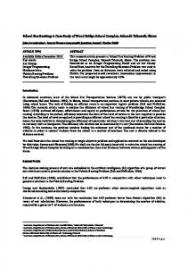
which is forwarded by a node to another node whose x coordinate is smaller by 1 until anchor X is reached. Each node that receives the Equator SET message is on the equator and generates the Meridian+ SET and Meridian- SET messages. The Meridian+ SET (or Meridian- SET) message is forwarded by a node to another node whose z (or z ′ ) coordinate is smaller by 1 until anchor Z (or Z ′ ) is reached. Each node that receives the Meridian+ SET or Meridian- SET message generated by the node whose x coordinate equals i is on the i-th meridian. For a node, U , on the i-th meridian, the ripple and longitude coordinates are assigned to 0 and i, respectively. The latitude coordinate of U is assigned to the hop distance from the equator on the i-th meridian if U is on the shortest path from a node on the equator to anchor Z; otherwise, the latitude coordinate is assigned to the negative value of the hop distance from the equator on the i-th meridian. If U is located on k meridians, U is assigned k longitude, latitude, and ripple coordinates, as implemented in the following. Once a node receives the Equator SET message, the node assigns the longitude and latitude coordinates to its x coordinate and 0, respectively. A Meridian+ SET (or Meridian- SET) message contains the x and z (or z ′ ) coordinates of the node that generates the message. Once a node receives the Meridian+ SET (or Meridian- SET) message generated by node U , the node assigns the longitude coordinate to the x coordinate of U , and the latitude coordinate to the z coordinate of U minus its z coordinate (or its z ′ coordinate minus the z ′ coordinate of U ). The node whose longitude coordinate equals i on the equator is the longitude head LH(i). The node whose latitude coordinate equals j on the i-th meridian is the cell head CH(i, j). Algorithm 2 describes how to establish axes and assign the longitude, latitude, and ripple coordinates for axis nodes. Fig. 2 illustrates a snapshot of the establishment of axes in the network consisting of around 2000 nodes. A.3 Assignment of Longitude, Latitude, and Ripple Coordinates A new phase initiates after all axis nodes have been assigned the longitude, latitude, and ripple coordinates. The longitude

X

Z

Z'

Y

Fig. 2. A snapshot of the establishment of axes in ABVCap.

and latitude coordinates of each non-axis node are assigned to the longitude and latitude coordinates of the cell head from which the node has the minimum hop distance. The ripple coordinate of each non-axis node is assigned to the minimum hop distance from the cell head, as implemented in the following. Every axis node generates a 3COOR SET message which is broadcast in a manner analogous to that for the X SET message. The 3COOR SET message contains the longitude and latitude coordinates of the node, U , that generates the message and a hop counter initially set to 1 and advanced in increments by the forwarding nodes. A nonaxis node assigns the longitude and latitude coordinates to the longitude and latitude coordinates of U , and assigns the ripple coordinate to the hop counter according to the 3COOR SET message with the smallest hop counter. Algorithm 3 describes how a non-axis node assigns the longitude, latitude, and ripple coordinates.

A.4 Assignment of Up and Down Coordinates After the longitude, latitude, and ripple coordinates have been designated for all nodes, the next phase involves the assignment of the up and down coordinates. Each virtual node in the longitude region of anchor Y (or X) assigns the up (or down) coordinate to 0. It is noted that each virtual node knows the longitude coordinate of anchor Y in the election of anchor Y . Each other virtual node, u, in N ET (i) assigns the up (or down) coordinate to the number of internal nodes on the shortest path, passing through the virtual nodes in N ET (i), from u to a virtual node in N ET (i + 1) (or N ET (i − 1)), as implemented in the following. Every virtual node that has one neighbor whose longitude coordinate is larger (or smaller) by 1 assigns the up (or down) coordinate to 0 and generates an UP SET (or DOWN SET) message containing its longitude coordinate and a hop counter initially set to 1 and advanced in increments by the forwarding nodes. The UP SET (or DOWN SET) message is broadcast between virtual nodes in a longitude region in a manner analogous to that for the X SET message between nodes in the whole network. The other virtual node assigns the up (or down) coordinate to the smallest hop counter contained in the UP SET (or DOWN SET) message received. Algorithm 4 describes how a virtual node assigns the up coordinate.

5

Algorithm 3 1. For any axis node: a) Generate and broadcast a 3COOR SET message containing its longitude and latitude coordinates and a hop counter set to 1. 2. For any non-axis node receiving a 3COOR SET message: a) Assign the longitude and latitude coordinates to the longitude and latitude coordinates of the node that generates the message, assign the ripple coordinate to the hop counter contained in the message, and broadcast the message, if the message contains the smallest hop counter among all 3COOR SET messages received. Algorithm 4 1. For any virtual node in the longitude region of anchor Y : a) Assign the up coordinate to 0. 2. For any virtual node having one neighbor whose longitude coordinate is larger by 1: a) Generate and broadcast an UP SET message containing its longitude coordinate and a hop counter set to 1, and assign the up coordinate to 0. 3. For any other virtual node receiving a UP SET message: a) Assign the up coordinate to the hop counter contained in the message, and broadcast the message with the hop counter increased by 1, if the message is generated by a virtual node in the same longitude region and contains the smallest hop counter among all UP SET messages received.

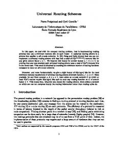
B. An ABVCap Example An example of the assignment of the virtual coordinates using ABVCap is presented in Fig. 3. In the first phase, node 22 is sink W . Nodes 25, 24, 23, 22 are selected as anchors X, Y , Z, and Z ′ , respectively. In the second phase, the longitude, latitude, and ripple coordinates of node 6 are assigned to 2, 0, and 0, respectively, because node 6 whose x coordinate equals 2 receives the Equator SET message. The longitude, latitude, and ripple coordinates of node 3 are assigned to 2, -1, and 0, respectively, because node 3 whose z ′ coordinate equals 1 receives the Meridian- SET message generated by node 6 whose x and z ′ coordinates equal 2. In the third phase, the longitude, latitude, and ripple coordinates of node 15 are assigned to 2, -1, and 1, respectively, because node 15 receives the 3COOR SET message with the minimum hop counter equal to 1 generated by node 3. In the fourth phase, the virtual node contained in node 3 assigns the up coordinate to 0 because it has a neighbor contained in node 2 whose longitude coordinate is larger by 1. The virtual node contained in node 15 assigns the up coordinate to 1 because it receives an UP SET message with the hop counter equal to 1 generated by the virtual node contained in node 3. Note that node 5 is assigned two virtual coordinates (0, −2, 0, 0, 0) and (1, −1, 0, 0, 0). Thus, node 5 contains two virtual nodes with virtual coordinates (0, −2, 0, 0, 0) and (1, −1, 0, 0, 0), respectively. C. Correctness of ABVCap Only a connected network is considered here. Lemma 1 and Lemma 2 show that the subnetwork induced by the virtual nodes in a cell region and in a longitude region in ABVCap

(3, 1, 0, 0, 0) (4, 1, 0, 0, 0) 2

(0, 3, 0, 0, 0) (3, 2, 0, 0, 0) (1, 2, 0, 0, 0) (4, 2, 0, 0, 0) 22 (2, 2, 0, 0, 0) 21 (4, 0,1, 0, 0) 20 (0, 2,1, 0, 0) (2, 1, 0, 0, 0) (3,1, 0, 0, 0) (1, 1,1, 0, 0)  (2, 1,1,1,1) 3 (4,1, 0, 0, 0) 1 15 (0, 2, 0, 0, 0) 11 (3, 0, 0, 0, 0) 5 (1, 1, 0, 0, 0) 16 4 17 (3, 0,1,1, 0) 12 (2, 0,1, 0, 0) (2, 0,1, 0,1) 6 13 (0, 0,1, 0, 0) (2, 0, 0, 0, 0) 18 Z 23 8 14 (0, 1, 0, 0, 0) (0,3, 0, 0, 0) (0, 2,1, 0, 0) (1, 0,1, 0, 0) (1, 0, 0, 0, 0) 25 X (1, 2, 0, 0, 0) (1,1,1, 0, 0) 7 (0, 0, 0, 0, 0) 10 (2,1, 0, 0, 0) 19 (0, 2, 0, 0, 0) (1, 0,1,1, 0) (3, 2, 0, 0, 0) (0,1,1, 0, 0) (1,1, 0, 0, 0) (4, 2, 0, 0, 0) (0,1, 0, 0, 0) 9

(4, 0, 0, 0, 0) Y 24

Z'

Fig. 3. Example of ABVCap. The number inside the circle denotes the node ID. The 1st , 2nd , 3rd , 4th , and 5th entries in the parentheses denote the longitude, latitude, ripple, up, and down coordinates, respectively.

is connected, respectively. Theorem 1 shows that ABVCap assigns at least one 5-tuple virtual coordinate to each node. Lemma 1: In ABVCap, the virtual nodes in a cell region induce a connected subnetwork. Proof: It suffices to show there exists a path in N ET (i1 , j1 ) between u and CH(i1 , j1 ) for each virtual node, u, in cell region (i1 , j1 ). Suppose that u assigns its longitude, latitude, and ripple coordinates when it receives the 3COOR SET message m1 generated by CH(i1 , j1 ). Let P (P = v1 , v2 , ..., vk ) be the path traversed by message m1 from v1 = CH(i1 , j1 ) to vk = u. We show all virtual nodes v1 , v2 , ..., vk are in cell region (i1 , j1 ). Suppose a virtual node exists, say vi (1 < i < k), that is not in cell region (i1 , j1 ). This implies that vi receives the 3COOR SET message m2 generated by CH(i2 , j2 ) (i1 6= i2 or j1 6= j2 ) after vi receives the 3COOR SET message m1 and the hop counter contained in message m2 is less than the one contained in message m1 . In this case, u must update the longitude and latitude coordinates to i2 and j2 , respectively, after u receives the 3COOR SET message m2 . This implies that u is in cell region (i2 , j2 ), constituting a contradiction. Lemma 2: In ABVCap, the virtual nodes in a longitude region induce a connected subnetwork. Proof: Let u and v be two virtual nodes in longitude region i. Suppose that u and v are in cell regions (i, j1 ) and (i, j2 ), respectively. According to Lemma 1, there is a path in N ET (i, j1 ) between u and CH(i, j1 ), and there is a path in N ET (i, j2 ) between v and CH(i, j2 ). Because there exists a path in N ET (i) between CH(i, j1 ) and CH(i, j2 ), there exists a path in N ET (i) between u and v. Theorem 1: ABVCap assigns each node at least one 5-tuple virtual coordinate. Proof: First note that ABVCap assigns each node at least one longitude, one latitude, and one ripple coordinates since the network is connected. We need to show that each virtual node u with the 3-tuple virtual coordinate (u.lo, u.la, u.rp) must be assigned u.up and u.dn. The proof of assigning u.up is omitted due to its similarity with that of assigning u.dn. Consider a virtual node u. If u.lo = 0, u.dn is assigned to

6

0; otherwise, u.dn is assigned after u receives a DOWN SET message or generates a DOWN SET message. It suffices to show u receives at least one DOWN SET message if u does not generate a DOWN SET message. Let u be in longitude region i. The virtual node LH(i) must generate a DOWN SET message because LH(i) has a neighbor LH(i − 1). Because there is a path from LH(i) to u in N ET (i) according to Lemma 2, u receives the DOWN SET message generated by LH(i) if u receives no other DOWN SET message. IV. ABVC AP ROUTING We assume that a node receives all multiple virtual coordinates of all neighbors. We also assume that the virtual coordinate of the destination received by the source is unique [14], [20]. In ABVCap routing, the routed packet contains the longitude and latitude coordinates of the destination. ABVCap routing is described in subsection A. An ABVCap routing example is given in subsection B. And, we show ABVCap routing can always route the packet from the source to the destination in subsection C. The following notations are necessary for the description of ABVCap routing. Definition 3: The pair of numbers a and b is defined to be smaller than the pair of numbers c and d, denoted by (a, b) < (c, d), if a < c, or a = c and b < d. Definition 4: Given two virtual nodes u and v, the longitude distance is defined to be |u.lo − v.lo|, and the latitude distance is defined to be |u.la − v.la|. Definition 5: Given destination d, for virtual node u, the notation u.rep denotes u.up if u.lo < d.lo, denotes u.dn if u.lo > d.lo, and denotes |u.la − d.la| if u.lo = d.lo. A. The Routing Protocol A packet in N ET (i) can reach N ET (i + 1) (or N ET (i − 1)) if the packet is repeatedly forwarded to a neighbor having a smaller up (or down) coordinate. This implies that a packet always can be routed to a virtual node in the longitude region of the destination. A packet in N ET (i, j) can reach N ET (i, j + 1) (or N ET (i, j − 1)) if the packet is first routed to CH(i, j) by being repeatedly forwarded to a neighbor having a smaller ripple coordinate, and subsequently routed to CH(i, j + 1) (or CH(i, j − 1)) via the link between CH(i, j) and CH(i, j +1) (or CH(i, j −1)). Therefore, a packet always can be routed to a virtual node in the cell region of the destination. Proactive routing can eventually route the packet to the destination because the virtual nodes in the cell region of the destination induce a connected subnetwork. ABVCap routing forwards the packet using the greedy method. The packet is first routed to a virtual node in the longitude region of the destination (longitude routing), then to a virtual node in the cell region of the destination (latitude routing), and finally to the destination using proactive routing. If a node, U , contains no virtual node in the longitude region of the destination, U routes a packet using longitude routing; otherwise, if U contains no virtual node in the cell region of the destination, U routes a packet using latitude routing. Otherwise, U routes a packet using proactive routing. In longitude routing, U forwards the packet to the virtual node with the minimum

Algorithm 5 1. For any node, U , that contains no virtual node in the longitude region of the destination (longitude routing): a) U forwards the packet to the virtual node, v, with the smallest pair of numbers (|v.lo − d.lo|, v.rep) among all virtual nodes contained in the neighbors of U . 2. For any other node, U , that contains no virtual node in the cell region of the destination (latitude routing): a) U forwards the packet to the virtual node, v, with the smallest pair of numbers (|v.la − d.la|, v.rp) among all virtual nodes contained in the neighbors of U in the longitude region of the destination. 3. For any other node, U (proactive routing): a) U forwards the packet to the next hop in the local routing table.

longitude distance from the destination among all virtual nodes contained in the neighbors of U , or, in case of a tie, the virtual node, v, with the smallest number v.rep. In latitude routing, U forwards the packet to the virtual node with the same longitude coordinate as the destination and the minimum latitude distance from the destination among all virtual nodes contained in the neighbors of U , or, in case of a tie, the virtual node with the smallest ripple coordinate. In proactive routing, each node constructs a local routing table that contains routing information for virtual nodes in the same cell region. Algorithm 5 describes how a node routes a packet using ABVCap routing in a network. B. An ABVCap Routing Example Consider the packet routed by ABVCap routing from node 18 to node 15 in Fig. 3. Firstly, Node 18 proceeds with longitude routing because it contains no virtual node in the longitude region of the destination. The packet is forwarded to node 6 because node 6 contains the virtual node, v, that has the smallest pair of numbers (|v.lo − d.lo|, v.rep), equal to (0, 1), among all virtual nodes contained in the neighbors of node 18. Then, node 6 proceeds with latitude routing because it contains a virtual node in the longitude region of the destination. The packet is forwarded to node 3 because node 3 contains the virtual node, v, that has the smallest pair of numbers (|v.la−d.la|, v.rp), equal to (0, 0), among all virtual nodes contained in the neighbors of node 6 in the longitude region of the destination. Finally, node 3 routes the packet to node 15 using proactive routing because node 3 contains a virtual node in the cell region of the destination. C. Guaranteed Delivery of ABVCap Routing Theorem 2 shows that ABVCap routing guarantees packet delivery, where packet loss and other realistic failures are not considered. Theorem 2: ABVCap routing always routes the packet from the source, s, to the destination, d. Proof: We first show longitude routing can forward the packet to a virtual node, v, with v.lo = d.lo. Let ui be the i-th forwarding virtual node. It suffices to show claim 1: (|ui+1 .lo − d.lo|, ui+1 .rep) < (|ui .lo − d.lo|, ui .rep) for all i. Because ui+1 has the smallest pair of numbers (|v.lo − d.lo|, v.rep) among all neighbors, v, of ui , we

7

TABLE I. Summary of Methods in ABVCap and ABVCap Maintenance Methods Maximum Hops Shortest Path Clustering Relaxation Message Pruning Primary Backup

Applied Places Election of Anchors Establishment of Axes, Reconstruction of Axes Assignment of Longitude, Latitude, and Ripple Coordinates Assignment of Up and Down Coordinates, Update of Ripple, Up, and Down Coordinates Election of Anchors, Assignment of Longitude, Latitude, and Ripple Coordinates, Assignment of Up and Down Coordinates, Election of New Anchors Election of New Anchors

only need to show that ui has a neighbor, v, such that (|v.lo− d.lo|, v.rep) < (|ui .lo− d.lo|, ui .rep). Without loss of generality, we assume that ui .lo < d.lo. If ui .up = 0, ui has a neighbor, v, with v.lo = ui .lo + 1, and if ui .up 6= 0, ui has a neighbor, v, with v.lo = ui .lo and v.up = ui .up − 1, in which cases (|v.lo − d.lo|, v.rep) < (|ui .lo − d.lo|, ui .rep). Next, we show latitude routing can forward the packet to a virtual node, v, with v.lo = d.lo and v.la = d.la. Let ui be the i-th forwarding virtual node in latitude routing. It suffices to show claim 2: ui+1 .lo = ui .lo and (|ui+1 .la − d.la|, ui+1 .rp) < (|ui .la− d.la|, ui .rp) for all i. The proof of claim 2 is omitted due to its similarity with that of claim 1. Because the virtual nodes in a cell region induce a connected subnetwork by Lemma 1, the packet can always be routed to the destination using proactive routing.

Algorithm 6 1. For any backup node detecting the failure of anchor X: a) Generate an X RESET message containing its ID (the source ID) and the IDs of its chosen backup nodes. b) Create a virtual node with the virtual coordinate (0, 0, 0, ∞, ∞), if its ID is larger than any other source ID contained in the X RESET message received. 2. For any node: a) Broadcast the X RESET message generated or received, if the message contains the maximum source ID among all X RESET messages generated or received.

elected, it selects a certain number of nodes from the neighbors as its backup nodes. As the backup node detects the failure of X, the node generates an X RESET message containing its ID (the source ID) and the IDs of its chosen backup nodes. Once a node generates or receives an X RESET message, the node broadcasts the message containing the maximum source ID. A backup node is new anchor X if its ID is larger than any other source ID contained in the X RESET message received. New anchor X creates a new virtual node with the longitude, latitude, and ripple coordinates equal to 0 to become the new longitude head LH(0) and the new cell head CH(0, 0). The up and down coordinates of the new virtual node are initially set to ∞. Algorithm 6 describes how new anchor X is elected. New anchors Y , Z, and Z ′ are elected in a manner analogous to that for election of new anchor X.

V. ABVC AP M AINTENANCE ABVCap maintenance is described in subsection A. An ABVCap maintenance example is given in subsection B. And, in subsection C, we show that ABVCap routing can always route the packet from the source to the destination in a network with node failures. Table I summarizes the methods used in ABVCap and ABVCap Maintenance. A. The Maintenance Protocol To guarantee packet delivery, each subnetwork, N ET (i), and each subnetwork, N ET (i, j), must be connected. Each virtual node, which is not in the longitude region of anchor Y (or X), must have a neighbor with a smaller up (or down) coordinate in the same longitude region if the node has no neighbor in the longitude region larger (or smaller) by 1. Each virtual node must have a neighbor with a smaller ripple coordinate in the same cell region if the node is not a cell head. To this purpose, ABVCap maintenance keeps each anchor alive using the primary backup approach, as described in subsection A.1, and connects any two disconnected sub-axes using the shortest path method, as described in subsection A.2. Also, the ripple, up, and down coordinates of the virtual nodes are updated using the node relaxation technique, as described in subsection A.3. In subsection A.4, ABVCap routing in a network with node failures is presented. A.1 Election of New Anchors When an anchor fails, the node with the maximum ID among all the backup nodes of the anchor is elected as the new anchor, as implemented in the following. Once anchor X is

A.2 Reconstruction of Axes When longitude heads LH(j +1), LH(j +2), ..., LH(k−1) fail on the equator, the shortest path between LH(j) and LH(k) is established in a manner analogous to that for the shortest path between anchors X and Y (the equator), as implemented in the following. Once LH(j) detects that LH(j +1) is not in the 1-hop neighborhood, LH(j) generates an Equator REP message containing the longitude coordinate of LH(j) and a hop counter initially set to 1 and advanced in increments by the forwarding nodes. Once a node receives the Equator REP message generated by LH(j), the node stores the hop counter contained in the message (the hop distance from LH(j)) and broadcasts the message if the message contains the smallest hop counter. After LH(k) detects LH(k − 1) is not in the 1-hop neighborhood and receives the Equator REP message generated by LH(j), it generates an Equator RESET message containing the longitude coordinate of LH(j), which is forwarded by a node to another node whose hop distance from LH(j) is smaller by 1 until LH(j) is reached. If LH(k) receives the Equator REP messages generated by more than one longitude head because the equator is separated into more than two sub-axes, it establishes the shortest path to the longitude head that has the smallest longitude distance from LH(k) among all longitude heads generating the Equator REP messages and having a smaller longitude coordinate than LH(k). In addition, if new anchor X is not in the 1-hop neighborhood of LH(1), the shortest path is established between new anchor X and LH(1). Once the shortest path between LH(j) and LH(k) is established, nodes on the path create virtual nodes that are

8

Algorithm 7 1. For any EQ(j) detecting EQ(j + 1) is not in the 1-hop neighborhood: a) Generate an Equator REP message containing the longitude coordinate of EQ(j) and a hop counter set to 1. 2. For any node receiving an Equator REP message generated by EQ(j): a) Store the hop counter contained in the message, and broadcast the message with the hop counter increased by 1, if the message contains the smallest hop counter among all received Equator SET messages generated by EQ(j). 3. For any EQ(k) detecting EQ(k − 1) is not in the 1hop neighborhood and receiving the Equator REP message generated by EQ(j), where EQ(j) has a smaller longitude distance from EQ(k) than any other virtual node that has a smaller longitude coordinate than EQ(k) and generates an Equator REP message: a) Reset the longitude distance per hop to 1 and the node containing EQ(k) creates i virtual nodes, which have longitude coordinates equal to EQ(k).lo−i, · · · , EQ(k).lo− 1, the latitude and ripple coordinates equal to 0, and the up and down coordinates equal to ∞, to be longitude heads LH(⌊EQ(k).lo⌋ − i), · · · , LH(⌊EQ(k).lo⌋ − 1), if the longitude distance per hop is larger than 1, where i equals the absolute difference, in terms of the integer part of the longitude coordinate, between EQ(j) and EQ(k) minus the hop distance between EQ(j) and EQ(k). b) Generate an Equator RESET message containing the longitude coordinate of EQ(j) and the longitude distance per hop. 4. For any node receiving an Equator RESET message containing the longitude coordinate of EQ(j): a) Forward the Equator RESET message to a neighbor with a smaller hop distance from EQ(j). b) Create a virtual node, u, with the longitude coordinate equal to the longitude coordinate of EQ(j) plus the multiplication of the longitude distance per hop and the hop distance from EQ(j), the latitude coordinate equal to 0, and the ripple, up, and down coordinates equal to ∞. c) Reset the ripple coordinate of u to 0, if the difference between the longitude coordinate of u and the longitude distance per hop is less than the integer part of the longitude coordinate of u.

assigned the longitude coordinates in an increasing order, as implemented in the following. The Equator RESET message generated by LH(k) contains the ratio of the longitude distance between LH(j) and LH(k) to the hop distance between LH(j) and LH(k) (the longitude distance per hop). Each node that receives the Equator RESET message creates a new virtual node with the latitude coordinate equal to 0 and the longitude coordinate equal to the longitude coordinate of LH(j) plus the multiplication of the longitude distance per hop and the hop distance from LH(j). The ripple, up, and down coordinates of the new virtual nodes are initially set to ∞. Note that if the longitude distance per hop is larger than 1, a longitude head is not assigned to every longitude region. In this case, the longitude distance per hop contained in the Equator RESET message is set to 1, and LH(k) creates i virtual nodes to be longitude heads LH(k−i), · · · , LH(k−1), where i denotes the longitude distance between LH(j) and LH(k) minus the hop distance between LH(j) and LH(k). After the reconstruction of the equator, the longitude coordinate of a virtual node on the equator could be a non-integer.

In this paper, the virtual node with the longitude coordinate equal to i is said to be in longitude region ⌊i⌋. A virtual node on the equator is the longitude head LH(i) and the cell head CH(i, 0), if it has the smallest longitude coordinate among all virtual nodes on the equator in longitude region i. A virtual node resets the ripple coordinate to 0 if it is a longitude head. Algorithm 7 describes the reconstruction of the equator that consists of virtual nodes EQ(0), · · · , EQ(m), where EQ(0) and EQ(m) are contained in anchors X and Y , respectively, and EQ(i) denotes the virtual node on the equator with the hop distance from X equal to i (EQ(i) may not be a longitude head and may have a non-integer longitude coordinate). In Algorithm 7, virtual node u detects the disappearance of virtual node v, if the node containing u detects the disappearance of the node containing v. Furthermore, if LH(i) fails, a new LH(i) is first generated in the reconstruction of the equator. Subsequently, each of the i-th meridians from LH(i) to anchor Z and the i-th meridian from LH(i) to anchor Z ′ are reconstructed in a manner analogous to that for the reconstruction of the equator from anchor X to anchor Y . Each virtual node with the latitude coordinate equal to j on the i-th meridian is the cell head CH(i, j), where j could be a non-integer. The ripple coordinate of each cell head is set to 0, and the up and down coordinates are initially set to ∞. A.3 Update of Ripple, Up, and Down Coordinates If a virtual node that is not a cell head has no neighbor with a smaller ripple coordinate in the same cell region, it updates the ripple coordinate to ∞. Once a virtual node updates the ripple coordinate, it broadcasts a RP CHANGE message containing its longitude, latitude, and updated ripple coordinates. A virtual node that is not a cell head checks if it has a neighbor with a smaller ripple coordinate in the same cell region as it detects the failure of any neighbor or receives a RP CHANGE message. For each period of time, the virtual node with the ripple coordinate equal to ∞ resets the ripple coordinate to one plus the smallest ripple coordinate of the neighbors, if exists, having the ripple coordinates not equal to ∞ in the same cell region. In addition, if a virtual node has the ripple coordinate equal to ∞ for t periods of time because the cell region of the virtual node is not connected, it resets the longitude and latitude coordinates to join another cell region. If a virtual node joins another cell region, it broadcasts a CELL CHANGE message containing its updated and original longitude, updated and original latitude, and updated ripple coordinates. Algorithm 8 describes how a virtual node updates the ripple coordinate. The up (or down) coordinate for a virtual node is updated in a manner analogous to that for the ripple coordinate. A.4 ABVCap Routing in a Network with Node Failures In a network with node failures, the longitude coordinate of a virtual node could be a non-integer. In this case, as mentioned before, the virtual node with the longitude coordinate equal to i is regarded to be in longitude region ⌊i⌋. In ABVCap routing, the virtual node with the longitude coordinate equal to

9

Algorithm 8 1. For any virtual node, which is not a cell head and has the ripple coordinate not equal to ∞, detecting the failure of any neighbor or receiving a RP CHANGE or CELL CHANGE message: a) Assign the ripple coordinate to ∞, if the virtual node has no neighbor with a smaller ripple coordinate in the same cell region. b) Broadcast a RP CHANGE message containing its longitude, latitude, and updated ripple coordinates, if the virtual node updates the ripple coordinate. 2. In each period of time, for any virtual node with the ripple coordinate equal to ∞: a) Assign the ripple coordinate to u.rp + 1, if the virtual node has a neighbor, u, with the smallest ripple coordinate not equal to ∞ in the same cell region. b) Broadcast a RP CHANGE message containing its longitude, latitude, and updated ripple coordinates, if the virtual node updates the ripple coordinate. 3. In each period of time, for any virtual node with the ripple coordinate equal to ∞ for t periods of time: a) Assign its longitude, latitude, and ripple coordinates to u.lo, u.la, u.rp + 1, respectively, if the virtual node has a neighbor, u, with the smallest ripple coordinate not equal to ∞ in a different cell region. b) Broadcast a CELL CHANGE message containing its updated and original longitude, updated and original latitude, and updated ripple coordinates, if the virtual node joins another cell region.

i is regarded as with the longitude coordinate equal to ⌊i⌋, as described in Algorithm 9. The following notation is necessary for the description of Algorithm 9. Definition 6: For virtual node u, the notation u.repm denotes u.up if ⌊u.lo⌋ < ⌊d.lo⌋, denotes u.dn if ⌊u.lo⌋ > ⌊d.lo⌋, and denotes |u.la − d.la| if ⌊u.lo⌋ = ⌊d.lo⌋, where d.lo and d.la denote the longitude and latitude coordinates of the destination. B. An ABVCap Maintenance Example An example of reconstructing the virtual coordinate system in the network shown in Fig. 3 with the failures of nodes 6 and 25 using ABVCap maintenance is presented in Fig. 4. As illustrated in Fig. 3, LH(0), LH(1), LH(2), and LH(3) are contained in nodes 25, 14, 6, and 1, respectively. Let nodes 12 and 19 be the backup nodes of anchor X (LH(0)). After the failures of nodes 6 and 25, node 19 becomes the new anchor X and creates a virtual node with the virtual coordinate (0, 0, 0, ∞, ∞) because node 19 has a larger ID than node 12. The new virtual node is the new longitude head LH(0) and the new cell head CH(0, 0). Subsequently, because LH(0) detects that LH(1) is not in the 1-hop neighborhood, LH(0) generates an Equator REP message. LH(1) also generates an Equator REP message because LH(1) detects that LH(2) is not in the 1-hop neighborhood. The Equator REP messages generated by LH(0) and LH(1) contain the longitude coordinates of LH(0) and LH(1), respectively. Once LH(3) receives the Equator REP messages generated by LH(0) and LH(1), LH(3) generates an Equator RESET message containing the longitude coordinate of LH(1) because LH(1) has a smaller longitude distance from LH(3) than LH(0). The Equator RESET message

Algorithm 9 1. For any node, U , that contains no virtual node in the longitude region of the destination (longitude routing): a) U forwards the packet to the virtual node, v, with the smallest pair of numbers (|⌊v.lo⌋ − ⌊d.lo⌋|, v.repm ) among all virtual nodes contained in the neighbors of U . 2. For any other node, U , that contains no virtual node in the cell region of the destination (latitude routing): a) U forwards the packet to the virtual node, v, with the smallest pair of numbers (|v.la − d.la|, v.rp) among all virtual nodes contained in the neighbors of U in the longitude region of the destination. 3. For any other node, U (proactive routing): a) U forwards the packet to the next hop in the local routing table.

also contains the longitude distance per hop, equal to the ratio of 2 (the longitude distance between LH(1) and LH(3)) to 3 (the hop distance between between LH(1) and LH(3)). The Equator RESET message is forwarded to node 16 that has a smaller hop distance from LH(1) than LH(3). Once node 16 receives the Equator RESET message, node 16 creates a virtual node with the virtual coordinate ( 73 , 0, ∞, ∞, ∞), where the longitude coordinate is assigned to 1 (the longitude coordinate of LH(1)) plus the multiplication of 23 (the longitude distance per hop) and 2 (the hop distance from LH(1)). The new virtual node is the new longitude head LH(2) and the new cell head CH(2, 0) because the neighbor with a smaller longitude coordinate on the equator has the longitude coordinate equal to 73 − 23 and is in longitude region 1. Similarly, node 16 forwards the Equator RESET message to node 4, and node 4 creates a virtual node with the virtual coordinate ( 53 , 0, ∞, ∞, ∞). Node 4 forwards the Equator RESET message to node 14, which contains LH(1). Thereby, the reconstruction of the equator between LH(1) and LH(3) is completed. Similarly, once LH(1) receives the Equator REP message generated by LH(0), LH(1) generates an Equator RESET message to reconstruct the equator between LH(0) and LH(1). Additionally, because the new cell head CH(2, 0) (contained in node 16) is disconnected from CH(2, 1) (contained in node 23), the meridian from CH(2, 0) to CH(2, 1) is reconstructed in a manner similar to that for the reconstruction of the equator from LH(0) (anchor X) to LH(1). Moreover, if node 12 detects the failure of node 25, the virtual node contained in node 12 assigns the ripple coordinate to ∞ because it has no neighbor with a smaller ripple coordinate in cell region (0, 0). After t periods of time, the virtual node contained in node 12 joins cell region (0, −1) and assigns the ripple coordinate to be equal to 1 because it has a neighbor with the ripple coordinate equal to 0 (contained in node 13) in cell region (0, −1). C. Correctness of ABVCap Maintenance We assume that the network is connected after node failures. We also assume that an anchor and its backup nodes do not fail simultaneously. Theorem 3 shows that ABVCap routing guarantees packet delivery in a network with node failures. Lemma 3 is used to prove Theorem 3.

10

(3, 1, 0, 0, 0) (4, 1, 0, 0, 0) 2

(0, 3, 0, 0, 0) (3, 2, 0, 0, 0) (1, 2, 0, 0, 0) (4, 2, 0, 0, 0) 22 (2, 2, 0, 0, 0) 21 (4, 0,1, 0, 0) (0, 2,1, 0, 0) 20 (2, 1, 0, 0, 0) (3,1, 0, 0, 0) (1, 1,1, 0, 0) 3 (2, 1,1,1,1) (4,1, 0, 0, 0) 1 15 (0, 2, 0, 0, 0) 11 (3, 0, 0, 0, 0) 5 (1, 1, 0, 0, 0) 16 4 17 (3, 0,1,1, 0) 12 (7 3, 0, 0, 0, 0) (2, 0,1, 0, 0) (2, 0,1, 0,1) 6 (5 3, 0,1, 0, 0) 13 (0, 1,1, 0, 0) 18 Z 23 8 14 (0, 1, 0, 0, 0) (0,3, 0, 0, 0) (0, 2,1, 0, 0) (1, 0,1, 0, 0) (1, 0, 0, 0, 0) (2,1 3, 0, 0, 0) 25 (1, 2, 0, 0, 0) (1,1,1, 0, 0) (2, 2 3, 0, 0, 0) 7 10 (2,1, 0, 0, 0) 19 X (0, 2, 0, 0, 0) (1, 0,1,1, 0) (3, 2, 0, 0, 0) (1 2, 0,1, 0, 0) (0,1,1, 0, 0) (1,1, 0, 0, 0) (4, 2, 0, 0, 0) (0, 0, 0, 0, 0) (0,1, 0, 0, 0) 9

(4, 0, 0, 0, 0) Y 24

Z'

Fig. 4. Example of ABVCap maintenance.

Lemma 3: ABVCap maintenance assigns each virtual node ripple, up, and down coordinates smaller than ∞. Proof: The proofs for the up and down coordinates are omitted due to their similarities to that for the ripple coordinate. After t periods of time, a virtual node has the ripple coordinate equal to ∞ only if each neighbor has the ripple coordinate equal to ∞. Therefore, after t periods of time, if a virtual node with the ripple coordinate equal to ∞ exists, the ripple coordinate of each virtual node equals ∞ by repeating the same argument, which is impossible because the ripple coordinate of each cell head equals 0. Theorem 3: ABVCap routing always routes the packet from the source to the destination. Proof: In ABVCap maintenance, a virtual node has the ripple coordinate between 0 and ∞ only if the virtual node has a neighbor with a smaller ripple coordinate in the same cell region, and has the up (or down) coordinate between 0 and ∞ only if the virtual node has a neighbor with a smaller up (or down) coordinate in the same longitude region. Lemma 3 implies that longitude routing always forwards the packet to a virtual node in the longitude region of the destination, and latitude routing always forwards the packet to a virtual node in the cell region of the destination using the same argument in the proof of Theorem 2. We need to show that virtual nodes in a cell region induce a connected subnetwork so that proactive routing always forwards the packet to the destination. It suffices to show there exists a path in N ET (i1 , j1 ) between u and CH(i1 , j1 ) for each virtual node, u, in cell region (i1 , j1 ). Let P = v1 , v2 , ..., vk be the longest path in N ET (i1 , j1 ) from u such that the virtual nodes on the path have ripple coordinates in a decreasing order. We show vk = CH(i1 , j1 ). If vk 6= CH(i1 , j1 ), vk has a neighbor, vk+1 , in cell region (i1 , j1 ) with a smaller ripple coordinate. Then, P ′ = v1 , v2 , ..., vk , vk+1 is a longer path than P , constituting a contradiction. VI. A NALYSIS

OF

M ESSAGE OVERHEAD PATH L ENGTH

AND

ROUTING

We first study the message overhead of ABVCap and ABVCap maintenance by examining the number of messages

required to be broadcast. Subsequently, we analyze the route stretch of ABVCap routing. A. Message Overhead In ABVCap, in the first phase, sink W first generates a W SET message to assign the w coordinate to each node. Each node also obtains the w coordinate of each neighbor from the W SET messages received. This requires approximately one message broadcast by each node if each packet travels at approximately the same speed. Subsequently, every node broadcasts the ID and the w coordinate of the node with the maximum w coordinate in the 1-hop neighborhood, or, in case of a tie, the node with the maximum ID. This requires one message to be broadcast by each node. Then, every node with the maximum w coordinate in the 2-hop neighborhood, or, in case of a tie, the node with the maximum ID, broadcasts an X SET message to assign the x coordinate to each node. In [4], a well-known technique on trading time for communication is used so that only one X SET message is required to be broadcast by each node. Therefore, each node broadcasts two messages to assign the x coordinate. The y, z, and z ′ coordinate assignment is analogous to the x coordinate assignment. Thus, each node broadcasts approximately nine messages during this phase. In the second phase, Y is required to send a message to anchor X, and each node on the equator is required to send a message to anchors Z and Z ′ . In the third phase, each node must broadcast at least one 3COOR SET message. Each node broadcasts the 3COOR SET message approximately once if the axis nodes broadcast the 3COOR SET messages at approximately the same time [10], [24], and each packet travels at approximately the same speed. This requires approximately one message broadcast by each node. In the fourth phase, each virtual node, u, must broadcast at least one UP SET (or DOWN SET) message if the virtual node is not in the longitude region of anchor Y (or X). Each virtual node broadcasts the UP SET (or DOWN SET) message approximately once if the UP SET (or DOWN SET) messages in a longitude region are broadcast at approximately the same time, and each packet travels at approximately the same speed. Let k denote the average number of virtual coordinates per node. Then, each node broadcasts approximately 2k UP SET and DOWN SET messages during this phase. In ABVCap Maintenance, when an anchor fails, each backup node must generate one message to be broadcast in the network. This requires approximately one message broadcast by each node if the technique on trading time for communication is used. In the reconstruction of axes, one message must be generated and broadcast by each node to establish the shortest path between two disconnected sub-axes. B. Expected Routing Path Length Theorem 4 shows the route stretch of ABVCap routing in a boundless 2D space in a continuous domain, where nodes are assumed to be infinitely dense in a boundless 2D space. Theorem 4: Given the source s and the destination d, the expected ratio of the ABVCap routing path length to the shortest path length is π4 in a boundless 2D space in a continuous domain.

11

d r

T s

i

Fig. 5. Locations of the source s, the intermediate node i, and the destination d.

Proof: Assume that s and d are located on (0, 0) and (r cos θ, r sin θ), respectively. Using ABVCap routing, the packet is first routed to an intermediate node i, located on (r cos θ, 0), in longitude routing, and then routed to d in latitude routing, as shown in Fig. 5. Since the probability 1 density function of θ is 2π , the expected ratio of the ABVCap routing path length to the shortest path length equals R 2π |r cos θ|+|r sin θ| 1 4 ( )( )dθ = r 2π π. 0 VII. P ERFORMANCE E VALUATION Simulations using the packet level simulator and the network simulator ns-2 (version 2.31) were used to evaluate the performance of the proposed protocols in networks with largescale size and network behaviors, respectively. The connected networks with density ranging from 10 to 30 were generated by randomly deploying nodes in square regions, where the network density denotes the average number of neighbors per node and the transmission range of nodes is a circle of radius 1. We compared ABVCap routing with GLIDER, Hop ID, GLDR, and VCap routing. In GLIDER, 23 landmarks were randomly selected. In Hop ID, the peripheral landmark selection of 30 landmarks and landmark-guided routing with t = 5 was implemented, where t is the maximum hops of allowed landmark-guided routing. In GLDR, 2-sampling and 10-sampling were used in square regions with side lengths equal to 10 and 50, respectively. The local detour rule with c = 2 was implemented in VCap, where c denotes the maximum number of allowed local detours per packet. The flooding mechanism used to route a packet to the destination when the packet encounters a dead-end node was not implemented in GLIDER, Hop ID, GLDR, or VCap routing because it required a great deal of route overhead and suffered from the broadcasting storm problem [25]. A. Simulation Results on a Packet Level Simulator In the simulation, 100 connected networks were generated in square regions with side lengths equal to 10 or 50. Each square region has 0 or 10 voids, in which the voids, denoting regions without nodes, were circles of radius 4 and could be overlapped. We investigated the average routing path length, the average packet delivery rate, the average number of next hop neighbors, and the load imbalance factor of GLIDER, Hop ID, GLDR, VCap, and ABVCap routing, in which the load imbalance factor denoted the ratio of the maximum number of packets routed by a node (the maximum load) to the average number of packets routed by a node (the average

load). The existence of a node that routes many packets was indicated by a large load imbalance factor. Empirical data were obtained by averaging data of 500 source-destination pairs from 100 networks. We also studied the average number of virtual coordinates assigned to each node by ABVCap in which empirical data were obtained by averaging data from 100 networks. A.1 Packet Delivery Rate Fig. 6 illustrates that ABVCap routing successfully sets a path for every source-destination pair. In GLIDER, Hop ID, GLDR, and VCap routing, the higher the network density, the higher the packet delivery rate because more dead-end nodes exist in a network with lower density due to the occurrence of more holes. As 10 voids were deployed, the packet delivery rate becomes lower because a packet has a higher probability to encounter dead-end nodes surrounding voids. In a smallscale network, the packet delivery rate is high due to the small average distance of source-destination pairs. Compared to Hop ID or GLDR routing, GLIDER and VCap routing each have a lower packet delivery rate resulting from the introduction of more dead-end nodes because large cells exist in GLIDER and multiple nodes share a virtual coordinate in VCap. A.2 Routing Path Length Fig. 7 demonstrates that ABVCap routing has a longer routing path than GLIDER, Hop ID, GLDR, and VCap routing. Two reasons exist to explain this observation: 1) ABVCap routing routes the packet similarly to using the L1 norm while GLIDER, Hop ID, GLDR, and VCap routing route the packet similarly to using the L2 norm, and 2) ABVCap routing has a longer average distance of source-destination pairs because many source-destination pairs separated by long distances are unreachable in GLIDER, Hop ID, GLDR, and VCap routing. In addition, the higher the network density, the shorter the routing path because the progress distance is larger. For a source-destination pair, the more voids exist, the longer the routing path will be because the longer path is set to bypass voids. In a small-scale network, the short routing path results from the small average distance of source-destination pairs. A.3 Number of Next Hop Neighbors Fig. 8(a) illustrates that a node has few next hop neighbors in Hop ID or VCap routing because it can only forward a packet to the neighbor having the smallest distance from the destination. In Hop ID routing, most nodes have only one next hop neighbor because a node is addressed by the hop distances from 30 landmarks. In Vcap, many nodes share a virtual coordinate because a node is addressed by the hop distances from 3 anchors. Thus, in Vcap routing, a node has more next hop neighbors compared to Hop ID routing. In GLIDER or GLDR routing, a node has many next hop neighbors because it can forward a packet to any neighbor having a smaller hop distance from the selected landmark. In GLIDER, GLDR, VCap, and ABVCap routing, the higher the network density, the more the next hop neighbors. A.4 Load Imbalance Factor

12

80

60 GLIDER Hop ID GLDR VCap ABVCap

40

100

Packet Delivery Rate (%)

100

Packet Delivery Rate (%)

Packet Delivery Rate (%)

100

80

60 GLIDER Hop ID GLDR VCap ABVCap

40 10

15

20 Network Density

25

30

80

60 GLIDER Hop ID GLDR VCap ABVCap

40 10

15

(a)

20 Network Density

25

30

10

15

(b)

20 Network Density

25

30

(c)

Fig. 6. Packet delivery rate of GLIDER, Hop ID, GLDR, VCap, and ABVCap routing on the packet level simulator. The side length of the square region is 50 in (a) and (b), and 10 in (c); the number of voids in the square region is 0 in (a) and (c), and 10 in (b). 60

60

12

50

40

30

Routing Path Length

GLIDER Hop ID GLDR VCap ABVCap

Routing Path Length

Routing Path Length

GLIDER Hop ID GLDR VCap ABVCap

50

40

30 10

15

20 Network Density

25

30

GLIDER Hop ID GLDR VCap ABVCap

10

8

6 10

(a)

15

20 Network Density

(b)

25

30

10

15

20 Network Density

25

30

(c)

Fig. 7. Routing path length of GLIDER, Hop ID, GLDR, VCap, and ABVCap routing on the packet level simulator. The side length of the square region is 50 in (a) and (b), and 10 in (c); the number of voids in the square region is 0 in (a) and (c), and 10 in (b).

As shown in Fig. 8(b), the higher the network density, the larger will be the load imbalance factor because of the smaller average load. GLDR routing has a small load imbalance factor because it has many next hop neighbors. By contrast, GLIDER routing has a far larger load imbalance factor than GLDR routing because many packets are routed to the same node in the boundary of a cell. Unlike GLIDER and GLDR routing which route packets toward the landmarks and unlink ABVCap routing which routes packets toward the axes, VCap or Hop ID routing routes packets toward the destinations, and has a small load imbalance factor. A.5 Number of ABVCap Virtual Coordinates As shown in Fig. 8(c), the lower the network density and the greater the number of voids, more virtual coordinates are assigned to a node because more axes overlap as the network density decreases and as the number of voids increases. The average number of virtual coordinates assigned to a node is between 3.18 and 7.13 in networks with density ranging from 10 to 30.

percentages of 5% or 10%. Empirical data were obtained by averaging data of 500 source-destination pairs from 100 networks. In addition, we studied the average number of messages broadcast by a node in constructing or reconstructing the virtual coordinate system using GLIDER, Hop ID, GLDR, VCap, ABVCap, and ABVCap maintenance. B.1 Packet Delivery Rate Compared to Fig. 6(c), GLIDER, Hop ID, GLDR, VCap, and ABVCap routing in Fig. 9(a) have the approximately equal packet delivery rates. This implies that each protocol must achieve coordinate assignment robustness, in practice. In ABVCap routing, the higher the node failure percentage, the lower the packet delivery rate, a result considered to be reasonable.

B. Simulation Results on a Network Simulator

B.2 Routing Path Length As shown in Fig. 9(b), in ABVCap routing, the higher the node failure percentage, the longer the routing path because the network density is reduced. Compared to Fig. 7(c), GLIDER, Hop ID, GLDR, VCap, and ABVCap routing in Fig. 9(b) have the approximately equal routing path lengths.

In ns-2, the MAC layer protocol is IEEE 802.11, and the signal propagation model is the two-ray ground reflection model. In the simulation, 100 connected networks were generated in square regions with side lengths equal to 10. We investigated the average packet delivery rate and the average routing path length of GLIDER, Hop ID, GLDR, VCap, and ABVCap routing in networks without node failures. We also studied the average packet delivery rate and the average routing path length of ABVCap routing in networks with node failure

B.3 Number of Broadcasts As shown in Fig. 9(c), the higher the network density, fewer messages are broadcast by a node in VCap and ABVCap because fewer X SET, Y SET, and Z SET messages are generated due to the higher probability of being the 2-hop neighbors of two nodes. In Hop ID and GLDR, the number of broadcasts is slightly greater than the number of landmarks because each node needs to obtain the minimum hop distances from all

13

8

Load Imbalance Factor

Number of Next Hop Neighbors

GLIDER Hop ID GLDR VCap ABVCap

6

4

Number of ABVCap Virtual Coordinates

50

10

GLIDER Hop ID GLDR VCap ABVCap

40

30

20

2

10

0 10

15

20 Network Density

25

ABVCap void=0 ABVCap void=10

8

6

4

2

10

30

10

15

(a)

20 Network Density

25

30

10

15

(b)

20 Network Density

25

30

(c)

Fig. 8. Performance simulation results on the packet level simulator. The side length of the square region is 50; the number of voids in the square region is 0 in (a) and (b), and 0 and 10 in (c). (a) Number of next hop neighbors. (b) Load imbalance factor. (c) Number of ABVCap virtual coordinates. 12

50

80

60

GLIDER Hop ID GLDR VCap ABVCap ABVCap f=5% ABVCap f=10%

GLIDER Hop ID GLDR VCap ABVCap ABVCap f=5% ABVCap f=10%

10

8

6 15

20 Network Density

25

30

20

10

40 10

GLIDER Hop ID GLDR VCap ABVCap ABVCap f=5% ABVCap f=10%

40 Number of Broadcasts

Routing Path Length

Packet Delivery Rate (%)

100

30

0

10

(a)

15

20 Network Density

(b)

25

30

10

15

20 Network Density

25

30

(c)

Fig. 9. Performance simulation results on ns-2. The side length of the square region is 10; the number of voids in the square region is 0; the node failure percentage f is 0% in GLIDER, Hop ID, GLDR, and VCap, and 0%, 5%, or 10% in ABVCap. (a) Packet delivery rate. (b) Routing path length. (c) Number of broadcasts.

landmarks, where Hop ID selects less than 30 landmarks due to packet loss. As the network density increases, the number of landmarks changes slightly, resulting in a negligible difference in the number of broadcasts in Hop ID and GLDR. Each node in GLIDER is required to obtain the minimum hop distances from all neighboring landmarks. The higher the network density, the greater the broadcasts because of the greater neighboring landmarks. In ABVCap maintenance, as expected, the higher the node failure percentage, the greater the broadcasts. C. Comparison of Virtual-Coordinate-Based Routing The comparison of GLIDER, Hop ID, GLDR, VCap, and ABVCap routing without the flooding mechanism is shown in Table II. The coordinate assignment cost is primarily ranked by the simulation results for the number of broadcasts. In GLIDER, a node broadcasts a message containing the CDT graph to all landmarks. Subsequently, each landmark broadcasts the CDT shortest-path tree to all nodes inside its cell. The message containing the CDT graph or the CDT shortest-path tree requires 4 × 23 bytes to store a list of 23 landmarks and 232 −23 bytes to store the adjacency matrix of 23 landmarks, 2×8 fully 10 times the number of bytes contained in a message in Hop ID, GLDR, VCap, and ABVCap. Thus, GLIDER has the highest coordinate assignment cost, compared to Hop ID, GLDR, VCap, and ABVCap. In each routing, the packet delivery rates achieved with the packet level simulator and ns2 are approximately equal, implying coordinate assignment robustness. The routing delivery, efficiency, flexibility, and load balance are ranked according to the simulation results for

the packet delivery rate, routing path length, number of next hop neighbors, and load imbalance factor, respectively. The routing overhead is ranked by the address of the destination carried by the routed packet. VCap and ABVCap routing carry solely the x, y, and z coordinates and the longitude and latitude coordinates of the destination, respectively. In GLIDER, Hop ID, and GLDR routing, the destination is addressed by the ID of the closest landmark and the hop distances from the neighboring landmarks of the destination cell, the hop distances from 30 landmarks, and the IDs of the closest 10 landmarks and the hop distances from these landmarks, respectively. VIII. C ONCLUSIONS In this paper, we introduce a virtual coordinate system, ABVCap, for wireless sensor networks. ABVCap establishes an equator and a number of meridians, and assign multiple virtual coordinates to sensor nodes in a four-phase process. A virtual coordinate contains five entries: longitude, latitude, ripple, up, and down. The longitude and latitude coordinates denote the location of the node in the network, and the remaining three coordinates assist the node in routing packets. ABVCap does not require computation and storage of the global topological features, and thus have few requirements in terms of message communication and memory overhead. In addition, we propose a routing protocol based on ABVCap virtual coordinates. ABVCap routing is stateless and guarantees packet delivery, in which case the routed packet needs only to carry the longitude and latitude coordinates of the destination. We also describe a protocol, ABVCap maintenance, to reconstruct an ABVCap

14

TABLE II. Comparison of Virtual-Coordinate-Based Routing Protocols Performance GLIDER Parameter a Delivery Guarantee × √ Require a Global Topology Feature Robustness to × Node Failure Coordinate Assign⋆b ment Cost Coordinate Assign⋆⋆⋆⋆⋆ ment Robustness Routing Delivery ⋆ Routing Efficiency ⋆⋆ Routing Flexibility ⋆ ⋆ ⋆⋆ Load Balance ⋆ Routing Overhead ⋆⋆⋆ √ a ⇒ Yes; × ⇒ No b ⋆ ⋆ ⋆ ⋆ ⋆ ⇒ Best; ⋆ ⇒ Worst

Hop ID

GLDR

VCap

× ×

× ×

× ×

ABVCap √

×

×

×

⋆⋆

⋆⋆⋆

⋆⋆⋆⋆⋆

⋆ ⋆ ⋆⋆

⋆⋆⋆⋆⋆

⋆⋆⋆⋆⋆

⋆⋆⋆⋆⋆

⋆⋆⋆⋆⋆

⋆⋆⋆ ⋆ ⋆ ⋆⋆ ⋆ ⋆⋆⋆⋆⋆ ⋆

⋆⋆⋆ ⋆⋆⋆ ⋆⋆⋆⋆⋆ ⋆ ⋆ ⋆⋆ ⋆⋆

⋆ ⋆⋆⋆⋆⋆ ⋆⋆ ⋆⋆⋆ ⋆ ⋆ ⋆⋆

⋆⋆⋆⋆⋆ ⋆ ⋆⋆⋆ ⋆⋆ ⋆⋆⋆⋆⋆

× √

virtual coordinate system so that ABVCap routing guarantees packet delivery in a network with node failures. Using simulations, we evaluate the performance of virtualcoordinate-based routing, GLIDER, Hop ID, GLDR, VCap, and ABVCap. None of GLIDER, Hop ID, GLDR, and VCap routing guarantees the packet delivery and tolerates node failures. Although ABVCap routing has the largest routing path length, it has the smallest routing overhead. Compared to ABVCap routing, only VCap routing has smaller coordinate assignment cost, only GLIDER routing has worse load balance, and only GLIDER and GLDR routing has larger routing flexibility. Simulations also show the coordinate assignment robustness of each routing in practice.

[18] P. N. Pathirana, N. Bulusu, A. V. Savkin, and S. Jha. Node localization using mobile robots in delay-tolerant sensor networks. IEEE Transactions on Mobile Computing, 4:285–296, 2005. [19] A. Rao, S. Ratnasamy, C. Papadimitriou, S. Shenker, and I. Stoica. Geographic routing without location information. In IEEE/ACM MOBICOM, pages 96–108, 2003. [20] S. Ratnasamy, B. Karp, L. Yin, F. Yu, D. Estrin, R. Govindan, and S. Shenker. GHT: a geographic hash table for data-centric storage. In ACM WSNA, pages 78–87, 2002. [21] H. Sabbineni and K. Chakrabarty. Location-aided flooding: an energyefficient data dissemination protocol for wireless sensor networks. IEEE Transactions on Computers, 54:36–46, 2005. [22] K. Seada, A. Helmy, and R. Govindan. On the effect of localization errors on geographic face routing in sensor networks. In IEEE/ACM IPSN, pages 71–80, 2004. [23] Y. Shang, W. Ruml, Y. Zhang, and M. P. J. Fromherz. Localization from mere connectivity. In IEEE/ACM MOBIHOC, pages 201–212, 2003. [24] W. Su and I. F. Akyildiz. Time-diffusion synchronization protocol for wireless sensor networks. IEEE/ACM Transactions on Networking, 13:384–397, 2005. [25] Y. C. Tseng, S. Y. Ni, Y. S. Chen, and J. P. Sheu. The broadcast storm problem in a mobile ad hoc network. Wireless Networks, 8:153–167, 2002. [26] Y. Zhao, Y. Chen, B. Li, and Q. Zhang. Hop ID: A virtual coordinate based routing for sparse mobile ad hoc networks. IEEE Transactions on Mobile Computing, 6:1075–1089, 2007. [27] Y. Zou and K. Chakrabarty. A distributed coverage-and connectivitycentric technique for selecting active nodes in wireless sensor networks. IEEE Transactions on Computers, 54:978–991, 2005.

Ming-Jer Tsai received the Ph.D. degree in electrical engineering from National Taiwan University in 1997. Since then, he joins Computer and Communication Laboratory, Industrial Technology Research Institute. In 2003, he joins Department of Computer Science, National Tsing Hua University, where he is currently an associate professor. His research interests include distributed systems and mobile computing. Dr. Tsai is a member of IEEE.

R EFERENCES [1] J. Bachrach, R. Nagpal, M. Salib, and H. Shrobe. Experimental results for and theoretical analysis of a self-organizing global coordinate system for ad hoc sensor networks. Telecommunication Systems, 26:213–233, 2004. [2] P. Bose, P. Morin, I. Stojmenovic, and J. Urrutia. Routing with guaranteed delivery in ad hoc wireless networks. Wireless networks, 7:609–616, 2001. [3] J. Bruck, J. Gao, and A. Jiang. MAP: medial axis based geometric routing in sensor networks. In IEEE/ACM MOBICOM, pages 88–102, 2005. [4] A. Caruso, S. Chessa, S. De, and A. Urpi. GPS free coordinate assignment and routing in wireless sensor networks. In IEEE INFOCOM, pages 150–160, 2005. [5] S. Datta, I. Stojmenovic, and J. Wu. Internal node and shortcut based routing with guaranteed delivery in wireless networks. Cluster Computing, 5:169–178, 2002. [6] Q. Fang, J. Gao, and L. J. Guibas. Locating and bypassing routing holes in sensor networks. In IEEE INFOCOM, pages 2458–2468, 2004. [7] Q. Fang, J. Gao, L. J. Guibas, V. D. Silva, and L. Zhang. GLIDER: gradient landmark-based distributed routing for sensor networks. In IEEE INFOCOM, pages 339–350, 2005. [8] J. Gao, L. J. Guibas, J. Hershberger, L. Zhang, and A. Zhu. Geometric spanners for routing in mobile networks. IEEE Journal on Selected Areas in Communications, 23:174–185, 2005. [9] J. Hightower and G. Borriello. Location systems for ubiquitous computing. Computer, 34:57–66, 2001. [10] Y. W. Hong and A. Scaglione. A scalable synchronization protocol for large scale sensor networks and its applications. IEEE Journal on Selected Areas in Communications, 23:1085–1099, 2005. [11] B. Karp and H. T. Kung. GPSR: greedy perimeter stateless routing for wireless networks. In IEEE/ACM MOBICOM, pages 243–254, 2000. [12] F. Kuhn, R. Wattenhofer, Y. Zhang, and A. Zollinger. Geometric ad-hoc routing: of theory and practice. In ACM PODC, pages 63–72, 2003. [13] S. Lee, B. Bhattacharjee, and S. Banerjee. Efficient geographic routing in multihop wireless networks. In IEEE/ACM MOBIHOC, pages 230– 241, 2005. [14] J. Li, J. Jannotti, D. DeCouto, D. Karger, and R. Morris. A scalable location service for geographic ad-hoc routing. In IEEE/ACM MOBICOM, pages 120–130, 2000. [15] Y. Liu, L. M. Ni, and M. Li. A geography-free routing protocol for wireless sensor networks. In IEEE HPSR, pages 351–355, 2005. [16] A. Nguyen, N. Milosavljevic, Q. Fang, J. Gao, and L. J. Guibas. Landmark selection and greedy landmark-descent routing for sensor networks. In IEEE INFOCOM, pages 661–669, 2007. [17] T. Park and K. G. Shin. Soft tamper-proofing via program integrity verification in wireless sensor networks. IEEE Transactions on Mobile Computing, 4:297–309, 2005.

Hong-Yen Yang received the B.S. degree in computer science from National Tsing Hua University in 2004, where he is currently working toward the Ph.D. degree. His research interests include distributed and mobile computing.

Bing-Hong Liu received the B.S. degree in computer science from National Tsing Hua University, in 2001. He is working toward the Ph.D. degree in the Department of Computer Science, National Tsing Hua University. His research interests include mobile and distributed computing in mobile ad-hoc networks and wireless sensor networks.

Wen-Qian Huang received the B.S. and M.S. degrees in computer science from National Tsing Hua University in 2005 and 2007, respectively. His research interests is in distributed computing in wireless sensor networks.