Virtual sectorization: design and self-optimization Abdoulaye Tall∗ , Zwi Altman ∗ Orange
arXiv:1503.04067v1 [cs.NI] 13 Mar 2015
† INRIA
and Eitan Altman†
Labs 38/40 rue du General Leclerc,92794 Issy-les-Moulineaux Email: {abdoulaye.tall,zwi.altman}@orange.com
Sophia Antipolis, 06902 Sophia Antipolis, France, Email:
[email protected]
Abstract—Virtual Sectorization (ViSn) aims at covering a confined area such as a traffic hot-spot using a narrow beam. The beam is generated by a remote antenna array located at- or close to the Base Station (BS). This paper develops the ViSn model and provides the guidelines for designing the Virtual Sector (ViS) antenna. In order to mitigate interference between the ViS and the traditional macro sector covering the rest of the area, a Dynamic Spectrum Allocation (DSA) algorithm that self-optimizes the frequency bandwidth split between the macro cell and the ViS is also proposed. The Self-Organizing Network (SON) algorithm is constructed to maximize the proportional fair utility of all the users throughputs. Numerical simulations show the interest in deploying ViSn, and the significant capacity gain brought about by the self-optimized bandwidth sharing with respect to a full reuse of the bandwidth by the ViS. Keywords—Virtual Sectorization, frequency Organizing Networks, SON, antenna modeling
I.
∗
split,
Figure 1. A cell covered by a remote beam from an antenna located at- or near to the macro BS is denoted as a ViS.
Self-
I NTRODUCTION
The increase of traffic demand has motivated the development of different solutions for increasing network capacity. Active Antenna Systems (AAS), and in particular, Vertical Sectorization (VeSn), has been one such solution [1]. The VeSn consists of two vertically separated beams supporting two distinct sectors, denoted as inner and outer cells, transmitted by a single antenna. The inner cell is closed to the BS and typically covers a small portion of the cell surface of the order of 20 percent or less. VeSn is of interest when significant traffic is located at the inner cell coverage area. Different resource allocation strategies can be used such as full reuse of the frequency bandwidth by each of the sectors. One can further improve the performance of the system by intelligently activating VeSn when traffic is present in the inner cell [2]. Conversely, one can dynamically allocate frequency bandwidth in order to reduce interference which in turn maximizes the cell capacity [3]. Such bandwidth allocation can be viewed as one possible dynamic implementation of the enhanced Inter Cell Interference Coordination (eICIC) as defined in the standard [4] in the frequency domain. When the cell covers hot-spots which are located away from the BS, VeSn provides no advantages, and in this case, one can deploy small cells at the hot-spot area. The effectiveness of small cells grows when the hot-spot is located close to the cell edge. The deployment of backhaul can increase the overall cost of the small cell technology, particularly when optical backhaul is chosen. An alternative solution for small cell deployment is the use of large antenna array for generating narrow beams for covering the hot-spot’s area in the cell as in
Fig. 1.
Network layout with ViSn enabled
The purpose of this paper is to study different aspects of ViS design and evaluate its performance. The study includes the antenna modeling and the resource allocation scheme which self-optimizes the cell capacity and performance. Two resource allocation schemes are possible. The first one consists in activating the ViS with a full reuse of the same bandwidth as the macro cell, this scheme is denoted hereafter as bandwidth reuse one. In this case, the macro cell and the ViS share the total transmit power available at the BS. The second scheme consists in sharing the total available bandwidth between the macro cell and the ViS. We denote this scheme by bandwidth sharing and we adopt the self-optimizing frequency splitting introduced in [3] for the sharing proportions between the macro and the virtual cells. The paper is organized as follows. Section II describes the ViS antenna model and guidelines for its design. Section III presents the SON algorithm for the resource allocation between the macro cell and the ViS in its coverage area. The performance results of ViSn are presented in Section IV followed by Section V which concludes the paper. II.
V I S A NTENNA D ESIGN
This section provides the main guideline for the ViS antenna design. The ViS antenna comprises a two dimensional array with Nx × Nz elementary vertical dipoles in front of a metallic planar rectangular reflector. Other radiating elements can be chosen as well. It is noted that if another radiating
element is chosen, its gain function should be modified while the rest of the model remains unchanged. Nx and Nz elements in each row and column respectively are equally spaced with distances dx and dz in the x and z directions respectively (Figure 2).
(i) Reducing the distance between the array elements. These should verify the constraint ds /λ ≤ 1; s = x, z (ii) Increasing the Gaussian tapering, namely the ratio between the extreme and middle amplitudes of the antenna elements in each axis where λ is the wavelength. Both (i) and (ii) will decrease the side-lobe level and the antenna gain and will increase its main beam-width. Figure 3 presents the antenna gain in the E- and H-planes for the following parameters: Nx = 10, and Nz = 40, dx /λ = 0.5 and dz /λ = 0.7. The side lobes’ constraints are verified for θe ≤ 120◦ (namely a tilt up to 30◦ ) and |φe | ≤ 45◦ . 40
40
Fig. 2.
ViS antenna array
30
30
20
20
10
0
−10
The antenna array creates a beam which covers the ViS area. The beam direction is defined by the electrical tilt angles θe and φe in the spherical coordinates θ and φ. The antenna gain is written as G(θ, φ, θe , φe ) = G0 f (θ, φ, θe , φe )
·AF2z (θ, θe )| · Gd (θ)
0
50
100
θ
150
200
−20 −100
−50
0
φ
50
100
ViS antenna gain pattern in the E-and H-planes.
(1)
where f is a normalized gain function and G0 is the maximum gain. The excitation of the radiating dipoles is assumed to be separable in the x and z directions. Hence the function f has the following form: f (θ, φ, θe , φe ) = |AF2x (θ, φ, θe , φe ) · AF2y (θ, φ)
10
−10
−20 0
Fig. 3.
H plane
Antenna gain (dB)
Antenna gain (dB)
E plane
(2)
where AFx and AFz are the array factors in the x and z directions respectively. The linear array is chosen with Gaussian tapering. The tapering provides larger weight to elements close to the center of the array, and consists of one lever for reducing the side lobe level. The term AFy (θ, φ) accounts for the impact of the metallic reflector. For sake of simplicity, we assume here an infinite perfect electric conductor at distance λ/4 from the dipoles. Hence AFy (θ, φ) can be written as π AFy (θ, φ) = sin( sin(θ) cos(φ)) (3) 2 The term G0 is obtained from power conservation equation: 4π G0 = R π/2 R π (4) f (θ, φ)sin(θ)dθdφ −π/2 0 The maximum side-lobe level is given as a constraint (30dB below the maximum gain in the present work). The side lobe level increases with the increase in θe and in φe . Hence the antenna design is performed for the maximum planned value of θe and in φe . To reach this objective, two levers are available:
III.
R ESOURCE ALLOCATION SON A LGORITHM
The Signal to Interference plus Noise Ratio (SINR) per Hertz of a user u is modeled as follows Su =
N0 +
P s hs P u
c6=s
P c hcu
(5)
where P c is the transmit power Per Hertz of BS c, hcu - the signal attenuation from BS c to user u, s = argmaxc Pc hcu - the best serving cell for user u and N0 the thermal noise per Hertz. The sum over c 6= s accounts for the interference from other BSs. The frequency diversity is not taken into consideration in the present work. The pathloss hcu comprises the signal attenuation over the air, the shadowing from the environment and the antenna gains at both the transmitter and the receiver. Fast fading is implicitly taken into account via quality tables which map SINR into data rates (averaged over fast fading). The antenna gain at the transmitter is evaluated using Equation (1) for a ViS. So a better antenna gain will result in a better SINR. Let us denote by m and v the indexes related respectively to the macro cell and the ViS. The total transmit power available at the macro BS P 0 is split between the macro cell (P m ) and the ViS (P v ), so P 0 = P v + P m . The SINR of a user served by the macro cell in the presence of a ViS which reuses the whole bandwidth is P m hm u P (6) Su = N0 + P v hvu + c6=s P c hcu
TABLE I.
and the SINR of a user served by the ViS is Su =
N0 +
P v hvu P . + c6=s P c hcu
P m hm u
(7)
In the remainder of the paper especially in the simulation 0 results, we consider only the case where P v = P m = P2 . Equations (6) and (7) clearly show the SINR degradation (reduced useful signal, increased interference) when the ViS is activated with frequency bandwidth reuse one. If instead, the macro cell and the ViS operate on disjoint frequencies, then the SINR of a macro user is the same as (5) while the SINR of a user served by the ViS becomes Su =
N0 +
P v hv P u
c6=s
P c hcu
(8)
where P v = P m = P 0 since the power available per unit bandwidth does not change. An appropriate choice of the bandwidth sharing proportions is then needed in order to avoid performance degradation. We use the proportional fair sharing criteria which provides a good trade-off between throughput optimization and fairness in resource sharing [5],[6], [7]. Denote by δ the fraction of the frequency bandwidth ¯ u the mean data rate of a user dedicated to the ViS and R served by either the macro cell or the ViS when the other is switched off. The proportional fair utility is defined as X X ¯u) + ¯u) UP F (δ) = log(δ R log((1 − δ)R (9) u∈macro
u∈ViS
Since the utility function (9) is concave, maximizing it is a convex optimization problem. Using Karush-Kuhn-Tucker (K.K.T) conditions for optimality [8], the optimal value of δ can be easily derived to be
N ETWORK AND T RAFFIC CHARACTERISTICS
Network parameters Number of macro sectors 3 Number of ViSs 3 Number of interfering macros 2 rings of macro sites Macro Cell layout hexagonal trisector Intersite distance 500 m Bandwidth (B) 10MHz BS transmit power 40W (46dBm) Scheduler Round-Robin Link adaptation model B min(4.4, log2 (1 + SNR)) [10] Channel characteristics Thermal noise -174 dBm/Hz Path loss (d in km) 128.1 + 37.6 log10 (d) dB Traffic characteristics Traffic spatial distribution uniform + hot-spots Service type FTP Average file size 3 Mbits
Two layers of traffic are superposed: the first one has a uniform arrival rate of λ users/s all over A, and the second a uniform arrival rate of λh users/s in the ViSs coverage area. These arrival rates evolve over time as shown in Figure 4 in order to show the effect of the self-optimization algorithm. For example, between 00:50 and 01:40, the hot-spot traffic demand (λh ) increases from 0 to 2 users/s. This is close to a realistic scenario where the ViSs’ beams are set to point at the hot-spot areas by adjusting the θe , and φe angles.
Nv (10) Nv + Nm where Nv , Nm are respectively the number of users in the ViS and the macro sector.
6
δ=
λh
Arrival rates (users/s)
Equation (10) constitutes the self-optimization algorithm used to update the bandwidth sharing proportions between the macro sector and the ViS and the update is performed at each event (arrival/departure). It is noted that a general α-fair utility [9] can be used and the optimization problem can be solved using a similar method as in [3]. IV.
4
3
2
1
S IMULATION R ESULTS
0 00:00
A. Simulation scenario Consider a trisector BS surrounded by 2 rings of interfering macro sites as shown in Figure 1. In each macro sector, a ViS can be activated whenever needed. We consider elastic traffic where users arrive in the network according to a Poisson process, download a file and leave the network as soon as their download is complete. The considered area A is the initial area covered by the central macro BSs. In order to limit the complexity, slow and fast fading are not taken into account in these simulations and mobility of the users is not explicitly implemented. However the users arrive at random locations in the network.
λ Total
5
Fig. 4.
00:50
01:40 02:30 Time (HH:MM)
03:20
04:10
Traffic profile over time (HH:MM means hours:minutes)
We use the propagation models for all BSs following [11, Page 61] and presented in Table I which also summarizes all the simulation parameters. The serving cell map obtained from these parameters is presented in Figure 5. The parameters used for each ViS are summarized in Table II. The vertical tilt is defined with respect to the horizon and the horizontal tilt has the azimuth of the containing macro sector as reference (see Figure 2).
18
Mean User Throughputs (Mbps)
17 16 15 14 13 12 11 ViSn bandwidth sharing ViSn reuse one Baseline (No ViS)
10 9 8 00:00
Serving cell map TABLE II.
Fig. 6.
Vertical tilt Horizontal tilt Nx Nz
VS 1 10° 0°
VS 2 11° 10° 10 40
VS 3 12° -15°
B. Performance Evaluation We evaluate the Mean User Throughput (MUT) (Figure 6), the Cell-Edge Throughput (CET) (Figure 7), the maximum loads (Figure 8) and the File Transfer Time (FTT) (Figure 9) for three different cases: •
•
•
01:40 02:30 Time(HH:MM)
03:20
04:10
Mean user throughputs evolution’ over time
V I S S ANTENNA CONFIGURATIONS
Baseline (black in Figures): this is the reference case in which no ViS is present, so the macro sectors serve all the traffic as they would traditionally. ViSn reuse one (red in Figures): in this case, the ViSs are deployed with a full reuse of the bandwidth. The macro and virtual sectors share equally the available transmit power. ViSn bandwidth sharing (blue in Figures): the ViSs are also enabled in this case but the total bandwidth is shared between the macro cell and the ViS in its coverage area. The bandwidth sharing proportions are dynamically optimized using (10).
It is noted that the CET refers to the 5th percentile throughput, so it will correspond generally to users at the macro cell edge in our scenario (no interference between macro cell and ViS). The numerical results show that deploying the ViS with full reuse of the bandwidth degrades performance over the baseline (No ViS) except for sufficiently high loads. Indeed the CET and the FTT of the baseline is always the same or better than those of the reuse one case. It is only between 00:50 and 01:40 that the MUT of the baseline is slightly worse than that of reuse one (see Figure 6), and it can be seen in Figure 8 that the mean load at this time is over 75% for both baseline and reuse one.
4.5 Cell Edge User Throughputs (Mbps)
Fig. 5.
00:50
4 3.5 3 2.5 2 1.5
ViSn bandwidth sharing ViSn reuse one Baseline (No ViS)
1 0.5 00:00
Fig. 7.
00:50
01:40 02:30 Time(HH:MM)
03:20
04:10
Cell edge user throughputs’ evolution over time
The reuse one case degrades performance because of its worse SINR (reduced power due to its split between macro and virtual cells, and macro-virtual cells mutual interference). The CET of reuse one is still worse This scheme is then only useful at very high loads (over 85%). It is noted that similar results have been obtained in [3] for VeSn. Deploying the ViS with bandwidth sharing is shown to provide the best performance during the whole simulation period for different load conditions as shown by all performance indicators in Figures 6, 7 and 9. Even the loads (Figure 8) are lower suggesting that deploying ViS with bandwidth sharing provides a higher capacity. The higher gain of the ViS antenna improves its SINR over the baseline case. Moreover, the bandwidth sharing enables the two cells (macro sector and ViS) to serve their traffic without mutual interference and a better SINR compared to a ViS deployed with full bandwidth reuse. It is noted that the bandwidth reuse one is expected to provide better performance
90
order of 20 percent of the macro-cell area, the ViS antenna can have a reasonable size, of the order of 2.4m×1m for 2.6 GHz (i.e. typical Long Term Evolution (LTE) frequency) and can be viewed as a 4G technology. If one aims at achieving higher antenna gain covering smaller cell size, the number of radiating elements of the antenna array will considerably increase, and therefore higher operating frequencies are required. In this case, the ViSn should be considered rather as 5G technology.
ViSn bandwidth sharing ViSn reuse one Baseline (No ViS)
80
Loads (%)
70
60
ACKNOWLEDGMENT 50
The research leading to these results has been partially carried out within the FP7 SEMAFOUR project and has received funding from the European Union Seventh Framework Programme (FP7/2007-2013) under grant agreement no 316384.
40
30 00:00
00:50
01:40 02:30 Time(HH:MM)
03:20
04:10
R EFERENCES
Fig. 8. Maximum loads’ (of all cells, virtual and macro) evolution over time 2
[1]
[2]
File Transfer Times (s)
ViSn bandwidth sharing ViSn reuse one Baseline (No ViS)
[3] 1.5
[4] 1
[5]
[6] 0.5 00:00
Fig. 9.
00:50
01:40 02:30 Time(HH:MM)
03:20
04:10
[7]
File transfer time’ evolution over time [8]
when the loads approach 100%. V.
[9]
C ONCLUSION
This paper has developed a model for virtual sectorization, encompassing the antenna design and the SON algorithm for frequency bandwidth allocation. Using an antenna array, a focused beam can be created to cover a small area delimiting for example a traffic hot-spot. The focused beam provides a higher antenna gain thus a higher SINR, but its performance can be limited by the macro-cell interference. A simple proportional fair based SON algorithm is used to share the total bandwidth between the macro cell and the ViS in its coverage area, thus eliminating the mutual interference between them. The numerical results demonstrate the significant performance gain brought about by self-optimized ViSn. ViSn has a clear advantage with respect to VeSn, since it allows to generate a sector anywhere in the macro-cell coverage zone. When the coverage area of the ViS is of the
[10]
[11]
O. N. C. Yilmaz, “Self-optimization of coverage and capacity in LTE using adaptive antenna systems,” Ph.D. dissertation, Aalto University, 2010. K. Trichias, R. Litjens, A. Tall, Z. Altman, and P. Ramachandra, “Performance Evaluation & SON Aspects of Vertical Sectorisation in a Realistic LTE Network Environment,” in International Workshop on Self-Organizing Networks (IWSON 2014), Barcelona, Espagne, Aug. 2014. A. Tall, Z. Altman, and E. Altman, “Self-optimizing Strategies for Dynamic Vertical Sectorization in LTE Networks,” in (to be published) Wireless Communications and Networking Conference (WCNC). IEEE, 2015. 3GPP, “Evolved Universal Terrestrial Radio Access (E-UTRA) and Evolved Universal Terrestrial Radio Access (E-UTRAN); Overall description; Stage 2,” 3rd Generation Partnership Project (3GPP), TS 36.300 v11.7.0, Sep. 2013. T. Bonald, L. Massouli´e, A. Prouti´ere, and J. T. Virtamo, “A queueing analysis of max-min fairness, proportional fairness and balanced fairness,” Queueing Syst., vol. 53, no. 1-2, pp. 65–84, 2006. H. J. Kushner and P. A. Whiting, “Convergence of Proportional-Fair Sharing Algorithms Under General Conditions,” IEEE transactions on wireless communications, vol. 3, pp. 1250–1259, Jul. 2004. A. Tall, Z. Altman, and E. Altman, “Self organizing strategies for enhanced ICIC (eICIC),” in 2014 12th International Symposium on Modeling and Optimization in Mobile, Ad Hoc, and Wireless Networks (WiOpt), May 2014, pp. 318–325. S. Boyd and L. Vandenberghe, Convex Optimization. Cambridge, UK; New York: Cambridge University Press, Mar. 2004. E. Altman, K. Avrachenkov, and A. Garnaev, “Generalized alpha-fair resource allocation in wireless networks,” in Proceedings of the 47th IEEE Conference on Decision and Control, Cancun, Mexico, 2008, pp. 2414–2419. 3GPP, “Evolved Universal Terrestrial Radio Access (E-UTRA); Radio Frequency (RF) system scenarios,” 3rd Generation Partnership Project (3GPP), TR 36.942 v11.0.0, Sep. 2012. ——, “Evolved Universal Terrestrial Radio Access (E-UTRA); Further advancements for E-UTRA physical layer aspects,” 3rd Generation Partnership Project (3GPP), TS 36.814 v9.0.0, Mar. 2010.